Quantifying the Impact of Secondary Duties on Sailor Workload

Through Simulation

Victor Isaac

Centre for Operational Research and Analysis, Defence Research and Development Canada, Nepean, Canada

Keywords: Monte Carlo Simulation, Workload Modelling.

Abstract: Designing crewing concepts for ships requires complete information regarding the tasks that sailors must

perform, since an incomplete understanding could result in unreasonable crew workloads and fatigue. It is

therefore important to look at all sources of sailor workload. Primary duties, which belong to a billeted

position, have been studied extensively in the past and are well-represented in existing crew models.

Secondary duties, which are tasks assigned to individual sailors in addition to their primary duties, are not as

well understood. This creates a significant risk in crew design. In this study, a simulation model has been

developed to quantify the impact of secondary duties on sailor workload. The stochastic nature of the model

makes it suitable for use in Monte Carlo experiments and allows it to explore the impact of combining one or

more secondary duties with a sailor’s primary duties. This allows it to be used to create statistics suitable for

applications, such as predicting fatigue rates, where extreme values are important. This paper describes the

development, verification, and implementation of the model.

1 INTRODUCTION

1.1 Background

The state of the personnel aboard a vessel determines

how effectively and safely the vessel can be operated.

With this in mind, workload and fatigue are important

areas of study for maritime organizations. While lots

of effort goes into understanding the workload of

each billeted position on a ship, the work that sailors

do that does not belong to their assigned position can

be overlooked. This creates a risk in crew design in

that sailors may end up with far more workload and

far less rest than designers anticipated. While this can

be identified and corrected after the crew design is

implemented, improving the original designs with

more complete data would reduce the strain on first-

of-class crews and reduce the work necessary to

modify and validate crew designs after they are put

into practice.

This paper describes a simulation model that was

created to demonstrate the impact of secondary duties

on Royal Canadian Navy sailor workload.

1.2 Definition of Sailor Duties

For the purpose of this study, the following

definitions were developed:

• Primary Duties: tasks listed in terms of

reference or a job description associated

with an assigned billeted position.

• Secondary Duties: additional tasks

assigned to an individual by their chain of

command or nomination through voluntary

means that contribute to the good order and

functionality of a unit or crew.

• Tertiary Duties: tasks assigned to

personnel on a watch and station bill that

may vary with each iteration of the watch

and station bill.

Note that because the definitions of primary,

secondary, and tertiary duties depend only on how

duties are assigned, the classifications may differ

from organization to organization. For example, a

task that is a primary duty in a navy that includes it in

the job description of a billeted position would be a

secondary duty in a navy where it is assigned to

individual sailors regardless of their position.

Isaac, V.

Quantifying the Impact of Secondary Duties on Sailor Workload Through Simulation.

DOI: 10.5220/0011923300003396

In Proceedings of the 12th International Conference on Operations Research and Enterprise Systems (ICORES 2023), pages 259-268

ISBN: 978-989-758-627-9; ISSN: 2184-4372

 2023 by His Majesty the King in Right of Canada as represented by the Minister of National Defence and SCITEPRESS – Science and Technology Publications, Lda. Under

CC license (CC BY-NC-ND 4.0)

259

1.3 Literature Review

The United States Navy (USN) makes use of a Navy

Availability Factor (NAF) to describe the time each

sailor has available to complete tasks assigned to

them (Chief of Naval Operations, 2021). These hours

are broken down into productive and non-productive

time, with the non-productive time further divided

into training and service diversion. Service diversion

consists of actions required by personnel through

regulation or routine and includes things such as

inspections and participating in committees (Chief of

Naval Operations, 2021).

The USN’s Navy Total Force Manpower Policies

and Procedures provides breakdowns of the NAF of

personnel in various states, but these hours are not

broken down to a sufficient granularity to be able to

attribute hours to specific secondary duties or even

secondary duties in general (Chief of Naval

Operations, 2021). This issue is also seen in studies

that use the same definitions as the policy documents,

such as the study of sailor workload that was

performed by Garbacz (2019) and highlighted in

Cordle (2019). Many of what are considered

secondary duties in the modelling described in this

paper would be captured as own-unit support in

Garbacz (2019); however, values are only provided

for the productive workload of sailors, a category that

includes own-unit support along with primary duties

such as standing watch. The result is a lack of

available data describing the time required to

complete secondary duties.

This lack of data means tools that model crew

usage rates are unable to explicitly include secondary

duties. Secondary duties cannot be included as discrete

tasks in task networks when using tools such as the

Improved Performance Research Integration Tool

(IMPRINT) as in Hollins and Leszczynski (2014). This

means that any workload related to the completion of

secondary duties would be unaccounted for in such

studies and the number of crew required to operate a

vessel underestimated. Similarly, the accuracy of a tool

developed by Defence Research and Development

Canada, the Simulation for Crew Optimization and

Risk Evaluation (SCORE), is reduced by the lack of

secondary duty data. The tool combines a sailor’s

regular duties with the roles they are assigned during

scenarios such as replenishment at sea to output a usage

rate for the sailor and a list of instances of conflict

where the sailor has concurrent taskings (Chow et al.,

2016). Since the model cannot include the impact of

secondary duties, the usage rates and number of

conflicts predicted by the model are underestimates for

any sailor assigned a secondary duty.

1.4 Goal of the Modelling

The goal of the simulation model described in this

paper is to generate daily work schedules that are

suitable for computing statistics describing the impact

that secondary duties have on sailor workloads. Using

Monte Carlo simulation, statistics can be computed

from daily schedules that allow for a more

comprehensive understanding of sailor workload than

broad measures such as the number of hours a sailor

must commit to various tasks per week, as is done in

the USN’s NAF (Chief of Naval Operations, 2021).

For example, suppose a secondary duty is

understood to require approximately 100 hours to

complete over the course of a year. A crew design

model could take this secondary duty into account by

reducing the availability of a sailor by two hours each

week, similarly to what is done in the NAF using the

non-productive time category (Chief of Naval

Operations, 2021). However, if the required hours are

not evenly distributed across the weeks of a year and

instead happen in a limited number of time periods

that are unpredictable in nature, a sailor assigned the

secondary duty may find themselves with extreme

short-term workloads. A simulated schedule

generated by the model contains this information, and

so it can be used to predict how often the sailor will

face extreme workloads. In this way, the model can

identify conditions that will lead to sailor fatigue in a

crew design that otherwise may go undetected until

crew validation takes place.

The simulation model also improves upon simple

estimates of secondary duty time requirements by

layering multiple stochastic processes. This will

allow for analysis that includes days where a sailor’s

primary duty workload is above average and they

must work on more than one secondary duty. This

sort of randomized schedule can then be combined

with other excursions from typical workload

including taking part in a special evolution such as a

resupply at sea or collective training to model the true

schedule of a sailor and identify unsustainable

combinations of primary and secondary duties.

2 MODEL ASSUMPTIONS

2.1 Workload

In most work settings, the expected workload of a

position is the sum of the time taken by each task

assigned to the position and any additional tasks taken

on by the individual worker filling the position. For

office workers, this is often as simple as 7.5 hours per

WAPAT 2023 - Special Session on Workforce Analytics - Practical Application and Theory

260

day of assigned work plus any additional time spent

taking part in committees, labour organizations, or

other voluntary activities. Sailor workload is similar,

in that sailors are responsible for their primary and

secondary duties, but there are several complicating

factors that present themselves when the workplace is

a vessel. This is especially true when the vessel is at

sea.

First, many sailors stand watches. Depending on

the nature of the watch, it may or may not be possible

for a sailor to work on other tasks while standing

watch. In the USN, hours spent standing watch are

included in the productive time within the NAF with

the acknowledgement that additional productive

work will have to take place outside of the hours spent

standing watch (Chief of Naval Operations, 2021).

This builds in the assumption that none of the non-

productive items (training or service diversion), and

by analogy many secondary duties, can be completed

on watch. For the simulation model, it was decided to

consider all watch hours as primary duty hours and

require that secondary duties be completed when

sailors are off watch. Since some sailors can complete

secondary duties during a watch, this assumption will

result in the model results being the upper bound of

sailor workload.

A further complication in analysing the workload

of sailors is that the length of the workday, which

tasks are to be completed, and how long many tasks

take to complete depend on what the ship or unit is

doing. In the broadest sense, sailor workload depends

heavily on whether they are currently ashore or at sea.

At a more detailed level, each individual primary and

secondary duty will likely change depending on

whether it is being performed on shore or at sea, with

further considerations often being necessary to

include the types of shore duty and sails.

The USN addresses the disparity in sailor

workload based on unit state by generating multiple

NAFs: afloat, ashore (peacetime), and mobilization

(Chief of Naval Operations, 2021). Ashore is further

divided into whether the unit is stationed in the

continental US or internationally. A similar approach

was taken in this study after reviewing the secondary

duties to be considered.

In the simulation model, the state of a unit or ship

is divided into four categories: alongside home port,

alongside foreign port, at sea on routine sail, and at

sea on operation. These states were selected based on

the impact they are expected to have on secondary

duties. For example, a unit alongside a home port will

have extensive shore facilities to make use of,

reducing the need for many secondary duties that aim

to recreate these services at sea. A unit alongside a

foreign port will have some shore-based facilities to

make use of, but not as many as one alongside a

domestic port. Time at sea is divided into routine and

operational sails to take into account the difference in

crew composition and operational tempo in the two

states. The four states, and short labels used to refer

to them, are provided in Table 1.

Table 1: The four ship/unit states considered in the model.

Name Code

At sea on routine sail SR

At sea on operation SO

Alongside home port AH

Alongside foreign port AF

Combining all these considerations, a sailor’s

workload is described in the model as the time they

require to complete their primary and secondary

duties in each of the four unit states described above.

Watch standing, and therefore all associated tertiary

duties, are counted as primary duty workload in the

model.

2.2 Time Estimation

Due to a lack of historical logs or other means of

accurately tracking how sailors spend their time, the

workload modelling described here will rely on time

estimation done by sailors based on their experience.

Given the number of billeted positions, secondary

duties, and unit states to be considered for a typical

ship, many individual time estimates are required and

a quick means of expressing them is necessary. A

single-point estimate, such as the mean time spent on

a secondary duty each month, is simple but does not

describe the variance of the value or the uncertainty

in the estimate. The uncertainty in such estimates may

be large, especially if sailors are generating them

from memory. Two-point estimates, such as a

minimum and maximum, may describe the variance

and uncertainty of a time value but do not include an

estimate of the most-likely value. In this study, a

three-point estimation is used: all time estimates are

expressed as the minimum value, the most-likely

value, and the maximum value. These three values are

often used in studies that aim to predict how much

time a combination of tasks will take (Clark, 1962).

They are more intuitive than abstract values such as

the mean, variance, or standard deviation.

Multiple distributions can be built from three-

point estimation. Further knowledge of the

distribution of time values will be necessary to inform

a decision around the most suitable distribution for

this application. As of writing, the triangular

Quantifying the Impact of Secondary Duties on Sailor Workload Through Simulation

261

distribution is being used. Other three-variable

distributions, such as the Project Evaluation and

Review Techniques (PERT) distribution (Clark,

1962), or even two-variable distributions such as the

uniform distribution, will be considered if empirical

data supports it.

2.3 Treatment of Secondary Duties

With the understanding that secondary duties are

often made up of many distinct tasks, a simple way of

expressing them in the model is required, especially

since each secondary duty must be described four

times: once for each unit state. It was decided to

express instances of a secondary duty requiring

attention as a recurring event of variable length. The

rate of occurrence of instances of a secondary duty is

defined by a frequency, and the amount of time

required by each instance is described by a triangular

distribution defined by three-point time estimation. It

is the range of time requirements that is intended to

take the different tasks involved in a secondary duty

into account.

Some tasks associated with secondary duties

follow a set schedule or must be completed at a set

frequency. For example, a secondary duty may

include generating a monthly report. In its current

configuration, the model does not allow for rigid

scheduling of secondary duty events: the beginning of

secondary duty instances are computed stochastically.

This is to better capture tasks that must be completed

in response to unscheduled events or the fact that the

work required by a scheduled task may not itself be

scheduled. To return to the example of the generation

of a monthly report, a sailor may choose to complete

the report days before it is due if that is when they

have the required time available.

Each secondary duty instance is allowed to span a

number of days to allow for tasks that need not be

completed all at once. The number of days spanned

by a secondary duty instance is referred to as a

window, and a heuristic approach was devised to

allocate the required work hours within the window.

The heuristic approach for allocating hours will be

described in Section 3.4. Note that the length of the

window, like the other values that describe a

secondary duty, must be provided for all four unit

states.

Allowing separate occurrences of the same

secondary duty to overlap may or may not make sense

depending on the secondary duty being considered.

For tasks such as inspecting equipment, overlaps are

senseless; however, when a task is in response to a

need that can arise at random, such as in response to

a workplace accident, overlaps may occur. Since most

secondary duties contain multiple tasks, instances of

the secondary duty overlapping can also be treated as

different tasks overlapping and not a single task

overlapping. For this reason, the model allows for

overlaps in secondary duty instances. Upon review of

collected data, the code can be modified to disallow

overlaps for specific secondary duties if needed.

The model is flexible in the number of sailors and

secondary duties it can consider in a single run: the

scope of the simulation can range from a single sailor

to an entire unit. To allow this flexibility, the model

simulates each sailor’s schedule independently with

no knowledge of the schedule of other sailors.

For simulations with more than one unit position,

secondary duties can be assigned to multiple sailors

simultaneously. To account for the reduction in

workload required of a single sailor when a secondary

duty is shared, a number in the interval [0,1] is used

to represent the fraction of a secondary duty that each

sailor is responsible for. These fractional assignments

scale the three-point time estimates of the associated

duty for each sailor, but they do not affect the

frequency of occurrences. Note that the schedule of

each sailor is simulated independently, so while

sailors may share the total workload of a secondary

duty, instances of the secondary duty requiring

attention will not correspond in their schedules.

3 OVERVIEW OF THE

SIMULATION MODEL

3.1 Brief Description of the Model

The simulation model is a stochastic, discrete model

that utilizes a time step of one day as it simulates

sailor workload. It makes use of an idealized calendar

consisting of months of 30 days each, with each day

being assigned a day of the week. This allows

flexibility in including things like weekly routines or

leave into the model, if desired. The product of the

model is a schedule for each input unit position that

contains the amount of time a sailor occupying that

position would spend on their primary and secondary

duties each day. In its current configuration, the

model generates three schedules for each position: the

time spent on primary duties, the time spent on

secondary duties, and total workload.

Each simulation consists of a user-specified

number of replications of a single year. Since events

do not carry over from one simulated year to the next,

it is incorrect to interpret the replications as

WAPAT 2023 - Special Session on Workforce Analytics - Practical Application and Theory

262

consecutive years of a multi-year period. Instead,

each replication should be considered as an

independent simulation of the same year. As such,

they are suitable for use in Monte Carlo experiments.

3.2 Model Inputs

A sailor’s workload depends on the state of their unit

or vessel, so the first input the model makes use of is

a table containing the state of the unit being studied

in each month of the simulation. The four states used

in the model are described in Section 2.1 and

summarized in Table 1.

The system being studied by the model ranges

from a single sailor to an entire unit or vessel’s crew.

Information regarding each position is loaded into the

model as a table that contains the number, name, and

daily primary duty time requirement estimate for each

position. Given that each daily time requirement

estimate consists of a minimum, most-likely, and

maximum value, and that each value must be given

for each unit state, a total of 12 time values are

provided for the primary duty workload of each

position.

Next, a list of secondary duties is required by the

model. To fully describe a secondary duty, the model

requires the minimum, most-likely, and maximum

time required by the secondary duty during each

instance it occurs, the length of the window (in days)

that these hours must be completed within, and the

frequency at which instances occur. Since this

information is required for each unit state, a total of

20 numerical values are necessary to fully describe a

secondary duty in the model.

The final piece of information required by the

model is the assignment of secondary duties to the

sailors occupying the unit positions. This takes the

form of a matrix with each unit position represented

as a row and each secondary duty as a column. The

value of each matrix element determines the portion

of the corresponding secondary duty that is assigned

to the sailor occupying the position in question.

Fractional values allow duties to be split between

multiple sailors, although their individual schedules

are still modelled independently as is discussed in

Section 2.3.

3.3 Generation of Simulated Schedules

The model begins by generating a 14-month, 420-day

calendar and then attaching the day of the week and

unit state to each day using the unit state input file.

The length of the calendar corresponds to an idealized

12-month year with an additional month added to the

beginning and end. These additional months are

included so that the 12-month schedule they

encompass does not include any edge effects such as

a lack of secondary duty events beginning before the

first day of the simulation or secondary duty events

carrying over past the last day of the simulation. The

additional months are not included in the simulation

outputs and do not contribute to analysis of simulated

schedules. 30-day months are used in place of true

month lengths for ease in computing monthly

statistics.

The model then simulates the primary duty

schedule of each sailor by determining the number of

hours worked by each sailor each day using a

triangular distribution and the inputs that correspond

to the unit state of that calendar day.

To simulate the secondary duty schedule of a

sailor, the model iterates over each secondary duty

assigned to the sailor. In larger crews, most sailors

will have a single or no secondary duty assigned to

them; however, smaller crews will see more instances

of sailors being responsible for multiple secondary

duties.

To begin, the probability of an instance of the

secondary duty requiring attention beginning is

computed for each day. This is done by dividing the

annual frequency for the unit state of the day by 360.

Random number generation using a uniform

distribution is then performed to determine when

instances occur. For example, if the probability of an

event starting on a given day is 0.1, a random number

is generated between zero and one and an event is

created beginning on that day only if the number is

less than or equal to 0.1. An illustrative example of

this process is shown in Table 2.

Table 2: Example of the stochastic treatment of secondary

duty occurrences. Only a single unit state is considered.

Frequency of secondary

duty

20 events per year

Probably of instance

beginning each day

20 ÷ 360 = 0.056

Distribution of random

number generation

Uniform distribution

Interval of random

number generation

[0,1]

Requirement for instance

to begin on day

Random number ≤ 0.056

Each instance of a secondary duty requiring

attention is spread across a number of days equal to

the window length of that secondary duty during the

Quantifying the Impact of Secondary Duties on Sailor Workload Through Simulation

263

unit state at the beginning of the instance. From this,

an end date is computed for each date on which an

instance begins. In cases where an end date would

extend beyond the end of the calendar, the beginning

date is moved up. Recalling that the final month is

discarded to avoid edge effects, the shifting of the

start and end dates will not impact the simulated

schedules output by the code unless a very long

window is being considered.

Secondary duty instances that begin in one unit

state are allowed to extend to the following one, with

the secondary duty values for the entire instance

being those of the first day of the instance. For

example, if a secondary duty instance begins on the

last day a ship is at sea on operation before returning

to its home port, the three-point time estimate and

window length corresponding to being at sea on

operation are used for the entire instance even though

some days occur while the ship is no longer at sea.

The model then simulates the completion of

secondary duties by assigning hours to days within

the corresponding windows. The number of hours to

be allocated is generated using random number

generation from the triangular distribution defined by

the three-point estimate available for that secondary

duty and unit state. Rather than distribute the hours

among the days within the secondary duty window

evenly, a heuristic approach is used to balance the

total workload of the days. The heuristic approach is

described in Section 3.4.

In cases where a sailor is assigned more than one

secondary duty, the model iterates over them, adding

the hours they require to both the secondary duty and

total workload schedule. Once all secondary duties

for a unit position are completed, the model moves on

to simulating the schedule of the next unit position

until all schedules have been generated. At this point,

the primary duty, secondary duty, and total workload

schedules for all unit positions are output separately

as comma-separated-value files for analysis or import

into other programs.

3.4 Heuristic Approach for Assigning

Hours

In the heuristic approach, what is known of the total

workload of the sailor is used to decide how the time

required by a secondary duty instance is distributed

between the days within that instance’s window.

Before any secondary duties are considered, the total

workload of the sailor is simply their primary duty

workload. As the schedule of each of their secondary

duties are simulated, the hours required by those

duties are added to the total workload.

The goal of the approach is to follow how sailors

manage their time by attempting to distribute the

hours required by a secondary duty in a way that

avoids creating days with extreme workload. In

practice, this means assigning more hours to days

with light workloads than days with heavy workloads.

This is done by dividing the amount of work required

by the secondary duty instance by the number of days

in the window of that secondary duty instance to create

several units of time that must be allocated. In an

iterative approach, each unit of time is added to the day

in the window with the lowest number of hours in the

total workload schedule, with the total workload

schedule being updated to account for each added unit.

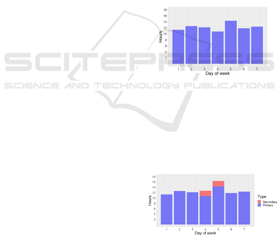
As an example, consider a scenario where a sailor

is serving aboard a ship at sea and is working roughly

12 hours per day. The total workload of the sailor

before any secondary duty hours are scheduled is

shown in Figure 1 where Day 1 corresponds to Monday.

Figure 1: Plot of one week of total workload before

secondary duty hours are added.

The sailor is assigned a secondary duty. On

Thursday morning, the sailor becomes aware that

they have two days to complete four hours of work

for their secondary duty. This means that four hours

of secondary duty work have to be assigned to

Thursday and Friday, which correspond to the two-

day window of this instance. If the time is divided

equally between the two days, they end up working

16.3 hours on the Friday and only 12.7 hours on the

Thursday, as shown in Figure 2.

Figure 2: Plot of one week of total workload when the

secondary duty hours are evenly distributed. Two hours are

added to both Thursday and Friday in red.

WAPAT 2023 - Special Session on Workforce Analytics - Practical Application and Theory

264

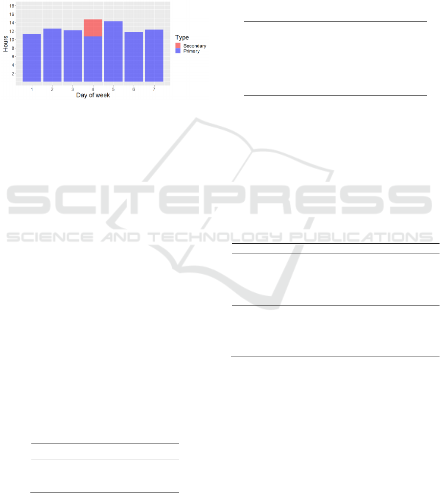
If the sailor knew that they were going to be

working more hours on Friday than Thursday, they

may choose to complete all four hours of the

secondary duty on Thursday. The heuristic approach

has the same effect, since the four required hours are

divided into two units of two hours each, both of

which are assigned to Thursday. This leads to a total

workload of 14.7 hours on Thursday and 14.3 hours

on Friday, as is seen in Figure 3.

Figure 3: Plot of one week of total workload when the

heuristic approach is used to allocate the secondary duty

hours. All four hours are added to Thursday in red.

Through use of the heuristic approach to allocate

hours, the maximum workload encountered on a

single day is reduced from 16.3 to 14.7. More

importantly, the heuristic approach follows how

individuals manage time, making the model more

representative of reality.

4 NOTIONAL EXAMPLE OF

RESULTS

An example of the application of the simulation

model is presented in this section. Notional data is

used.

Consider a sailor serving aboard a ship that will

spend the first half of a year at sea in an operational

footing before returning to home port for the

remainder of the year. The unit state inputs for this

case are shown in Table 3, where an additional month

has been added to the beginning and end to avoid edge

effects, as discussed in Section 3.3. It is the year

spanning from the 2nd to 13th months that is output

for analysis.

Table 3: Unit state for each month in the notional example.

Months Unit state

1-7 At sea on operation (SO)

8-14 Alongside home port (AH)

The sailor’s primary duties require between 10

and 15 hours per day when at sea on operation, with

a most-likely value of 12.5. When in home port, their

primary duty time requirements are shorter and less

varied and range from seven to nine hours per day

with a value of eight being the most likely. This is

summarized in Table 4, which shows only the

relevant data from the primary duty input file.

Table 4: The primary duty input values for the sailor being

described in the notional example.

SO: Minimum required hours per day 10

SO: Most-likely required hours per day 12.5

SO: Maximum required hours per day 15

AH: Minimum required hours per day 7

AH: Most-likely required hours per day 8

AH: Maximum required hours per day 9

On top of their primary duties, the sailor is also

responsible for two secondary duties. They do not

share the duties with any other sailors, so they are

responsible for the full time requirements of both. The

first duty requires just as much work when the ship is

at sea on operation as when it is alongside its home

port, but the other is much more demanding when the

ship is at sea. The relevant data from the secondary

duty input file are shown in Table 5.

Table 5: The input values for the two secondary duties

assigned to the sailor in the notional example.

Duty 1 2

SO: Instances per year 26 8

SO: Minimum required hours of instance 2 10

SO: Most-likely required hours of instance 4 15

SO: Maximum required hours of instance 6 20

SO: Days in window 2 5

AH: Instances per year 26 2

AH: Minimum required hours of instance 2 3

AH: Most-likely required hours of instance 4 6

AH: Maximum required hours of instance 6 9

AH: Days in window 2 2

Based on the input values, and without running

the simulation, the sailor is expected to spend 12.5

hours on their primary duties each day when at sea on

operation. Over the course of the six months spent on

operation, they would expect to spend 52 hours on

their first secondary duty and 60 hours on their second.

With no further knowledge of the secondary duties,

one could assume that they can be divided up over all

180 days of the time period and result in a daily

workload of approximately 37 minutes per day. This

would bring the length of the overall sailor’s workday

from 12.5 hours to roughly 13.1 hours, leaving 10.9

Quantifying the Impact of Secondary Duties on Sailor Workload Through Simulation

265

hours for rest and recovery. It is unlikely that such a

case would be flagged as unreasonable or as putting

the sailor at high risk of becoming fatigued.

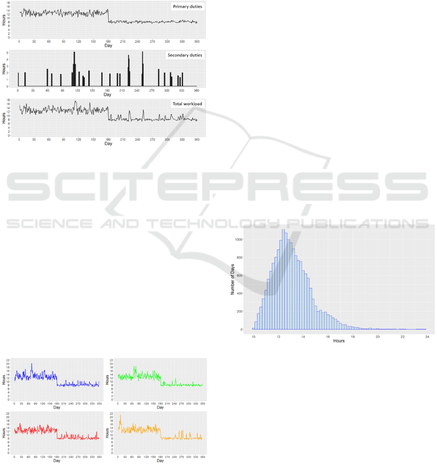
When the simulation model is run using the inputs,

the impact of the secondary duties on individual days

becomes clear. An example of a single simulated year

(a single replication) is shown in Figure 4, where it is

seen that the sailor works many more hours during

some days than others regardless of the state of the

ship.

Figure 4: Primary duty, secondary duty, and total workload

of a single simulated year for the sailor in the notional

example.

Looking specifically at the first six months of this

replication, corresponding to when the sailor is at sea

on operation, the sailor works between 10.39 and

17.52 hours each day with a mean of 12.89 hours. The

sailor is assigned secondary duty work hours on 26 of

the 180 days.

The stochastic nature of the model makes it

necessary to analyze multiple replications to ensure

accurate statistics are generated, since consecutive

replications will differ. For example, the next four

replications of the notional experiment are plotted in

Figure 5. The minimum number of hours worked in

each replication are 10.23, 10.07, 10.25, and 10.31,

respectively. The corresponding maximum values are

Figure 5: Four additional replications of a simulated year

for the sailor in the notional example.

20.17, 18.65, 16.64, and 21.12. Far more variation is

seen in the maximum total workload values than the

minimum values due to the difference in sample size

of days with low and high workload. This is due to

small total workload values occurring when no

secondary duties are performed, which is relatively

common, and high total workload values occurring

when multiple instances of secondary duties being

performed overlap, which is less common.

In total, 100 replications of the notional example

simulation were completed and aggregate statistics

were generated from those. Focusing on the first six

months of the simulated year, when the ship is at sea,

a total of 18,000 simulated days are contained in the

100 replications. The mean of all the simulated days

is 13.10 hours, which agrees with the calculation

performed without using the model. The shortest

workday seen is 10.04 hours and the longest is 23.71

hours. The maximum value represents a day where

many secondary duty instances are occurring

concurrently. While an outlier, the existence of such

a day demonstrates the risk associated with assigning

multiple secondary duties to a single sailor.

The total workloads of all 18,000 days are

represented in the distribution shown in Figure 6. It is

seen that the triangular distribution of the primary

duty workload, which ranges from a minimum of 10

to a maximum of 15, is the dominant feature of the

distribution, although the addition of secondary duty

hours adds significant positive skew.

Figure 6: The distribution of total workload in the 18,000

simulated days falling within the first six months of the

notional example.

In Table 6, the probability of workloads

exceeding certain thresholds are given. This

probabilistic treatment provides a much better sense

of the workload the sailor would experience during

the time at sea than the mean value of 13.1 hours

computed before completing the simulation. For

example, more than five percent of days require the

sailor to work at least 16 hours, leaving less than eight

WAPAT 2023 - Special Session on Workforce Analytics - Practical Application and Theory

266

hours for rest and recovery. Such a statistic is more

suitable for predicting fatigue than the daily mean.

Table 6: Probability of daily workloads more than various

numbers of hours computed for the first six months of the

notional example.

Number of hours

worked

Probability of day requiring

more work

10 1

11 0.9415

12 0.7530

13 0.4679

14 0.2426

15 0.1082

16 0.0524

17 0.0197

18 0.0078

19 0.0034

20 0.0014

21 0.0008

22 0.0003

23 0.0002

24 0

5 VERIFICATION

The model was first implemented in the R

programming language version 4.1.1 (R Core Team,

2021). Verification of the R version was first

completed by comparing statistics generated using

simulated schedules to those computed analytically.

Next, several experiments were designed to isolate

and challenge code features so that errors in the

implementation could be identified and corrected.

The simulation model was then implemented a

second time in Python version 3.8.8 (Python Software

Foundation, 2021). The Python implementation made

use of the Pandas package (Pandas Development

Team, 2021) to allow it to closely follow the R

implementation. Identical experiments could then be

run in both implementations and the results could be

compared to check for issues with either

implementation or the functionality of the packages

involved.

As an example, the experiment discussed in the

notional example was run in both Python and R.

Table 7 summarizes results from both implemen-

tations. Values from the first six months are shown to

avoid conflating time at sea with time in port. The

results of single replications differ in R and Python,

but this is expected due to the stochastic nature of the

model. Similar differences were seen when

comparing individual replications performed in the

same programming language. The results converge

when many replications are considered, as is done in

the table. It is also noted that values that include

secondary duties tend to display more variation in the

mean between replications, which manifests as a

larger standard error. This is due to the limited

number of secondary duty instances in a year,

meaning the sample size of days with secondary duty

hours is smaller than that for days with primary duty

hours.

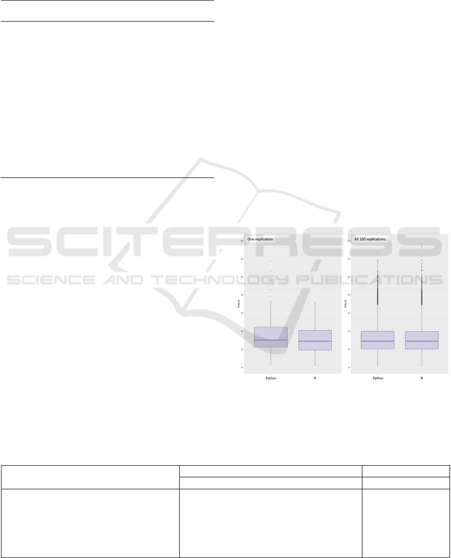
The distributions of daily total workload hours

simulated for the sailor from the notional example in

one replication and 100 replications are compared in

Figure 7. Again, only the first six months are included.

When considering all 100 replications, only the

outliers are discernibly different when comparing the

Python and R outputs.

Figure 7: Distributions of total workload hours computed in

both Python and R.

Table 7: Summary of results for an experiment performed in both R and Python. 100 replications were completed.

Output variable Mean Standard Error

Python R |∆| Python R

Mean daily primary duty workload (hours) 12.49865 12.50428 0.00563 0.00676 0.00748

Mean daily secondary duty workload (hours) 0.61707 0.59184 0.02523 0.01640 0.02001

Mean daily total workload (hours) 13.11571 13.09612 0.01959 0.01752 0.02125

Minimum daily total workload (hours) 10.25510 10.26931 0.01421 0.01256 0.01384

Maximum daily total workload (hours) 18.93740 18.58606 0.35134 0.17311 0.16486

Days with > 16 hours of total workload (days) 9.68 9.43 0.25 0.44 0.53

Quantifying the Impact of Secondary Duties on Sailor Workload Through Simulation

267

6 PERFORMANCE

Performance benchmarking was completed using an

experiment designed to imitate simulating a large

crew: 100 replications of schedule simulation for a

crew consisting of more than 200 positions that is

assigned 58 secondary duties. Primary duty workload

inputs were identical for most unit positions, with a

few excursions inserted manually. Similarly, the

inputs of only a few secondary duties were unique.

The assignment of secondary duties to unit positions

was mostly ordinal: the Nth secondary duty was

assigned to the unit position occupying the Nth

position in the list. A few exceptions were inserted

manually so shared secondary duties and cases of

sailors being assigned multiple secondary duties

would exist in the test data.

Testing was done on a laptop with a four-core 1.9

GHz processor. The results are presented in Table 8,

where it is seen that the Python version executes

roughly 12 times faster than the R version despite

being structured similarly through the use of the

Pandas package and data frames.

Table 8: Benchmarking of the R and Python versions.

Run time

(minutes:seconds)

6:01

Python

0:34

7 CONCLUSION

A model that simulates sailor workload has been

presented. By combining primary and secondary

duties stochastically, it is seen that schedules

produced by the model provide a fuller description of

sailor working life than deterministic estimates of

expected workday lengths. The simulated schedules

are ideal for use in applications where extreme values

in daily workload must be considered including crew

design and research into crew fatigue.

Monte Carlo experimentation using the model can

be used to identify individual secondary duties or

combinations of secondary duties that have a large

impact on sailor workload. In this way, the model can

be used to guide the assignment of secondary duties

or identify secondary duties that may need to be

adjusted or shared between multiple sailors.

ACKNOWLEDGEMENTS

The author would like to thank Cdr Karine

L’Archevêque, LCdr Aislinn Joiner, CPO2 Rayon

Murdock, CPO1 Nathalie Scalabrini, and CPO1

Phillip Gormley for acting as patient and attentive

subject matter experts.

REFERENCES

Chief of Naval Operations (2021). Naval total force

manpower policies and procedures. OPNAVINST

100.16L CH-3. Department of the Navy, Washington,

DC.

Chow, R., Lamb, M., Charest, G., Labbé, D. (2016).

Evaluation of current and future crew sizes and

compositions: Two RCN case studies. Naval Engineers

Journal, 128(4), 59-64.

Clark, C., E. (1962). Letter to the editor—The PERT model

for the distribution of an activity time. Operations

Research, 10(3), 405-406. https://doi.org/10.1287/opre.

10.3.405.

Cordle, J., P. (2019). Manning matters. U.S. Naval Institute

Blog (December 20). https://blog.usni.org/posts/

2019/12/20/manning-matters.

Garbacz, B., D. (2019). How increased manning affects

crewmember’s workload inport and underway: Results

of a study onboard two U.S. Navy destroyers in basic

phase. Naval Postgraduate School, Monterey, CA.

Hollins, R., Leszczynski, K., M. (2014). USN manpower

determination decision making: A case study using

IMPRINT Pro to validate the LCS core crew manning

solution. Naval Postgraduate School, Monterey, CA.

Pandas Development Team (2021). pandas-dev/pandas:

Pandas 1.2.4 (v1.2.4). Zenodo. https://doi.org/10.5281/

zenodo.4681666

Python Software Foundation (2021). The Python language

reference (3.8.13). https://docs.python.org/3.8/referen

ce/index.html#reference-index.

R Core Team (2021). R: A language and environment for

statistical computing. R Foundation for Statistical

Computing, Vienna, Austria.

WAPAT 2023 - Special Session on Workforce Analytics - Practical Application and Theory

268