Human Motion Prediction on the IKEA-ASM Dataset

Mattias Billast

1 a

, Kevin Mets

2 b

, Tom De Schepper

1 c

, Jos

e Oramas

1 d

and Steven Latr

1 e

University of Antwerp - imec, IDLab, Department of Computer Science, Sint-Pietersvliet 7, 2000 Antwerp, Belgium

University of Antwerp - imec, IDLab, Faculty of Applied Engineering, Sint-Pietersvliet 7, 2000 Antwerp, Belgium

Keywords:

Motion Prediction, Graph Neural Network, IKEA-ASM.

Abstract:

Motion prediction of the human pose estimates future poses based on the preceding poses. It is a stepping

stone toward industrial applications, like human-robot interactions and ergonomy indicators. The goal is to

minimize the error in predicted joint positions on the IKEA-ASM dataset which resembles assembly use cases

with a high diversity of execution and background of the same action class. In this paper, we use the STS-

GCN model to tackle 2D motion prediction and make various alterations to improve the performance of the

model. First, we pre-processed the training dataset through ﬁltering to remove outliers and inconsistencies

to boost performance by 31%. Secondly, we added object gaze information to give more context to the body

motion of the subject, which lowers the error (MPJPE) to 10.1618 compared to 18.3462 without object gaze

information. The increased performance indicates that there is a correlation between the object gaze and body

motion. Lastly, the over-smoothing of the Graph Convolutional Network embeddings is decreased by limiting

the number of layers, providing richer joint embeddings.

1 INTRODUCTION

Motion prediction of the human pose estimates future

poses based on the preceding poses. Prediction in the

spatial and temporal dimensions is a challenging task

that has multiple purposes. The overall goal is to im-

prove human-robot interactions, determine ergonomy

indicators and increase safety. A possible use case is

that users get an alert in a VR/AR setup when they are

getting too close to a safety zone or when their pos-

ture is not ergonomic for long assembly tasks. The

human pose is represented by a graph connecting 17

body joints. Typically, the time and space domains

are modeled separately in human pose motion predic-

tion. The time domain can be modeled with Recurrent

Neural Networks (RNN), Long Short-Term Memory

networks (LSTM), Gated Recurrent Unit (GRU), and

recently with Transformers. The joint coordinates and

their interactions are rather modeled with Graph Con-

volutional Networks (GCN). We opted for the STS-

GCN model (Soﬁanos et al., 2021) as it models the

space and time dimensions together as both dimen-

https://orcid.org/0000-0002-1080-6847

https://orcid.org/0000-0002-4812-4841

https://orcid.org/0000-0002-2969-3133

https://orcid.org/0000-0002-8607-5067

https://orcid.org/0000-0003-0351-1714

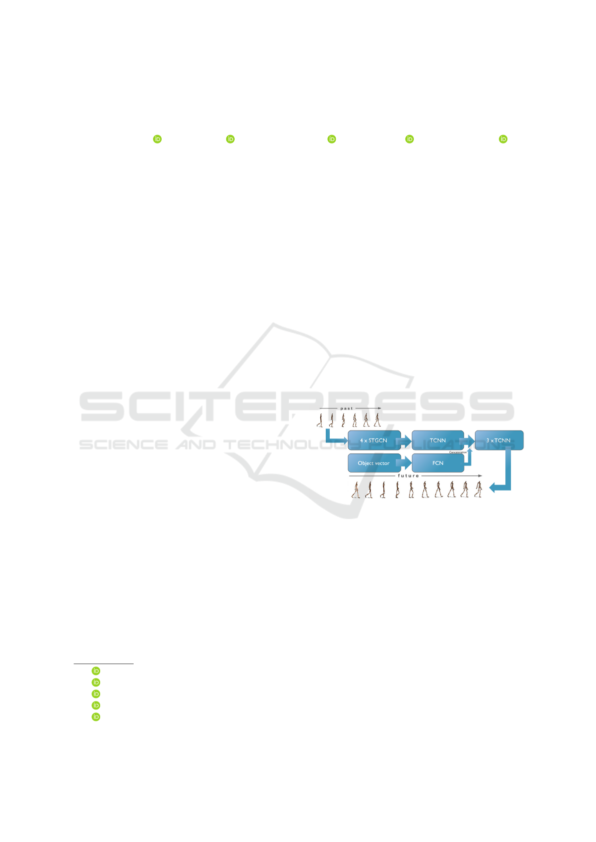
Figure 1: The STS-GCN-2D model architecture with added

object information.

sions are correlated while limiting cross-talk between

the two. Both factors limit the number of parameters

of the model, which enables fast real-time applica-

tions and the scalability of the model. The STS-GCN

model is meant for 3D pose motion prediction but we

repurposed it for 2D human pose motion prediction

on the IKEA-ASM dataset (Ben-Shabat et al., 2020)

for the ﬁrst time. The goal is to upscale again in fu-

ture work but the 2D case is a good subject to analyze

alterations we made to the original dataset and model.

2D pose estimation models on RGB videos (He et al.,

2017) are also more accurate than their 3D pose coun-

terparts, as the depth dimension is difﬁcult to estimate

with only an RGB camera. All the models are trained

on 2D pose estimations without manual annotations.

Our contributions are three-fold: ﬁrst, we smooth the

906

Billast, M., Mets, K., De Schepper, T., Oramas, J. and Latré, S.

Human Motion Prediction on the IKEA-ASM Dataset.

DOI: 10.5220/0011902300003417

In Proceedings of the 18th International Joint Conference on Computer Vision, Imaging and Computer Graphics Theory and Applications (VISIGRAPP 2023) - Volume 5: VISAPP, pages

906-914

ISBN: 978-989-758-634-7; ISSN: 2184-4321

 2023 by SCITEPRESS – Science and Technology Publications, Lda. Under CC license (CC BY-NC-ND 4.0)

training dataset with simple ﬁltering methods, to re-

move jumps and noise in the joint coordinates. Sec-

ondly, we add gaze context of the subject by includ-

ing the object they are looking at or interacting with

(shown in Figure 1 as object vector). Adding infor-

mation about which object the subject is looking at,

is also relevant in VR/AR use cases where there is

egocentric data that can be added to the model and

there is already work showing correlations between

the active object and motion prediction (Zheng et al.,

2022). Thirdly, we alter the number of GCN layers

to minimize the over-smoothing effect on representa-

tions (Chen et al., 2020). Over-smoothing in a GCN

occurs when there are too many layers and the nodes

become indistinguishable from each other. This hap-

pens because, at each layer, a node is updated with an

aggregate of neighboring nodes’ feature vectors.

2 RELATED WORK

All recent human pose motion prediction uses deep

learning models to leverage the motion patterns in the

data.

Temporal Encoding. (Butepage et al., 2017) use

Fully Connected Layers to temporally encode the in-

puts and decode them to look like the future outputs.

Another temporal representation technique is RNN

(Zhang et al., 2020) LSTM (Hu et al., 2019; Chiu

et al., 2019), GRU (Yuan and Kitani, 2020; Adeli

et al., 2020). These RNN models perform well but

are difﬁcult to train due to the vanishing/exploding

gradient problem, and have millions of parameters

(Gopalakrishnan et al., 2019) which require more data

to train appropriately. The amount of parameters is

also related to the number of computations, training

time, and inference speed. Similar to an RNN, mod-

eling the time domain with Transformers (Mart

ınez-

Gonz

alez et al., 2021; Vendrow et al., 2022) reports

good results but also requires a lot of data. We opted

for the Temporal Convolutional Layers (TCN) (Luo

et al., 2018) as it is the state of the art with a relatively

low amount of parameters.

Spatial Encoding. Regarding the spatial aspect,

a Graph Convolutional Network (GCN) (Mohamed

et al., 2021; Soﬁanos et al., 2021; Li et al., 2021; Liu

et al., 2021) can represent the spatial interactions be-

tween joints in a natural way. The adjacency matrices

can be handcrafted in the shape(Li et al., 2021) of the

human pose or they can be trained iteratively by al-

lowing connections between all nodes(Soﬁanos et al.,

2021).

IKEA-ASM. To the best of our knowledge, mo-

tion prediction on the IKEA-ASM (Ben-Shabat et al.,

2020) dataset has not been done. Most of the work

on this dataset considers action recognition (Zhao

et al., 2022), action segmentation (Ghoddoosian et al.,

2022), and video alignment (Haresh et al., 2021;

Kwon et al., 2022). The most recent work on this

dataset (Diller et al., 2022) tackles action recognition

and shows that characteristic poses of actions and the

action labels are strongly correlated, which supports

the use of context information when predicting poses.

3 METHODOLOGY

3.1 Problem Formulation

Motion prediction estimates the 2D coordinates of V

joints for K frames given the previous T frames with

V joints’ coordinates as input. The goal is to min-

imize the Mean Per Joint Positional Error (MPJPE)

of the estimated joint coordinates and their ground

truths. The following equation gives the MPJPE:

MPJPE =

V K

∑

k=1

∑

v=1

k ˆx

− x

(1)

where ˆx

and x

are respectively the predicted coor-

dinates and the ground truth coordinates of joint v at

time k.

3.2 STS-GCN

For all the experiments, the STS-GCN model (Soﬁ-

anos et al., 2021) is used. It consists of Spatio-

Temporal Graph Convolutional layers (STGCN) fol-

lowed by Temporal convolutional layers (TCNN), see

Figure 1. The STGCN layers allow full space-space

and time-time connectivity but limit space-time con-

nectivity by replacing a full adjacency matrix with the

multiplication of space and time adjacency matrices.

The obtained feature embedding of the graph layers is

decoded by four TCN layers which produce the fore-

casted human pose trajectories.

The motion trajectories in a typical GCN model are

encoded into a graph structure with VT nodes for

all body joints at each observed frame in time. The

edges of the graph are deﬁned by the adjacency ma-

trix A

∈ R

V T ×V T

in the spatial and temporal dimen-

sions. The information is propagated through the net-

work with the following equation:

(l+1)

= σ(A

st−(l)

(l)

) (2)

where H

(l)

∈ R

(l)

×V ×T

is the input to GCN layer l

with C

(l)

the size of the hidden dimension which is

Human Motion Prediction on the IKEA-ASM Dataset

907

2 for the ﬁrst layer, W

(l)

∈ R

(l)

×C

(l+1)

are the train-

able graph convolutional weights of layer l, σ the ac-

tivation function and A

st−(l)

is the adjacency matrix at

layer l.

The STS-GCN model alters the GCN model by re-

placing the adjacency matrix with the multiplication

of T distinct spatial and V distinct temporal adjacency

matrices.

(l+1)

= σ(A

s−(l)

t−(l)

(l)

) (3)

where A

s−(l)

∈ R

V ×V

describes the joint-joint rela-

tions for each of T timesteps and A

t−(l)

∈ R

T ×T

de-

scribes the time-time relations for each of V joints.

This version limits the space-time connections and

reports good performance (Soﬁanos et al., 2021). It

lowers the number of parameters needed which is an

advantage for real-time applications as it decreases

inference speed. The trainable adjacency matrices

with full joint-joint and time-time connections have

attention properties as some nodes/timeframes will be

more important for the predicted motion. Signed and

directed graphs contain richer information to repre-

sent a larger variation of embeddings. In other words,

the adjacency matrix can be asymmetrical with pos-

itive and negative weights. These negative weights

have opposite semantic meaning, so a node can be af-

fected by another node in two opposite ways which

create greater variation.

3.3 Object Information

The idea to use gaze information is explored in Zheng

et al. (Zheng et al., 2022) and shows great poten-

tial. We can hypothesize that the objects the subject

is looking at and interacting with, are correlated with

the motion trajectories. We add the context informa-

tion into the model by concatenating an encoded ob-

ject vector v

of the object that the subject is cur-

rently looking at with the feature embeddings after

one TCNN layer. The concatenation of object vec-

tor and TCNN feature embeddings is shown in Fig-

ure 1. The added input information is ”oracle” data

as we have the annotated action descriptions, which

contain the objects the subject is interacting with. All

(T+K) frames are sampled from the same action in all

experiments to have one action description per sam-

ple. The object vector v

∈ R

d×a

is unique depending

on the objects in the action class description of the

sample, with d the maximum number of active ob-

jects together in the scene and a the number of possi-

ble objects in the scene. The ﬁrst dimension is 2 be-

cause there are a maximum of 2 objects in the action

description and the second dimension is 12 as there

are 12 distinct objects in the action descriptions. An

example of multiple active objects is the description

”align leg screw with table thread” which alludes that

the subject interacts with the leg and the table. The

object vector is fed through a fully connected neu-

ral network layer (FCN) with Relu activation function

and K ×V output nodes. The output is then reshaped

to v

∈ R

K×2×V

to be concatenated with the GCN

embeddings. The weights of the FCN are trained to-

gether with the STS-GCN model and adapted based

on the MPJPE loss function. Figure 1 shows a simpli-

ﬁed version of the architecture.

3.4 Oversmoothing in 2D Case

The original STS-GCN model has 4 layers in the

3D case but we hypothesize that this over-smoothens

the features of the graph network in the 2D case.

The features are a weighted average of the neighbor-

ing nodes’ features and in the 2D case, there is less

information to discriminate between nodes. Over-

smoothing in a GCN occurs when the maximum num-

ber of hops between two nodes on the graph is small.

If this number is smaller than the number of layers,

all nodes contain information about other nodes. At

each layer, the joint is updated with an aggregate of

neighboring joints’ features. The over-smoothing can

be measured with the Mean Average Distance metric

(MAD) (Chen et al., 2020), which is the average co-

sine distance between the hidden representations of

node pairs. By lowering the number of layers, the

MAD value increases and the over-smoothing effect

reduces.

3.5 Using Fewer Joints

The joints that are not occluded generate better pose

estimates compared to occluded joints. The lower

body joints are occluded behind a table in 50% of

the videos (Ben-Shabat et al., 2020). We analyze the

cases where only 2 (hands) and 13 (upper body) joints

are used, to remove noisy data from the data. Figure

2 shows the different graph structures that are used as

input, the kinematic tree with 2 joints (hands) is not

visualized as it is just 2 nodes. The hands’ case is also

a ﬁrst step towards VR/AR use cases with an egocen-

tric view when the only visible joints are the hands.

4 IMPLEMENTATION DETAILS

All models use 4 TCN layers, but we vary between

2 and 4 STGCN layers. During training, a range of

learning rates was tested and the range of 2 × 10

−3

−

8 × 10

−3

gave the best results. The batch size is 256

VISAPP 2023 - 18th International Conference on Computer Vision Theory and Applications

908

(a)

(b)

Figure 2: Kinematic tree with (a) 17 and (b) 13 body joints.

for all experiments. To update the weights, an Adam

optimizer is used with β

= 0.9, β

= −.999, and

weight decay parameter λ = 1 × 10

−5

. The numbers

of channels for the STGCN layers are respectively 3,

64, 32, and 64, and the number of channels for all four

TCN layers is 25, equal to the output time frame. All

models are trained for 50 epochs with a learning step

scheduler which lowers the learning rate by a factor

γ = 0.1 at epochs 15, 25, 35, and 40.

5 DATA

The dataset we used is the IKEA-ASM dataset which

consists of 371 assembly videos with 48 unique sub-

jects performing 33 action classes. There are in total

around 3 million frames. Figure 5 shows the num-

ber of samples per action class in a logarithmic scale.

The samples’ distribution has a large inﬂuence on the

results and generated outputs of the models. For ex-

ample, the action ”spin leg” is a predominant action in

the dataset but only requires little motion to complete

the action, i.e. turning of the wrist. Thus, models

with a more static forecast are dominant. We chose

the IKEA-ASM dataset because it is directly related

to assembly use cases of motion prediction and has a

high diversity of the same action class as the same fur-

niture is assembled in a variety of ways with different

backgrounds.

5.1 Data Filtering

All frames are annotated by a keypoint-rcnn model

(He et al., 2017). This works most of the time, as can

be seen in a qualitative example in Figure 4, but there

are still jumps in the data when joints are occluded.

Figure 3a shows some examples of the jumps in co-

ordinates in the data for a single joint. To alleviate

(a)

(b)

Figure 3: Data sample example: (a) the right wrist coordi-

nates as a time series with various ﬁlters and (b) a snapshot

at the frame when the jump in the time series occurs as the

right wrist is occluded.

Figure 4: Qualitative example of human pose estimator to

annotate data.

the problem of the high-frequency noisy data, multi-

ple smoothing pre-processing methods are tested, i.e.

a median ﬁlter (Justusson, 1981), and a discrete Fast

Fourier Transform (DFT) lowpass ﬁlter (Nussbaumer,

1981). The DFT ﬁlter transforms the coordinate of

the time series to the discrete frequency domain and

only the ﬁrst 100 frequencies (DFT 100) are used to

Human Motion Prediction on the IKEA-ASM Dataset

909

Figure 5: Distribution of actions in the IKEA-ASM dataset.

reconstruct the time series, thus removing the high-

frequency oscillations. The median ﬁlter slides a win-

dow of size x over the time series and returns the

median value within that window. Window sizes 21

(Median 21) and 41 (Median 41) are considered in

the experiments. Figure 3a shows an example of each

smoothing method and Figure 3b shows a frame when

a jump in the right wrist coordinates’ time series oc-

curs.

6 RESULTS

In Tables 1, 2, 3, and 4, the MPJPE is listed for the

various experiments. All experiments are done with

10 input frames and 25 predicted frames correspond-

ing with a 1000ms prediction horizon. This setup is

also used in most motion prediction benchmarks, al-

lowing easy comparison with other methods. The re-

sults with the various modiﬁcations, i.e. data smooth-

ing, adding object context, only using a part of the

kinematic tree, and limiting the amount of STGCN

layers are reported.

6.1 Baseline Results

To start, we implemented simple baseline predictions

to have an indication of the relative performance. A

ﬁrst baseline is a static pose prediction where the last

observed pose is the predicted pose throughout the

prediction horizon. As many static actions exist in the

dataset, the ﬁxed position baseline works relatively

well, as shown in Table 1. Other simple baselines like

predicting the position of joints based on the average

velocity, acceleration, and direction of the joints in the

last 10 observed frames do not improve on the result

of the ﬁxed position baseline on the original dataset.

This is mainly due to the outliers and inconsisten-

cies in the data without pre-processing. These incon-

sistencies are mainly due to the differences in body

joints’ estimation of subsequent frames. The predic-

tion based on the average velocity and acceleration is

given by the following equation:

= P

input

+ k

× v

input

× i +

× a

input

× i

(4)

where P

is the predicted pose at frame i, ranging from

1 to 25, P

input

is the last pose of the input, k

and k

are

the damping parameters, v

input

is the average velocity

of the input, and a

input

is the average acceleration of

the input.

6.2 Pre-Processing

We tested three different pre-processing ﬁlters, i.e.

DFT 100, Median 21, and Median 41. The DFT 100

ﬁlter did smooth away outliers but introduced a si-

nusoidal wave pattern when the original joint coor-

dinates remained constant. Other frequency cutoffs

were considered but they either smoothed too much

or too little. The median ﬁlter with a window of 41

(Median 41) smoothed away too much of the origi-

nal data, while the median ﬁlter with a window of 21

(Median 21) performed best as it ﬁltered outliers but

still remained true to the original data when there is

little noise.

6.2.1 Baselines

The baseline prediction, where a ﬁxed velocity of the

body joints is considered instead of a ﬁxed position

based on the input frames works better when validated

on the smoothed dataset. Also including the average

joints’ acceleration in the observed frames, see Equa-

tion 4, improves the prediction even further on the

smoothed dataset. An important note is that the aver-

age velocity and acceleration are damped with a factor

and k

of 0.2 and 0.05 respectively as the predic-

tions otherwise overshoot the actual movements for a

horizon of 1000ms.

6.2.2 STS-GCN

In Table 1 the three data ﬁlters are examined together

with the STS-GCN-2D model, i.e. DFT 100, Median

21, and Median 41. As shown in Table 1 the Me-

dian 41 ﬁlter worked best when the validation data

was also smoothed but this could mean that the data is

over-smoothed which is easier for a model to predict

and does not give a fair comparison. Hence, all the

validation data in subsequent experiments is the orig-

inal un-processed data. When testing on the original

data, using the Median 21 ﬁlter for training general-

izes slightly better, so this ﬁlter is used for the next

experiments. The sinusoidal wave the DFT 100 ﬁlter

introduces, results in a jerky and periodic motion pre-

diction of the joints and thus poor testing performance

on the original data.

VISAPP 2023 - 18th International Conference on Computer Vision Theory and Applications

910

Table 1: MPJPE results of the baselines and adding various dataset smoothing methods.

Model Nodes #STGCN L Object Data train ﬁlter Data val ﬁlter MPJPE

Fixed position 17 - 7 - Original 13.94

Fixed position 17 - 7 - Median 21 11.37

Fixed velocity 17 - 7 - Median 21 10.02

Fixed acceleration 17 - 7 - Median 21 9.7624

STS-GCN-2D 17 4 7 Median 41 Median 41 8.1938

STS-GCN-2D 17 4 7 Median 21 Median 21 9.9145

STS-GCN-2D 17 4 7 DFT 100 DFT 100 9.7385

STS-GCN-2D 17 4 7 Median 41 Original 12.8814

STS-GCN-2D 17 4 7 Median 21 Original 12.6363

STS-GCN-2D 17 4 7 DFT 100 Original 26.5258

STS-GCN-2D 17 4 7 Original Original 18.3462

Table 2: MPJPE results of the isolated improvements on the STS-GCN-2D model.

Model Nodes #STGCN L Object Data train ﬁlter Data val ﬁlter MPJPE

Fixed position 17 - 7 - Original 13.94

STS-GCN-2D 17 4 7 Original Original 18.3462

STS-GCN-2D 17 4 3 Original Original 10.1618

STS-GCN-2D 17 2 7 Original Original 16.7893

STS-GCN-2D 13 4 7 Original Original 11.8570

6.3 Architecture Changes

Table 2 shows the results where various changes are

applied to the STS-GCN-2D model.

6.3.1 Active Object Information

Adding object information does perform better than

the model without object information, conﬁrming the

hypothesis that there is a correlation between the ob-

ject the subject is interacting with and the joints’ mo-

tion trajectories. Adding object context has the best

overall MPJPE as there is a lot of added input infor-

mation that is derived from the manually annotated

action labels. In the future, an oracle can be replaced

by an active object estimator which makes it more re-

alistic.

6.3.2 Skeleton Conﬁguration

Limiting the number of joints to 13 (upper body) to

remove unnecessary or error-prone movement regard-

ing the action task at hand improves the results com-

pared to the model with 17 joints. The upper body

has fewer occlusions than the lower body which is oc-

cluded behind a table for 50% of the videos. Follow-

ing this reasoning, the joints’ coordinates of the upper

body are overall more accurate.

6.3.3 Minimizing Over-Smoothing GCN

Using two STGCN layers instead of four provides a

small improvement for the simple 2D model on all

joints. By only using 2 layers, the MAD value in-

creased from 0.58 to 0.60. This is a marginal gain but

it did translate to a small increase in performance on

the testing data, as we compare row 2 and 4 in Table

2. A minimal increase in MAD value by lowering the

number of layers to two indicates that there is less

over-smoothing of the graph representation than with

four layers.

6.3.4 Combining of Improvments

Table 3 shows the performance achieved by various

combinations of the previously explained changes.

Active Object + Smoothing. The table shows that

combining object context and training on smoothed

dataset does not necessarily improve the results on

the original dataset. A possible explanation might

be that high-frequencies present in the original (non-

smoothed) dataset give an indication of what motion

is going to occur and combining with object context

gives a good prediction.

Custom Skeleton Conﬁguration + Smoothing.

Limiting the number of joints to 13 (upper body) or 2

(hands) to remove unnecessary or error-prone move-

ment regarding the action task at hand has different

results. The case with 13 joints improves the results

Human Motion Prediction on the IKEA-ASM Dataset

911

Table 3: MPJPE results of the combinations of improvements on STS-GCN-2D model, while also including some baselines.

Model Nodes #STGCN L Object Data train ﬁlter Data val ﬁlter MPJPE

Fixed position 17 - 7 - Original 13.94

STS-GCN-2D 17 4 7 Original Original 18.3462

STS-GCN-2D 17 4 3 Original Original 10.1618

STS-GCN-2D 17 4 3 Median 21 Original 12.6789

STS-GCN-2D 13 4 3 Median 21 Original 12.2306

STS-GCN-2D 13 2 3 Median 21 Original 12.8616

STS-GCN-2D 2 4 3 Median 21 Original 16.9668

STS-GCN-2D 2 2 3 Median 21 Original 16.8866

Table 4: MPJPE results of various combinations of STS-GCN-2D model trained on the ﬂoor and table dataset splits.

Nodes #STGCN L Object Data train ﬁlter Data val ﬁlter MPJPE

1 17 4 3 Full split Full split 10.1618

2 17 4 3 Full split Table split 10.1224

3 17 4 3 Full split Floor split 10.1845

4 13 4 3 Full split Full split 11.2891

5 13 4 3 Full split Table split 11.6197

6 13 4 3 Full split Floor split 11.0983

7 17 4 3 Table split Full split 17.5242

8 17 4 3 Floor split Full split 12.6189

9 13 4 3 Table split Full split 15.1431

10 13 4 3 Floor split Full split 12.8331

11 17 4 3 Median21 Table split Full split 15.5269

12 17 4 3 Median21 Floor split Full split 12.9247

13 13 4 3 Median21 Table split Full split 15.2879

14 13 4 3 Median21 Floor split Full split 12.9681

compared to the model with 17 joints. In the hands’

case (2 joints), the results did not improve as there is

too little information on the whole kinematic tree to

make a correct motion prediction of only the hands.

Custom Skeleton Conﬁguration + Smoothing +

2 STGCN Layers. On the other hand, using two

STGCN layers has a factor when only considering

the hands. The reasoning here would be that these

2 joints are over-smoothed as each layer outputs a

weighted average of the neighboring joints. With 4

layers all the information of a speciﬁc node is van-

ished due to this smoothing effect. The MAD value

increased from 0.484 with four layers to 0.729 with

two layers which backs the hypothesis that there is

signiﬁcantly more over-smoothing with four layers.

The hands’ case with improvements still performed

better than the original model with 17 joints and no

improvements, which is a ﬁrst indicator that VR/AR

industrial use cases with motion prediction are fea-

sible. This is a good result as the MPJPE gives a

”per joint” error but when we only evaluate the hands’

joints which are the joints with the most movement in

an assembly task, it is difﬁcult to compare the differ-

ent settings. Following this reasoning, the hands’ case

is the most difﬁcult setting to perform well.

Figures 6 and 7 show qualitative results of the pre-

dicted sequences of different actions by the STS-GCN

model with object context, 2 STGCN layers, and

trained on the smoothed dataset.

6.4 Occlusions

To examine the effect of occlusions, the dataset is split

into two parts, one with a table in front of the subject

and one without a table. Table 4 shows the results

when only using these splits of the dataset, i.e. splits

where there is respectively a table (Table split) or not

(Floor split) in the assembly scene which can occlude

the lower part of the body and increase the noise in

the dataset. The models trained on the full data per-

formed similarly on the original, table, and ﬂoor val-

idation datasets. We can reason that the model is

robust to the occluded data samples. On the other

hand, the models trained on the ﬂoor dataset gener-

alize much better to the full dataset than the mod-

els trained on the table dataset with occlusions. The

largest improvement, when trained on the table split,

is observed when 13 nodes instead of 17 are used and

VISAPP 2023 - 18th International Conference on Computer Vision Theory and Applications

912

(a)

(b)

Figure 6: Separated prediction (purple) and ground truth (green) motion sequences of the action (a) ”spin leg’ and (b) ”attach

drawer side panel” by the STS-GCN-2D model with object context, trained on the smoothed IKEA-ASM dataset.

(a)

(b)

(c)

Figure 7: Prediction (purple) and ground truth (green) motion sequences of the action (a) ”spin leg’, (b) ”attach drawer

side panel”, and (c) ”attach drawer side panel” by the STS-GCN-2D model with object context, trained on the smoothed

IKEA-ASM dataset.

tested on the full dataset, which can be seen by com-

paring rows 7 and 9 in Table 4. Removing lower body

joints from the training samples boosts the data qual-

ity. This improvement is diminished when the train-

ing set is ﬁltered with a Median 21 ﬁlter because then

the occluded lower body joint estimations are more

accurate and actually add information to the model.

With ﬁltering, it is not opportune to remove the lower

body joints as input.

7 CONCLUSION AND FUTURE

WORK

We summarize our work on 2D motion prediction on

the IKEA-ASM dataset by the following modiﬁca-

tions to the dataset and model. Pre-processing the

dataset to remove outliers and inconsistencies boosts

performance. We added object gaze information to

give more context to the body motion of the subject.

Over-smoothing of the GCN embeddings is decreased

by limiting the number of layers. Lastly, only using

the upper body joints improves the results as the lower

body pose estimations are error-prone.

Future work includes adding baselines mentioned in

the related work section to have stronger compar-

isons. The object gaze information is currently added

as an oracle but in certain use cases it is more realis-

tic to predict the active object given the raw video in-

puts, this problem is tackled in one of the MECCANO

dataset challenges (Ragusa et al., 2022). Adding an

active object detector is one of the possible future di-

rections that can be explored. With 3D human poses,

it is also possible to constrain the possible joint trajec-

tories with the physical constraints of the kinematic

Human Motion Prediction on the IKEA-ASM Dataset

913

tree as there are accurate angles and distances be-

tween nodes in 3D.

ACKNOWLEDGEMENTS

This research received funding from the Flemish Gov-

ernment (AI Research Program).

REFERENCES

Adeli, V., Adeli, E., Reid, I., Niebles, J. C., and Rezatoﬁghi,

H. (2020). Socially and contextually aware human

motion and pose forecasting. IEEE Robotics and Au-

tomation Letters, 5(4):6033–6040.

Ben-Shabat, Y., Yu, X., Saleh, F., Campbell, D., Rodriguez-

Opazo, C., Li, H., and Gould, S. (2020). The ikea

asm dataset: Understanding people assembling furni-

ture through actions, objects and pose.

Butepage, J., Black, M. J., Kragic, D., and Kjellstrom, H.

(2017). Deep representation learning for human mo-

tion prediction and classiﬁcation. In Proceedings of

the IEEE conference on computer vision and pattern

recognition, pages 6158–6166.

Chen, D., Lin, Y., Li, W., Li, P., Zhou, J., and Sun, X.

(2020). Measuring and relieving the over-smoothing

problem for graph neural networks from the topolog-

ical view. In Proceedings of the AAAI Conference on

Artiﬁcial Intelligence, volume 34, pages 3438–3445.

Chiu, H.-k., Adeli, E., Wang, B., Huang, D.-A., and

Niebles, J. C. (2019). Action-agnostic human pose

forecasting. In 2019 IEEE Winter Conference on Ap-

plications of Computer Vision (WACV), pages 1423–

1432. IEEE.

Diller, C., Funkhouser, T., and Dai, A. (2022). Forecast-

ing actions and characteristic 3d poses. arXiv preprint

arXiv:2211.14309.

Ghoddoosian, R., Dwivedi, I., Agarwal, N., Choi, C., and

Dariush, B. (2022). Weakly-supervised online action

segmentation in multi-view instructional videos. In

Proceedings of the IEEE/CVF Conference on Com-

puter Vision and Pattern Recognition, pages 13780–

13790.

Gopalakrishnan, A., Mali, A., Kifer, D., Giles, L., and Oror-

bia, A. G. (2019). A neural temporal model for human

motion prediction. In Proceedings of the IEEE/CVF

Conference on Computer Vision and Pattern Recogni-

tion (CVPR).

Haresh, S., Kumar, S., Coskun, H., Syed, S. N., Konin, A.,

Zia, Z., and Tran, Q.-H. (2021). Learning by aligning

videos in time. In Proceedings of the IEEE/CVF Con-

ference on Computer Vision and Pattern Recognition,

pages 5548–5558.

He, K., Gkioxari, G., Dollar, P., and Girshick, R. (2017).

Mask r-cnn. In Proceedings of the IEEE International

Conference on Computer Vision (ICCV).

Hu, J., Fan, Z., Liao, J., and Liu, L. (2019). Predict-

ing long-term skeletal motions by a spatio-temporal

hierarchical recurrent network. arXiv preprint

arXiv:1911.02404.

Justusson, B. (1981). Median ﬁltering: Statistical proper-

ties. Two-Dimensional Digital Signal Prcessing II,

pages 161–196.

Kwon, T., Tekin, B., Tang, S., and Pollefeys, M. (2022).

Context-aware sequence alignment using 4d skeletal

augmentation. In Proceedings of the IEEE/CVF Con-

ference on Computer Vision and Pattern Recognition

(CVPR), pages 8172–8182.

Li, Q., Chalvatzaki, G., Peters, J., and Wang, Y. (2021). Di-

rected acyclic graph neural network for human motion

prediction. In 2021 IEEE International Conference on

Robotics and Automation (ICRA), pages 3197–3204.

IEEE.

Liu, Z., Su, P., Wu, S., Shen, X., Chen, H., Hao, Y., and

Wang, M. (2021). Motion prediction using trajectory

cues. In Proceedings of the IEEE/CVF International

Conference on Computer Vision, pages 13299–13308.

Luo, W., Yang, B., and Urtasun, R. (2018). Fast and furi-

ous: Real time end-to-end 3d detection, tracking and

motion forecasting with a single convolutional net. In

Proceedings of the IEEE conference on Computer Vi-

sion and Pattern Recognition, pages 3569–3577.

Mart

ınez-Gonz

alez, A., Villamizar, M., and Odobez, J.-M.

(2021). Pose transformers (potr): Human motion pre-

diction with non-autoregressive transformers. In Pro-

ceedings of the IEEE/CVF International Conference

on Computer Vision, pages 2276–2284.

Mohamed, A., Chen, H., Wang, Z., and Claudel, C.

(2021). Skeleton-graph: Long-term 3d motion predic-

tion from 2d observations using deep spatio-temporal

graph cnns. arXiv preprint arXiv:2109.10257.

Nussbaumer, H. J. (1981). The fast fourier transform. In

Fast Fourier Transform and Convolution Algorithms,

pages 80–111. Springer.

Ragusa, F., Furnari, A., and Farinella, G. M. (2022). Mec-

cano: A multimodal egocentric dataset for humans be-

havior understanding in the industrial-like domain.

Soﬁanos, T., Sampieri, A., Franco, L., and Galasso, F.

(2021). Space-time-separable graph convolutional

network for pose forecasting. CoRR, abs/2110.04573.

Vendrow, E., Kumar, S., Adeli, E., and Rezatoﬁghi, H.

(2022). Somoformer: Multi-person pose forecasting

with transformers. arXiv preprint arXiv:2208.14023.

Yuan, Y. and Kitani, K. (2020). Dlow: Diversifying latent

ﬂows for diverse human motion prediction. In Euro-

pean Conference on Computer Vision, pages 346–364.

Springer.

Zhang, J., Liu, H., Chang, Q., Wang, L., and Gao, R. X.

(2020). Recurrent neural network for motion trajec-

tory prediction in human-robot collaborative assem-

bly. CIRP annals, 69(1):9–12.

Zhao, Z., Liu, Y., and Ma, L. (2022). Compositional action

recognition with multi-view feature fusion. Plos one,

17(4):e0266259.

Zheng, Y., Yang, Y., Mo, K., Li, J., Yu, T., Liu, Y.,

Liu, C. K., and Guibas, L. J. (2022). Gimo: Gaze-

informed human motion prediction in context. In Eu-

ropean Conference on Computer Vision, pages 676–

694. Springer.

VISAPP 2023 - 18th International Conference on Computer Vision Theory and Applications

914