Analysing Customer Behaviour Using Simulated Transactional Data

Ryan Butler

1 a

and Edwin Simpson

2 b

Department of Engineering Mathematics, University of Bristol, Bristol, U.K.

Intelligent Systems Labs, University of Bristol, Bristol, U.K.

Keywords:

Simulated Transactional Data, Grouped Convolutional Neural Network, Agent-Based Modelling, Know Your

Customer.

Abstract:

This paper explores a novel technique that can aid ﬁrms in ascertaining a customer’s risk proﬁle for the purpose

of safeguarding them from unsuitable ﬁnancial products. This falls under the purview of Know Your Customer

(KYC), and a signiﬁcant amount of regulation binds ﬁrms to this standard, including the Financial Conduct

Authority (FCA) handbook Section 5.2. We introduce a methodology for computing a customer’s risk score

by converting their transactional data into a heatmap image, then extracting complex geometric features that

are indicative of impulsive spending. This heatmap analysis provides an interpretable approach to analysing

spending patterns. The model developed by this study achieved an F1 score of 94.6% when classifying these

features, far outperforming alternative conﬁgurations. Our experiments used a transactional dataset produced

by Lloyds Banking Group, a major UK retail bank, via agent-based modelling (ABM). This data was computer

generated and at no point was real transactional data shared. This study shows that a combination of ABM

and artiﬁcial intelligence techniques can be used to aid ﬁrms in adhering to ﬁnancial regulation.

1 INTRODUCTION

Know Your Customer. The Financial Conduct Au-

thority (FCA) handbook Section 5.2 (Financial Con-

duct Authority, 2004) states that ﬁrms are required to

Know Your Customer (KYC); that is, a customer’s

risk proﬁle should be ascertained before offering a

customer ﬁnancial advice or a ﬁnancial product. KYC

also includes an assessment of a customer’s credit

risk, as well as the anti-money laundering and fraud

checks that a ﬁnancial institution must complete when

a transaction occurs (GOV.UK, 2016). According to

Hyperion (2017), performing KYC checks costs the

average bank £55m annually. In addition, in the UK,

25% of bank applications are abandoned due to KYC

friction, resulting in a further loss of potential rev-

enue. This friction occurs due to extensive reliance

on manual checks, which are both costly for the bank

and cumbersome for the customer. Online checks

have been used in an attempt to solve this issue; how-

ever, these have a high failure rate of up to 20% due

to the poor-quality data that is typically provided by

customers. Lastly, some banks opt to outsource these

checks to onboarding and compliance platforms such

https://orcid.org/0000-0002-8210-1029

https://orcid.org/0000-0002-6447-1552

as Pass Fort (PassFort, 2015), which are costly.

Non-compliance with KYC procedures can also

lead to hefty ﬁnes. In the EU, the “Fifth Anti-

Money Laundering Directive” (5AMLD) penalises

non-compliance with ﬁnes of up to 10% of annual

turnover. For example, Deutsche Bank was ﬁned

£163m for failing to correctly adhere to the preced-

ing legislation (the “Fourth Anti-Money laundering

Directive”, 4AMLD). Similarly, Barclays was ﬁned

£72m for failing to perform 4AMLD checks on sev-

eral ultra-high-net-worth clients. These ﬁnes would

be approximately £2.5bn and £2bn if 5AMLD was ap-

plied retrospectively (Ogonsola and Pannifer, 2017).

Machine Learning (ML) Solutions for KYC. To

comply with KYC legislation and reduce the associ-

ated friction and cost per check, ML techniques have

been proposed to automate KYC processes (Chen,

2020). To address the credit risk assessment as-

pect of KYC, Khandani et al. (2010) applied ML

to transactional data to predict consumer credit de-

fault and delinquency. Their predictions proved to

be highly accurate at forecasting such events in the

3–12-month range. For fraud detection, Sinanc et al.

(2021) used the novel approach of converting credit

card transactions into an image using a Gramian an-

Butler, R. and Simpson, E.

Analysing Customer Behaviour Using Simulated Transactional Data.

DOI: 10.5220/0011902100003393

In Proceedings of the 15th International Conference on Agents and Artiﬁcial Intelligence (ICAART 2023) - Volume 2, pages 499-510

ISBN: 978-989-758-623-1; ISSN: 2184-433X

 2023 by SCITEPRESS – Science and Technology Publications, Lda. Under CC license (CC BY-NC-ND 4.0)

499

gular ﬁelds (GAF) representation before employing a

convolutional neural network (CNN) (LeCun et al.,

1998) to classify whether a transaction was fraud-

ulent. This technique achieved a high F1 score of

85.49%, which exceeds the results of related studies

in the ﬁeld (Sinanc et al., 2021).

However, from a customer safeguarding per-

spective, only Butler et al. (2022) have devel-

oped techniques to ascertain customer risk to deter-

mine whether they should be offered speciﬁc prod-

ucts (FCA Section 5.2 (Financial Conduct Authority,

2004)). This is likely because the majority of avail-

able datasets are designed to train ML models to pre-

dict credit events and fraud (Khandani et al., 2010;

Sinanc et al., 2021) and lack gold labels for customer

spending behaviour. As a result, this work focuses

on the customer safeguarding portion of KYC and at-

tempts to predict the risk of a given customer.

Furthermore, owing to the General Data Protec-

tion Regulation (GDPR) (Wolford, 2016), it is not

possible for ﬁrms to provide researchers with real

transactional datasets for the purpose of developing

ML techniques. Therefore, ABM is typically em-

ployed to produce accurate datasets (Koehler et al.,

2005), but the existing ABM work in this ﬁeld is

concerned with datasets for fraud detection (Koehler

et al., 2005), as opposed to customer safeguarding;

only Butler et al. (2022) has used data produced by

ABM for this aspect of KYC. Thus, utilising ABM to

generate transactional datasets for the purpose of cus-

tomer safeguarding represents a gap in the literature.

In their work on customer safeguarding, Butler et

al. (2022) introduced a novel heatmap representation

of transactional data and used a CNN to classify ge-

ometric features in the heatmap. Theirs is the only

study in the literature to employ a heatmap represen-

tation for time series classiﬁcation (TSC). This repre-

sentation is advantageous compared to conventional

TSC techniques due to its high human interpretabil-

ity. A limitation of this prior work, however, is that

the CNN was only trained to classify basic geomet-

ric features in the heatmaps that are only able to cap-

ture a limited range of behavioural patterns. This

is signiﬁcant from a KYC perspective, as complex

geometric features are indicative of complex spend-

ing behaviours, which can be extracted to inform a

ﬁrm of an individual’s impulsivity, and thus be used

to safeguard a customer. Another limitation is that

a more advanced CNN architecture could have been

used to improve the performance of the geometric fea-

ture classiﬁer, such as a CNN with grouped convolu-

tion (Krizhevsky et al., 2012), a global pooling layer

(Lin et al., 2013), and binary focal cross-entropy loss

(Lin et al., 2017). The methodology could also be

improved by deconstructing the heatmap images into

their geometric components, using contemporary im-

age analysis techniques, which could then be used to

directly infer spending behaviour. Lastly, the eval-

uation could be improved by comparing the perfor-

mance of the heatmap representation with a conven-

tional 1D feature vector that is typically used for TSC.

In this paper, we develop techniques to address

the limitations of previous work using heatmaps for

TSC, and create an algorithm to determine customer

risk using geometric features present in a heatmap.

This results in several per-category risk scores, which

could be used by a ﬁrm to determine whether an indi-

vidual should be offered a speciﬁc ﬁnancial product.

For example, if an individual’s scores show that they

are spending impulsively in the takeaway or restau-

rant categories, it would not be appropriate and con-

trary to FCA section 5.2 (Financial Conduct Author-

ity, 2004) to offer them a cashback card that offers

incentives when eating out.

1.1 Aims and Objectives

The objectives of this study are:

• Using simulated transactional data produced via

agent-based modelling, classify complex geomet-

ric data types present in heatmap representations.

• Show how the heatmap representation is superior

to a conventional feature vector used during TSC.

• Explore whether conventional image analysis

techniques can be used to derive insights about a

customer from the heatmap representation.

• Lastly, develop an algorithm to output a risk

score for a customer that can aid in the customer-

safeguarding aspect of KYC.

2 RELATED LITERATURE

2.1 Contemporary Techniques for TSC

Time series data is composed of “a sequence of

data points indexed in time order” (Bowerman and

O’Connell, 1993). A popular TSC approach in-

volves the use of a nearest neighbour classiﬁer (K-

NN), which is commonly used in conjunction with

the dynamic time warping distance measure as a

baseline classiﬁer for TSC problems (Fawaz et al.,

2019). A large amount of research has been con-

ducted to outperform this baseline such as the devel-

opment of the collective of transformation-based en-

sembles (COTE) (Bagnall et al., 2016), and its succes-

sor HIVE-COTE (Lines et al., 2016). HIVE-COTE

ICAART 2023 - 15th International Conference on Agents and Artiﬁcial Intelligence

500

is considered state-of-the-art (Bagnall et al., 2017),

however it is computationally very expensive and suf-

fers from a lack of interpretability due to it being an

ensemble of multiple classiﬁers.

Image-transform, which converts a time series

into an image before classiﬁcation by a CNN, over-

comes the limitations of HIVE-COTE by both be-

ing highly interpretable and computationally efﬁcient

(Fawaz et al., 2019). An example image transform

technique is the use of recurrence plots (Hatami et al.,

2017). These are a 2D representation of the data’s re-

currences and they have been shown to produce com-

petitive results on the UCR (University of California,

Riverside) time series archive, a collection of datasets

commonly used as a benchmark TSC performance, to

state-of-the-art TSC algorithms (Hatami et al., 2017) .

However, a recurrence plot, while more interpretable

than a raw time series, requires training to derive in-

sights from (Marwan, 2011). To solve this issue,

the heatmap representation has been proposed (But-

ler et al., 2022), which contains pixels whose spatial

positions are directly related to the time dimension,

making it far more interpretable.

2.2 The Heatmap Representation

The heatmap representation is an image-transform

technique for time series data (Butler et al., 2022).

This representation involves using two time dimen-

sions, e.g. day of the week and week number, for

the Cartesian coordinates of a pixel. The value of

the pixel represents an aggregate (e.g. sum) of the

values at that time step; an example heatmap can be

seen in Figure 1. Compared to alternative TSC tech-

niques, the visual representations created by image-

transform are easier for users to interpret. This is be-

cause the spatial position of the pixel is directly re-

lated to the time step of the data, so any geometric

features present can be intuitively understood and be

related back to the context of the data. For example, in

Figure 1, columns of adjacent pixels indicate spend-

ing on consecutive days, while rows of adjacent pixels

indicate spending on the same day of the week. Con-

sequently, this interpretability allows complex tem-

poral relationships, which are challenging for con-

ventional TSC techniques to learn (Wang and Oates,

2015), to be clearly depicted in the image’s geometry.

Lastly, the heatmap technique has rarely been used in

the literature (Butler et al., 2022), and thus represents

a key gap in the literature to be explored.

2.3 Uses of the Heatmap Representation

In Butler et al. (2022), two simulated transactional

datasets were provided to the authors by Lloyds Bank-

ing Group. This data was produced via ABM and

was used to train a CNN classiﬁer, which, in con-

junction with statistical analysis, was able to cate-

gorise accounts based on a heatmap representation.

The heatmap structure used in this paper was a 9×31

image (i.e. 9 months by 31 days) wherein each pixel

represented the normalised sum of the transactions on

a given day. Two types of heatmap geometries were

explored: “line”, where a clear line was present in

the image, and “spotty”, where the pixels were ran-

domly dispersed. The CNN classiﬁer was able to dis-

tinguish between the two data types with an accuracy

of 99.585%. Moreover, statistical analysis was used

to analyse the density and skewness of the heatmap

values. Customers were also labelled based on how

much they spent on a given transaction category as

a proportion of their salary. This was then used to

output a label in each category, which summarised an

individual’s spending behaviour.

However, a limitation of Butler et al. (2022) is

that the CNN classiﬁer was trained on a relatively ba-

sic geometric feature (i.e. the presence of a line in

the heatmap). In this paper we show that this can be

extended by looking at more complex geometric fea-

tures, which indicate more complex customer spend-

ing behaviour. Also, Butler et al. (2022) used a

generic CNN with a single kernel, which means the

CNN can only learn one representation of the input

data, and it is thus limited in the number of features

it can learn. This is disadvantageous as the geometric

features present in a heatmap can be numerous and

highly varied. One solution to this issue explored in

this paper is grouped convolution (Krizhevsky et al.,

2012), which employs two or more parallel CNNs on

the same input image, allowing a greater variety of

features to be learned in parallel (Xie et al., 2016).

Furthermore, the CNN used in Butler et al. (2022)

uses a max pooling layer with a parameter that affects

the pool size. This layer was likely overﬁtted as a side

effect of parameter optimisation (Lin et al., 2013).

Therefore, in this paper we eliminated this parame-

ter by using global pooling (Lin et al., 2013) instead.

In addition, the loss function used in Butler et al.’s

model is sparse categorical cross-entropy, which can

cause a model to yield overconﬁdent predictions and

reduce its ability to generalise to new data (Lin et al.,

2017). As a solution, we implemented binary focal

cross-entropy instead to improve the model’s ability

to generalise (Lin et al., 2017).

Lastly, Butler et al. (2022) analysed the statis-

Analysing Customer Behaviour Using Simulated Transactional Data

501

tics of customer spending independently from the heat

map geometry, before combining the results of both

avenues to reach a ﬁnal spending type classiﬁcation.

This ignores the large number of insights that can

be derived by extracting customer spending statistics

directly from the heatmap itself. Therefore, in this

study, we amalgamate these two approaches by de-

constructing the heatmaps into their constituent ge-

ometry and extracting statistics from these geometric

features. This allows complex spending behaviours

to be analysed as image features and thereby provide

more valuable insights about customer behaviour.

Figure 1: Example 7×40 heatmap i.e., 7 days of the week

by 40 weeks, depicting the sum of an individual’s transac-

tions per day in the time period.

3 METHODOLOGY

3.1 Dataset Simulation

The dataset used in this study was a simulated dataset

provided by Lloyds Banking Group, which was pro-

duced by their in-house, agent-based model (ABM)

(Koehler et al., 2005). The simulation for this dataset

involved 1,304 unique agents within a simulated town

and was processed on a minute by minute timescale

(Butler et al., 2022). An agent was either a vendor or a

customer and the town was modelled as a graph where

each node represented an individual agent and edges

the distance between agents. Traits were randomly

assigned to each agent, based on that agent’s initial

parameters, which affected the probability that they

would carry out a transaction. The initial parameters

for each agent were assigned based on expert knowl-

edge of customer behaviour from the retail banking

community, hence we assume that the overall simula-

tion approximates real world data well (Butler et al.,

2022). Lastly, the dataset produced from this simu-

lation contained information such as the time of the

transaction, the amount, the customer’s balance and

the third party account number/vendor name.

3.2 Overall Algorithm Structure

An outline of the overall algorithm produced by this

study can be seen in Figure 2: it converts customer

transactional data into a series of per-category RGB

heatmaps, which are classiﬁed by a CNN (LeCun

et al., 1998) and analysed using contour detection

(Suzuki and Abe, 1985). The output of both are then

used by the risk score algorithm, which outputs a se-

ries of per-category risk scores for that user.

3.3 Heatmap Design

The transactions to vendors in the dataset were ﬁrst

categorised into 15 groups ranging from “Finances”

to “Pub/Bar” through manual sorting of the vendor

names. The transactions for each customer in a given

category were then converted into three pivot tables,

each of size 7 × 40, where 7 represents the number of

days in a week and 40 the number of weeks present in

the dataset. The ﬁrst pivot table contained a Boolean

array, where 1 represented that there were payments

on a given day and 0 that there were no payments. The

second pivot table contained the sum of the transac-

tions on a given day for that transaction category. The

third pivot table contained the sample standard devi-

ation of payments on a given day. Days where the

number of payments was < 20 were deemed insufﬁ-

cient for yielding a statistically valid sample standard

deviation (Hackshaw, 2008) and were instead set to

0. The second and third pivot tables were then nor-

malised so their values would fall into the 0− 1 range,

enabling these pivot tables to be used as image com-

ponents. The three layers were then combined to pro-

duce a 7 × 40 RGB (Red-Green-Blue) image, with the

R layer composed of the Boolean pivot table, the G

layer the normalised sum pivot table and the B layer

the normalised standard deviation pivot table.

Heatmap Design Justiﬁcation. The Boolean R

layer in the heatmap was chosen because it preserved

the macro-structure of the image so that high-level

features, such as spending on consecutive days and

spending on the same day of the week, were not ob-

scured by variations in the pixel intensity of these fea-

tures. These high-level features could then be eas-

ily identiﬁed, which were found to effectively reveal

an individual’s spending behaviour in a given cate-

gory. The G layer provided information about the

proportion of a customer’s total spending in a cate-

gory on a given day during the 7 × 40 period; this

was found to be signiﬁcant, as sudden variations in

spending during the time period could indicate risky

spending behaviour. Lastly, the B layer provided in-

formation about the nature of an individual’s spend-

ing on a given day, so when it was combined with

the information contained in the G layer, it could in-

dicate whether risky spending behaviour occurred on

that day. For example, if a high proportion of a cus-

tomer’s spending in a category occurred on a speciﬁc

ICAART 2023 - 15th International Conference on Agents and Artiﬁcial Intelligence

502

Figure 2: Overall algorithm produced by this study.

day and there was also a large degree of variability in

their spending on that day, it is possible to infer that

their spending was impulsive.

3.4 Conventional Feature Vector

As a comparison with the heatmap representation, we

also evaluated a conventional 1D time series feature

vector containing a user’s transactions over the 280

day period. These time series were split into the same

categories as the heatmaps to allow for direct com-

parison between the performances of the two feature

vector structures. The 1D time series were produced

in a similar way to the R layer of the heatmap where

there is a 1 on a day’s time step if there was a payment

on that day, and a 0 if there were no payments.

3.5 Labelling Strategy

The customer heatmaps were split into those with a

clear geometric structure in their R layer and those

whose payments were more randomly dispersed over

the period. Heatmaps with clear geometric features

were labelled “Tetris”, owing to the appearance of ge-

ometric features that resembled the components of a

Tetris game (Britannica, The editors of Encyclopedia,

2022). An example Tetris heatmap appears in Figure

3. Heatmaps that did not ﬁt this description were re-

ferred to as “Non-Tetris”. The labelling criteria for a

Tetris heatmap were as follows:

• Does it have at least one horizontal chain of three

payments and one vertical chain of three pay-

ments?

• Does it have geometric components that look like

Tetris pieces, or does it look like a completed

Tetris section?

There were a total of 10,812 heatmaps to label,

so to aid in the labelling process, we followed the

method of Butler et al. (2022), by ﬁrst clustering

heatmaps, then labelling each cluster, and manually

checking for errors. To validate these labels, the la-

belling process was repeated for a second run, and

any differences between the two labelling runs were

investigated and a ﬁnal verdict reached.

Distinguishing between these two heatmap data

types was deemed important for the completion of

the overall aim of this study because if an image has

clear geometric features, it implies that an individ-

ual’s spending in the 7 × 40 period is affected by that

individual’s behavioural patterns. For example, con-

secutive weekly spending on Friday at the supermar-

ket indicates that this is a weekly shop. Alternatively,

repeated spending on a luxury purchase, such as take-

away, every day of the week for several weeks indi-

cates potentially impulsive spending behaviour.

Figure 3: Example Tetris heatmap.

The conventional feature vectors outlined in Sec-

tion 3.4 each correspond to a per-category heatmap.

Hence the labels applied to the heatmaps were also

used for the conventional feature vectors.

3.6 Model Designs

Baseline Models. As a baseline model for classify-

ing the heatmap feature vectors (Section 3.3), we used

a rules-based classiﬁer that assigns a Tetris label in

the presence of a consecutive chain of three payments,

horizontally or vertically. This model’s purpose was

to investigate how a complex model performed in re-

lation to a simple rule. As this image baseline cannot

take a 1D time series as an input, this model was not

evaluated using the conventional feature vectors.

The second baseline model used in this study is a

K-NN classiﬁer (with k = 1) applied to the conven-

tional feature vectors. This is a common bench mark

for TSC in the literature when used with the dynamic

Analysing Customer Behaviour Using Simulated Transactional Data

503

time warping metric (Fawaz et al., 2019). However,

this metric was found to be too computationally ex-

pensive and so was replaced with Euclidean distance.

Single Kernel CNN Model. The Single Kernel

CNN model from Butler et al. (2022) can be seen in

Figure 4. We compare this to our proposed Grouped

CNN model outlined in the following section. This

model’s performance was also measured on the con-

ventional feature vectors by altering the 2D neural

network layers to 1D.

Figure 4: Single kernel CNN model structure (Butler et al.,

2022).

Grouped CNN Model. The grouped CNN struc-

ture (Figure 5) implements the changes to the single

kernel CNN model proposed in Section 2.3. We used

a grouped convolution with two kernels, as the use

of more than two kernels causes the processing time

to exponentially increase with no increase in classiﬁ-

cation performance. A fully-connected layer (Basha

et al., 2020) was implemented to handle the ﬁnal clas-

siﬁcation following global max pooling. Lastly, two

dropout layers were added, one following the pooling

stage and one following the fully-connected layer to

minimise overﬁtting (Hinton et al., 2012). This model

was used to classify both the heatmap feature vec-

tors and the conventional feature vectors. When ap-

plied to the conventional feature vectors, the 2D neu-

ral network layers were changed to 1D. The model

was trained using binary focal cross-entropy loss.

Validating the Models. To validate the grouped

CNN model for the heatmap feature vectors, a train-

test split of 20% was utilised in accordance with the

standard in the data science literature (Joseph, 2022).

This model’s performance was then measured on the

test set, and was compared to the image-baseline

model and the single kernel model. A paired boot-

strap test (Efron and Tibshirani, 1993), using 200000

virtual tests and a threshold of 0.01, was also per-

formed on the single kernel model and grouped CNN

model test set results, in order to establish whether the

performance differences are statistically signiﬁcant.

We also compared the grouped CNN model to the

single kernel CNN and K-NN baseline using the con-

ventional TSC features to illustrate how the heatmap

feature vector performs in relation to the conventional

feature vector. Finally, 10-fold cross-validation (Ko-

havi, 1995) was also carried out on the grouped CNN

to assess the variation in the model’s performance

over different data splits.

3.7 Heatmap Image Analysis

3.7.1 Contour Detection

Contour detection involves extracting curves that out-

line a shape in an image (Gong et al., 2018). It

was used in this study to outline high-level features

present in the heatmap representation. We used the

Python package OpenCV (Culjak et al., 2012), which

implements the algorithms formulated by (Suzuki and

Abe, 1985). Contour detection outputted regions

where shapes were present in the heatmap. These

were then extracted from the original image, and

statistics about the regions were recorded as follows:

• The max width of a contour, a, which indicates the

largest chain of payments on consecutive days.

• The max length of a contour, b, which indicates

the largest chain of payments on the same day of

the week.

• The area of a contour, c, used to infer the number

of payments within the contour.

• The median of the G layer (Section 3.3) in the

contour (i.e. the median normalised sum payment

of the contour), denoted d. This value represents

the average size of a payment in a given contour.

• The median of the B layer (Section 3.3) in the con-

tour (i.e. the median normalised standard devia-

Figure 5: Grouped CNN model structure.

ICAART 2023 - 15th International Conference on Agents and Artiﬁcial Intelligence

504

tion of payments of the contour), denoted f . This

value yielded a measure of the average variation

of payments on a given day within a contour.

Contour extraction therefore allows us to obtain infor-

mation about an individual’s spending patterns from

the geometric heatmap features that can be used to

ascertain risk.

3.7.2 Risk Score Algorithm

The risk score of a heatmap was calculated ﬁrst by in-

putting the logit (Bishop, 2016), x, from the grouped

CNN’s classiﬁcation (see Figure 5) into the sigmoid

function to output a probability:

S(x) =

1 + e

−x

. (1)

This value, along with the contour statistics extracted

from the image (Section 3.7.1), were then inserted

into the following equation:

r =



)(1 + f )



× S(x), (2)

where a to f are the statistics of each contour in a

heatmap image deﬁned in Section 3.7.1, and α to ε

are hyperparameters that weigh the relative impor-

tance of these extracted contour features. To calculate

the value of these hyperparameters, we ranked each

of the variables from a to f by their relative impor-

tance in determining whether an individual engages

in risky spending behaviour. For example, if the algo-

rithm user regards consecutive daily spending as the

most important variable, they would rank a as 1. We

then compute the reciprocal of the rank as the value

for the corresponding hyperparameter exponent. This

method effectively weights each of the contour statis-

tics based on its importance.

Moreover, 1+ f is included in Equation 2 because

the value of f can be equal to 0; this is because days

where the number of payments was < 20 automati-

cally had their values set to 0 in the G layer to pre-

serve statistical validity (see Section 3.3). Adding 1

to f prevents the value within the norm equalling 0,

which would invalidate the equation. Furthermore,

S(x) is multiplied by the norm of the contour features,

as S(x) indicates the model’s conﬁdence level regard-

ing the presence of clear geometric features. The re-

sult of Equation 2 for a given heatmap is then mapped

to an overall risk score in the interval [0, 1] as follows:

R = 1 −

1 + r

(3)

In our experiments, we computed a risk score for each

spending category for each customer.

3.7.3 Risk Score Interpretation and Evaluation

In order to interpret the risk scores outputted from

Equation 3, as well as evaluate the algorithm’s per-

formance, the overall risk score distribution must be

explored. Firstly, the risk scores for the heatmaps in

the test set (Section 3.6) were calculated and repre-

sented as a histogram. We assessed the performance

of the algorithm at discriminating between risk score

values by analysing how well the histogram’s distri-

bution approximates a normal distribution. A normal

distribution was chosen as a benchmark for perfor-

mance because this would indicate the algorithm was

discriminating well between different levels of risk

and was not assigning similar values to each heatmap.

The risk score distributions of the Tetris heatmaps and

Non-Tetris heatmaps were then also evaluated, to see

how well the algorithm discriminates risk between

heatmaps of the same data type. Afterwards, the mean

(µ) and standard deviation (σ) of the overall distribu-

tion were calculated and used to compute a threshold:

cut

= µ + 2σ (4)

This equation utilises the empirical rule (Ross, 2009)

to calculate the risk score value where 97.5% of the

data lies below. This value was seen as the threshold

for whether an individual is engaged in risky spending

behaviour.

4 RESULTS

4.1 Final Datasets

The dataset of heatmaps, produced after the labelling

process described in Section 3.5, contained 10,812

heatmaps with 1,646 Tetris and 9,166 Non-Tetris la-

bels. Due to this class imbalance, the F1 score was

chosen to measure the performance of the models

(Umer et al., 2020). The same labels were used for

each heatmap’s corresponding conventional feature

vectors (see Section 3.4), producing a second dataset

of labelled conventional feature vectors.

4.2 Results for Heatmap Classiﬁcation

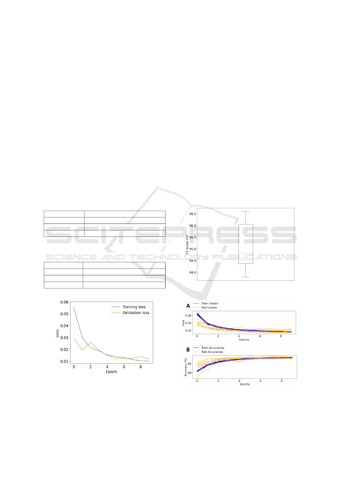
Epoch Optimisation for the Grouped CNN. From

Figure 6, the optimum number of epochs for the

grouped CNN architecture, using the heatmap feature

vectors, was determined to be 10; this is where both

the training and validation loss begin to level out, im-

plying that any further training would not improve the

model’s performance.

Analysing Customer Behaviour Using Simulated Transactional Data

505

Model Performances. From Table 1, when predict-

ing the class of the heatmaps in the test dataset, the

grouped CNN model performed substantially better

than the image-baseline model and the single kernel

model, achieving an F1 score of 94.3% (p = 2e

−5

≪

0.01, paired bootstrap test).

Thus, the improved performance of the grouped

CNN model is likely not accidental. Moreover, from

Table 2 and Table 1 for the single and grouped CNN

architectures, the heatmap feature vectors showed far

greater performances on the test set than the con-

ventional feature vectors. Lastly, all the models per-

formed better at classifying the test set than the stan-

dard K-NN baseline that is typically used in the liter-

ature (Fawaz et al., 2019).

Figure 7 shows that the grouped CNN model using

heatmap feature vectors achieved a very high F1 score

of 94.8% during cross-validation, consistent with the

test set result. The cross-validation history shown in

Figure 8 indicates that there was minimal overﬁtting

throughout the cross-validation process.

Table 1: Performance on the test set using heatmap features.

Model Mean F1 score on test set (n=10)

Image-Baseline 78.6%

Single CNN 86.1%

Grouped CNN 94.3%

Table 2: Performance on the test set using conventional fea-

ture vectors.

Model Mean F1 score on test set (n=10)

K-NN 25.7%

Single CNN 80.4%

Grouped CNN 77.0%

Figure 6: Loss versus epoch for grouped CNN using

heatmap feature vectors.

4.3 Risk Score Algorithm Results

Hyperparameter Value Selection. The ranked im-

portance of the hyperparameters used in Equation 2

can be seen in Table 3. The values α, δ and ε, which

weigh the importance of the maximum width, median

normalised sum spending and median normalised

standard deviation, respectively, were all ranked high-

est. This is because the length of consecutive daily

spending (a) was seen to be equally important as the

average spending in a contour (d), and the average

variability in a day’s spending ( f ). The least impor-

tant variable was determined to be the area (c), so

its corresponding hyperparameter γ was ranked as 3.

While the area of a contour gives an idea of the num-

ber of payments present within it, the other contour

statistics have a more direct relationship with risky

spending behaviour. Lastly, consecutive spending on

the same day of the week (b) was seen as a greater

indicator of risky spending behaviour than the area of

a contour (c) but less signiﬁcant than a, d or f , so its

corresponding hyperparameter β was ranked as 2.

Figure 7: 10-fold CV F1 score results. Median = 94.8%.

IQR = 1.7%.

Figure 8: 10-fold CV history. A: Loss vs epoch. B: Accu-

racy vs epoch.

ICAART 2023 - 15th International Conference on Agents and Artiﬁcial Intelligence

506

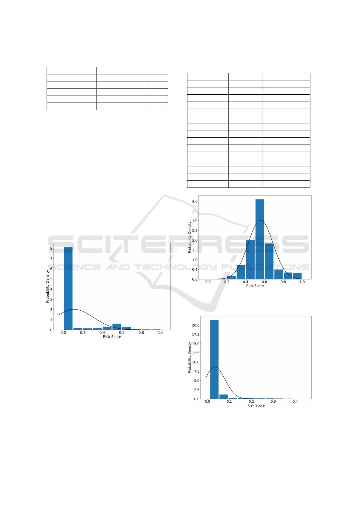
Table 3: Hyperparameter importance (1 is highest).

Contour statistic Hyperparameter Rank

a α 1

b β 2

c γ 3

d δ 1

f ε 1

Analysing the Distribution of Risk Scores. The

overall distribution of risk scores, for the accounts in

the test set, can be seen in Figure 9. This distribu-

tion is heavily positively skewed and does not approx-

imate a normal distribution very well. Moreover, it is

composed of two overlapping distributions contain-

ing the Tetris and Non-Tetris risk scores, which can be

seen in Figures 10 and 11. The Tetris scores better ap-

proximate a normal distribution, while the Non-Tetris

scores are positively skewed. Furthermore, due to the

class imbalance in the dataset (see Section 4.1), when

these distributions are combined, the Non-Tetris data

dominates causing the overall distribution in Figure 9

to be heavily right-skewed. Finally, using Equation 4

and the overall distribution statistics (see Figure 9), a

cut-off point for risky spending behaviour was calcu-

lated to be 0.512.

Figure 9: Normalised distribution of risk scores in test set

with approximate normal distribution overlaid. µ = 0.112,

σ = 0.20.

Risk Scores per Spending Category. Table 4

shows a series of risk scores for each category in an

example customer’s transactional history along with

a risky spending label. This label is based on the risk

threshold calculated in Section 4.3. In the case of this

individual, they spend impulsively in the online shop,

clothing shop, supermarket, and takeaway categories.

Table 4: Risk scores for an example user in each category

with corresponding risky spending behaviour labels.

Category Risk Score Risky Spending?

Finances 0.018 N

Entertainment 0.017 N

Online shop 0.536 Y

Exercise 0 N

Personal care 0.417 N

Clothing shop 0.523 Y

Restaurant 0 N

Cafe 0 N

Supermarket 0.59 Y

Education 0.062 N

Home Shop 0.026 N

Pub/Bar 0 N

Takeaway 0.928 Y

Sports shop 0 N

Family 0 N

Figure 10: Normalised distribution of risk scores for the

Tetris labelled data in the test set with approximate normal

distribution overlaid.

X = 0.558, σ = 0.131.

Figure 11: Normalised distribution of risk scores for the

Non-Tetris labelled data in the test set with approximate

normal distribution overlaid.

X = 0.034, σ = 0.046.

Analysing Customer Behaviour Using Simulated Transactional Data

507

5 DISCUSSION

5.1 Critical Findings

From Section 4.2, when classifying the heatmap im-

ages the grouped CNN model signiﬁcantly outper-

formed the baseline models and the single kernel

model on the test set, as well as during 10-fold cross-

validation of the training set. This ﬁnding shows that

when analysing the heatmap representation, the use of

a CNN with grouped convolution (Krizhevsky et al.,

2012), global max pooling (Lin et al., 2013) and fo-

cal loss (Lin et al., 2017) outperforms the alternative

conﬁgurations. This is likely due to the complex geo-

metric features present in the heatmap representation,

which can be difﬁcult for a more conventional CNN,

like the one used in Butler et al. (2022), to classify.

Therefore, these results satisfy the ﬁrst aim of this

study. Section 4.2 also shows that the heatmap rep-

resentation is superior to a conventional time series

representation in both the single and grouped CNN

models, satisfying the second aim of this study. Fur-

thermore, from Section 4.3, contour detection, a con-

temporary image analysis technique, was used to suc-

cessfully deconstruct the heatmap images into their

geometric components and derive information from

them, thereby satisfying the third aim of this study.

Section 4.3 demonstrated an algorithm for overall

risk score in several categories using the heatmap rep-

resentation. The overall distribution of risk scores in

the test set (Figure 9), is heavily positively skewed,

which at ﬁrst glance implies the model is not discrim-

inating well between different levels of risk. How-

ever, this distribution is in fact composed of two over-

lapping distributions, one containing the Tetris risk

scores and one containing the Non-Tetris risk scores

(see Figures 10 and 11). The Non-Tetris risk score

distribution is highly right-skewed, and this is likely

because the risk score equation (Equation 2) weights

its output by the probability of a Tetris classiﬁca-

tion; hence causing the Non-Tetris labelled data to

have far lower scores. This aligns with our aims, as

if a heatmap is labelled as Non-Tetris, it means the

heatmap lacks clear geometric features, which are as-

sociated with an underlying spending behaviour in

a given category and are a key indicator of impul-

sive spending. Consequently, it makes sense for Non-

Tetris heatmaps to have risk scores closer to 0 as these

heatmaps are far less likely to contain risky spending

behaviours.

On the other hand, the Tetris distribution in Figure

10 better approximates a normal distribution, which

shows that the risk score algorithm can effectively

distinguish between the different levels of risk in the

Tetris labelled data. Therefore, the risk score algo-

rithm appears to be a promising approach for cal-

culating risk because it discriminated risk effectively

within the Tetris heatmaps and because the high pos-

itive skew in the overall distribution was a conse-

quence of the class imbalance (see Section 4.3) and

the very low risk scores of the Non-Tetris data.

Lastly, if a ﬁnancial product is strongly related to

a particular risk score category, this value and corre-

sponding label can be used to inform a retail bank of

that customer’s risk. For example, it would not be ap-

propriate to offer a customer a cashback card focused

on clothes shopping if the output of this algorithm

shows that the individual is spending impulsively in

that particular category. Therefore, this algorithm sat-

isﬁes the fourth aim of this paper.

5.2 Limitations and Recommendations

A key limitation of this study is that the utilised

dataset did not have any golden labels for the ﬁnal

risk score. As a result, it is difﬁcult to validate these

scores without involving the author’s bias. However,

the inclusion of adjustable hyperparameters (see Sec-

tion 3.7.2) allows for controlling and mitigating this

bias. An individual with access to data with golden

labels will be able to adjust these parameters accord-

ingly and validate the algorithm. Consequently, it is

recommended that if the user of this algorithm pos-

sesses a dataset with golden labels that are compa-

rable to the risk scores generated by this algorithm,

they should use these to validate their hyperparameter

value selections and the calculated impulsive spend-

ing threshold, and thus limit the integration of their

own bias into the algorithm. Therefore, the algorithm

produced in this study is a proof of concept to demon-

strate how ABM and applied artiﬁcial intelligence can

be used for the purpose of KYC and should not be di-

rectly implemented into a KYC pipeline. In addition,

as the dataset used in this study is synthetic, the anal-

ysis in relation to risk in this study (see Section 4.3)

will need to be validated through the deployment of

these techniques on real customer data.

Another limitation is that the transaction cate-

gories in this study were created by manually choos-

ing several categories that included all the available

vendors in the dataset. In practice, however, this is

not feasible, as developing a rules-based sorting sys-

tem for every possible vendor becomes problematic

due to the volume and variability in the transactions a

bank receives (UK Finance, 2022).

ICAART 2023 - 15th International Conference on Agents and Artiﬁcial Intelligence

508

5.3 Ethical Considerations

An ethical risk of the proposed algorithm is that the

risk scores could unintentionally highlight subsec-

tions of the population. This is because risky spend-

ing behaviour could be a result of compulsive buying

disorder (CBD), deﬁned as “excessive shopping cog-

nitions and buying behaviour that leads to distress or

impairment” (Black, 2007). Research has shown that

CBD is associated with attention deﬁcit hyperactivity

disorder (ADHD) (Brook et al., 2015). Thus, it may

be possible to predict neurodiversity from these risk

scores. Therefore, any further research into this al-

gorithm’s application must be solely focused on KYC

and customer-safeguarding to avoid identifying vul-

nerable members of the population.

6 CONCLUSIONS

This paper proposed a method for satisfying the cus-

tomer safeguarding aspect of KYC by representing

ﬁnancial transactions as a heatmap, analysing the

heatmap using a CNN and contour detection, then

outputting a risk score and impulsivity label for each

spending category. These risk scores, along with their

corresponding labels, can be used to safeguard cus-

tomers from unsuitable ﬁnancial products. In Sec-

tion 4.2, we showed that a CNN with grouped con-

volution, global max pooling, and binary focal cross-

entropy loss outperforms alternative conﬁgurations

when analysing the complex geometric features in the

heatmap representation. This model was able to dis-

tinguish between the heatmaps with a clear geomet-

ric structure (“Tetris”) and those without , yielding

an F1 score of 94.8% during 10-fold cross-validation,

which far exceeded the baseline models and the sin-

gle kernel model (Butler et al., 2022). The heatmap

representation also exceeded the performance of the

conventional feature vectors when evaluating both the

single and grouped CNN architectures. This work

demonstrates how agent-based modelling can pro-

duce datasets that applied artiﬁcial intelligence can

use to aid ﬁrms in adhering to KYC regulation.

6.1 Future Work

In Sinanc et al. (2021), the GAF image-transform

technique (Wang and Oates, 2015) has demonstrated

high effectiveness at predicting credit card fraud in

transactional data, and may also be applicable to the

customer-safeguarding aspect of KYC. One way to

achieve this is to combine GAF with a heatmap rep-

resentation where, instead of R, G and B layers (see

Section 3.3), each “pixel” is instead composed of a

GAF representation of that day’s spending. In our

current approach, the G and B layers aggregate a day’s

spending into a single value, thus removing the time

dimension and resulting in the loss of some infor-

mation. This new design, however, would maintain

the time series nature of an individual day’s spending

while preserving the image’s interpretability by struc-

turing the days in a heatmap.

Another avenue of future work is the use of natural

language processing (NLP) (Navigli, 2009) to cate-

gorise transactions as opposed to the rules-based sort-

ing method used in this study. A rules-based method

would be unable to handle the variety and volume of

vendor names that retail banks process (see Section

5.2). However, a theoretical NLP system could use

Regex (Aho, 1990) to extract key components of the

vendor names before using a technique such as latent

Dirichlet allocation (LDA) (Blei et al., 2003) to cat-

egorise them. This would allow a greater variety of

vendor names to be processed, thus overcoming the

second limitation discussed in Section 5.2.

REFERENCES

Aho, A. V. (1990). Algorithms for ﬁnding patterns in

strings. In Leeuwen, J. V., editor, Algorithms and

Complexity, Handbook of Theoretical Computer Sci-

ence, chapter 5, pages 255–300. Elsevier, Amsterdam.

Bagnall, A., Lines, J., Bostrom, A., Large, J., and Keogh,

E. (2017). The great time series classiﬁcation bake

off: a review and experimental evaluation of recent

algorithmic advances. Data Mining and Knowledge

Discovery, 31(3):606–660.

Bagnall, A., Lines, J., Hills, J., and Bostrom, A. (2016).

Time-series classiﬁcation with cote: The collective

of transformation-based ensembles. In 2016 IEEE

32nd International Conference on Data Engineering

(ICDE), pages 1548–1549.

Basha, S. S., Dubey, S. R., Pulabaigari, V., and Mukherjee,

S. (2020). Impact of fully connected layers on per-

formance of convolutional neural networks for image

classiﬁcation. Neurocomputing, 378:112–119.

Bishop, C. M. (2016). Pattern recognition and machine

learning. Springer-Verlag, New York.

Black, D. W. (2007). A review of compulsive buying disor-

der. World Psychiatry, 6(1):14–18.

Blei, D. M., Ng, A. Y., and Jordan, M. I. (2003). Latent

dirichlet allocation. Journal of machine Learning re-

search, 3:993–1022.

Bowerman, B. L. and O’Connell, R. T. (1993). Forecast-

ing and time series: An applied approach. 3rd. ed.

Duxbury Press.

Britannica, The editors of Encyclopedia (2022). Encyclo-

pedia britannica: Tetris. https://www.britannica.com/

topic/Tetris.

Analysing Customer Behaviour Using Simulated Transactional Data

509

Brook, J. S., Zhang, C., Brook, D. W., and Leukefeld, C. G.

(2015). Compulsive buying: Earlier illicit drug use,

impulse buying, depression, and adult ADHD symp-

toms. Psychiatry Research, 228(3):312–317.

Butler, R., Hinton, E., Kirwan, M., and Salih, A. (2022).

Customer behaviour classiﬁcation using simulated

transactional data. Proceedings of the European Mod-

eling & Simulation Symposium, EMSS.

Chen, T.-H. (2020). Do you know your customer? bank risk

assessment based on machine learning. Applied Soft

Computing, 86:105779.

Culjak, I., Abram, D., Pribanic, T., Dzapo, H., and Cifrek,

M. (2012). A brief introduction to opencv. In

2012 Proceedings of the 35th International Conven-

tion MIPRO, pages 1725–1730.

Efron, B. and Tibshirani, R. J. (1993). An Introduction to

the Bootstrap. Springer US, Boston, MA.

Fawaz, H. I., Forestier, G., Weber, J., Idoumghar, L., and

Muller, P.-A. (2019). Deep learning for time series

classiﬁcation: a review. Data Mining and Knowledge

Discovery, 33(4):917–963.

Financial Conduct Authority (2004). Cob 5.2 Know Your

Customer – fca handbook. https://www.handbook.fca.

org.uk/handbook/COB/5/2.html?date=2007-10-31.

Gong, X.-Y., Su, H., Xu, D., Zhang, Z.-T., Shen, F., and

Yang, H.-B. (2018). An overview of contour detection

approaches. International Journal of Automation and

Computing, 15(6):656–672.

GOV.UK (2016). ’Know Your Customer’ guid-

ance. https://www.gov.uk/government/

publications/know-your-customer-guidance/

know-your-customer-guidance-accessible-version.

Hackshaw, A. (2008). Small studies: Strengths

and limitations. European Respiratory Journal,

32(5):1141–1143.

Hatami, N., Gavet, Y., and Debayle, J. (2017). Classiﬁ-

cation of time-series images using deep convolutional

neural networks.

Hinton, G. E., Srivastava, N., Krizhevsky, A., Sutskever, I.,

and Salakhutdinov, R. R. (2012). Improving neural

networks by preventing co-adaptation of feature de-

tectors.

Joseph, V. R. (2022). Optimal ratio for data splitting. Sta-

tistical Analysis and Data Mining: The ASA Data Sci-

ence Journal, 15(4):531–538.

Khandani, A. E., Kim, A. J., and Lo, A. W. (2010).

Consumer credit-risk models via machine-learning

algorithms. Journal of Banking & Finance,

34(11):2767–2787.

Koehler, M., Tivnan, B., and Bloedorn, E. (2005). Gen-

erating fraud: Agent based ﬁnancial network model-

ing. In Proceedings of the North American Associa-

tion for Computation Social and Organization Science

(NAACSOS 2005). Notre Dame, IN, page 5.

Kohavi, R. (1995). A study of cross-validation and boot-

strap for accuracy estimation and model selection. In

Proceedings of the 14th International Joint Confer-

ence on Artiﬁcial Intelligence - Volume 2, IJCAI’95,

page 1137–1143, San Francisco, CA, USA. Morgan

Kaufmann Publishers Inc.

Krizhevsky, A., Sutskever, I., and Hinton, G. E. (2012).

Imagenet classiﬁcation with deep convolutional neu-

ral networks. In Proceedings of the 25th Interna-

tional Conference on Neural Information Processing

Systems - Volume 1, NIPS’12, page 1097–1105, Red

Hook, NY, USA. Curran Associates Inc.

LeCun, Y., Bottou, L., Bengio, Y., and Haffner, P. (1998).

Gradient-based learning applied to document recogni-

tion. Proceedings of the IEEE, 86(11):2278–2324.

Lin, M., Chen, Q., and Yan, S. (2013). Network in network.

arXiv preprint arXiv:1312.4400.

Lin, T.-Y., Goyal, P., Girshick, R., He, K., and Doll

ar, P.

(2017). Focal loss for dense object detection.

Lines, J., Taylor, S. L., and Bagnall, A. (2016). Hive-cote:

The hierarchical vote collective of transformation-

based ensembles for time series classiﬁcation. 2016

IEEE 16th International Conference on Data Mining

(ICDM), pages 1041–1046.

Marwan, N. (2011). How to avoid potential pitfalls in recur-

rence plot based data analysis. International Journal

of Bifurcation and Chaos, 21(04):1003–1017. Pub-

lisher: World Scientiﬁc Publishing Co.

Navigli, R. (2009). Word sense disambiguation: A survey.

ACM Comput. Surv., 41(2).

Ogonsola, F. and Pannifer, S. (2017). AMLD4/

AMLD5 KYCC: Know your compliance costs.

https://www.fstech.co.uk/fst/mitek/Hyperion-

Whitepaper-Final-for-Release-June2017.pdf.

PassFort (2015). Passfort. https://www.passfort.com/.

Ross, S. M. (2009). DESCRIPTIVE STATISTICS. In In-

troduction to Probability and Statistics for Engineers

and Scientists, pages 9–53. Elsevier.

Sinanc, D., Demirezen, U., and Sa

gıro

glu, c. (2021). Ex-

plainable credit card fraud detection with image con-

version. ADCAIJ: Advances in Distributed Computing

and Artiﬁcial Intelligence Journal, 10(1):63–76.

Suzuki, S. and Abe, K. (1985). Topological structural anal-

ysis of digitized binary images by border following.

Computer Vision, Graphics, and Image Processing,

30(1):32–46.

UK Finance (2022). Card spending update for au-

gust 2022. https://www.ukﬁnance.org.uk/data-and-

research/data/card-spending.

Umer, M., Imtiaz, Z., Ullah, S., Mehmood, A., Choi, G. S.,

and On, B.-W. (2020). Fake news stance detection

using deep learning architecture (cnn-lstm). IEEE Ac-

cess, 8:156695–156706.

Wang, Z. and Oates, T. (2015). Spatially encoding temporal

correlations to classify temporal data using convolu-

tional neural networks.

Wolford, B. (2016). Regulation (EU) 2016/679 of the Euro-

pean Parliament and of the Council of 27 April 2016

on the protection of natural persons with regard to the

processing of personal data and on the free movement

of such data, and repealing Directive 95/46/EC (Gen-

eral Data Protection Regulation) (Text with EEA rele-

vance).

Xie, S., Girshick, R., Doll

ar, P., Tu, Z., and He, K. (2016).

Aggregated residual transformations for deep neural

networks.

ICAART 2023 - 15th International Conference on Agents and Artiﬁcial Intelligence

510

REFERENCES

Aho, A. V. (1990). Algorithms for finding patterns in