Coevolving Hexapod Legs to Generate Tripod Gaits

Cameron L. Angliss and Gary B. Parker

Connecticut College, New London, CT, U.S.A.

Keywords:

Hexapod, Genetic Algorithm, Neural Network, Multiagent, Coevolve, Learning, Simulation.

Abstract:

This research is the ﬁrst step in new research that is investigating the use of an extensive neural network (NN)

system to control the gait of a hexapod robot by sending speciﬁc position signals to each of the leg actuators.

The system is highly distributed with nerve clusters that control each leg and no central controller. The intent

is to create a more biologically-inspired system and one that has the potential to dynamically change its gait

in real-time to accommodate for unforeseen malfunctions. We approach the evolution of this extensive NN

system in a unique way by treating each of the legs as an individual agent and using cooperative coevolution to

evolve the team of heterogeneous leg agents to perform the task, which in this initial phase is walking forward

on a ﬂat surface. When tested using a simulated hexapod robot modeled after an actual robot, this new method

reliably produced a stable tripod gait.

1 INTRODUCTION

Within the ﬁeld of robotics, legged robots constitute a

signiﬁcant challenge. Many forms of legged robots

have been considered such as the hexapod, a six-

legged robot. A tripod gait is a stable and efﬁcient

hexapod gait (Lee et al., 1988) in which the front-left,

middle-right, and back-left legs move synchronously

in a stepping motion, and the other three legs move

synchronously with one another and exactly a half-

cycle behind the former three legs. Thus, it is feasible

for one to hard-code the leg motions of a hexapod to

produce its optimal gait. However, hard-coded hexa-

pod gaits are tedious to write, subject to human error,

and less capable of adapting to changes in the robot’s

physical capabilities or its environment. These issues

motivate the use of automation to generate hexapod

gaits.

Work has been done to automate the generation

of hexapod gaits using evolutionary computation. In

most of these works, gaits were learned using a sin-

gle central controller or control program. Exam-

ples include (Gallagher et al., 1996) who used a ge-

netic algorithm (GA) to learn the weights of a neu-

ral network, (Parker and Rawlins, 1996) who used

cyclic genetic algorithms (CGAs) to learn the for-

ward/back and up/down motions of the legs in coor-

dination, (Spencer, 1993) who used genetic program-

ming, (Barfoot et al., 2006) who compare the use of

GAs and reinforcement learning algorithms to evolve

cellular automata for control, (Lewis et al., 1993) who

evolved complex motor pattern generators with a GA,

(Juang et al., 2010) who evolved recurrent neural net-

works using symbiotic species-based particle swarm

optimization, (Earon et al., 2000) who evolve cellular

automata for control using a GA, (Vice et al., 2022)

who used an evolutionary algorithm to evolve param-

eters for a hexapod model that used a Robot Oper-

ating System clock that created a continuous sinu-

soidal wave, and (Belter and Skrzypczy

nski, 2010)

who applied progressively more biologically-inspired

constraints on the set of possible leg movements of

the hexapod throughout its evolution.

In these works, the entire control system was

evolved as one chromosome and/or the signals sent

to the legs were binary directional commands (move

forward or backward). Our work differs from these

in that there is an individual NN controller evolved

for each leg of the hexapod that outputs speciﬁc posi-

tion commands to its servos. There are a total of 16

horizontal and vertical position commands the con-

troller can make. In addition to specifying the limits

of the leg movement, this allows the control system to

vary the rate of leg movement – the front-left leg can

be moving at full speed while the middle-right leg is

moving at half speed. Although more complicated,

this gives the control system additional ﬂexibility for

atypical situations requiring an atypical gait.

Previous works that used nerve clusters to give

hexapod legs speciﬁc-position control are of signiﬁ-

Angliss, C. and Parker, G.

Coevolving Hexapod Legs to Generate Tripod Gaits.

DOI: 10.5220/0011896200003393

In Proceedings of the 15th International Conference on Agents and Artiﬁcial Intelligence (ICAART 2023) - Volume 3, pages 1063-1071

ISBN: 978-989-758-623-1; ISSN: 2184-433X

 2023 by SCITEPRESS – Science and Technology Publications, Lda. Under CC license (CC BY-NC-ND 4.0)

1063

cant relevance to this paper; in these works, hexapod

gaits were learned incrementally in two phases. In the

ﬁrst phase, an individual leg cycle was learned by ei-

ther using a CGA (Parker, 2001) or by using a GA to

evolve the weights of a neural network (Parker and Li,

2003), both of which yielded output that directed the

desired positions of the servos every 25 milliseconds.

In the second phase, a GA was used to learn the co-

ordination of the hexapod’s legs (Parker, 2001). The

research presented in this paper extends the work of

(Parker and Li, 2003) to full-hexapod control without

necessitating the incremental approach described in

(Parker, 2001). Each leg of the hexapod has one of its

position sensors connected to all the other legs to al-

low for inter-leg communication, and the legs are co-

operatively coevolved so they learn in parallel while

interfacing through neural connections to the posi-

tional sensors of the other legs. This method yields

decentralized hexapod gaits operated by six cooperat-

ing leg controllers, as opposed to the centralized con-

troller found in previous works. Since the control is

not localized in one speciﬁc location on the physical

hexapod, we would no longer need to be concerned

with the main control unit being damaged or malfunc-

tioning since the robot no longer relies entirely on any

one single control unit.

This research involves the initial phase of the

development of this highly distributed NN system,

where each leg has a nerve cluster that receives data

from the position sensors of the other legs and con-

trols that leg’s movement. This is intended to create

a more biologically inspired system that has the po-

tential to adapt the gait due to changes in the capa-

bilities of one or multiple of the hexapod’s legs. The

idea of the leg nerve clusters is loosely modeled after

(Beer, 1990), except that only the output neurons of

any given nerve cluster have a speciﬁc function and

the control is more precise. The entire NN system

in our robot requires 2070 bits to represent all of the

values, thresholds, and weights. We use a GA, but the

size of the chromosome makes evolution very difﬁcult

for a single GA. To address this issue, we use cooper-

ative coevolutionary algorithms (CCAs), which were

described in (Potter and Jong, 1994) to handle evolu-

tions requiring large chromosomes. In addition, using

CCAs gives us the opportunity to treat each leg as an

individual agent (similar to (Potter et al., 2001)) ex-

cept that in our work there is a requirement for coop-

erative coevolution of a team of six heterogeneous leg

agents, which is an interesting problem since no two

of the agents have the same controller as they are all in

different positions on the robot. The work done at this

point was all completed in simulation, but the simula-

tion was based on a speciﬁc robot, which was already

conﬁgured with individual controllers for each leg.

This robot also has a central controller, which was

used in past research, but for this research, it was not

used. In this initial stage of the research, the contri-

bution is to apply cooperative coevolution to a unique

task requiring six individual agents and to show that

our NN system is capable of generating reasonable

gaits for a fully functional robot walking forward on

a ﬂat surface.

The paper is structured as follows: Section 2 dis-

cusses the speciﬁc methods used to coevolve hexa-

pod gaits; Section 3 discusses the results that those

techniques yielded; Section 4 makes concluding re-

marks and discusses potential future work; and Sec-

tion 5 provides a mathematical derivation for the yaw

equation used in Section 2.4.

2 SYSTEMS/TECHNIQUES

A detailed overview will now be given demonstrating

how neural networks and genetic algorithms are uti-

lized in this research.

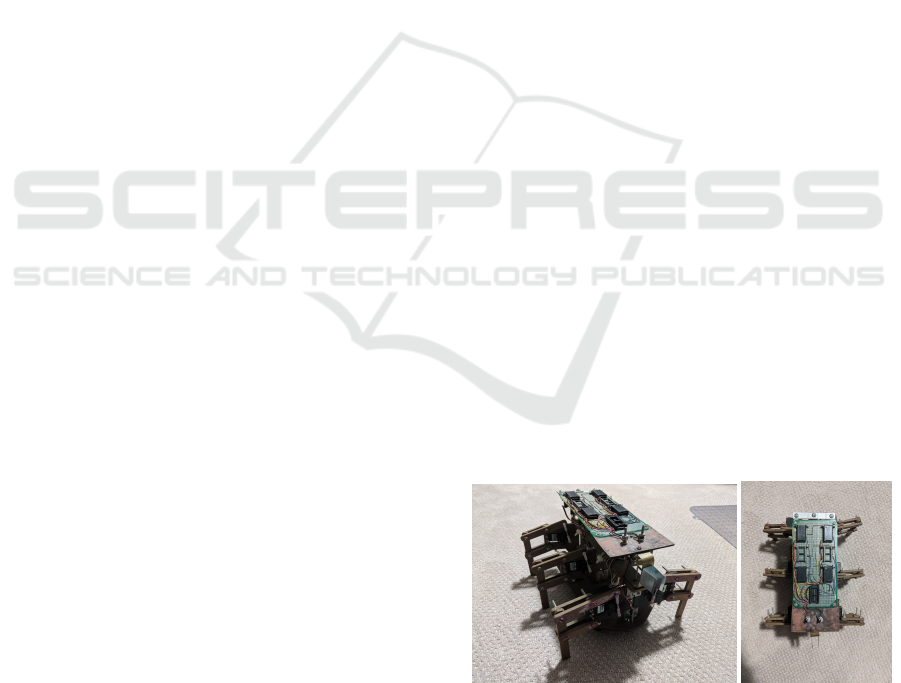
2.1 Physical Hexapod

The hexapod used (Figure 1) to create our model is

a servobot conﬁgured with 7 BS2 BASIC Stamps for

control and two servos per leg to provide vertical and

horizontal degrees of freedom. Six of the BASIC

Stamps are in 1-to-1 correspondence with the hexa-

pod’s six legs, and each controller is responsible for

controlling its leg’s motion. The other BASIC Stamp

is meant to coordinate the leg motions into a meaning-

ful hexapod gait; however, that controller is not nec-

essary for this research, as the six legs are learning

to coordinate among themselves without a dedicated

central coordination controller.

Figure 1: Hexapod Modeled in Simulation.

Every 25 milliseconds, an electrical signal is sent

from each BASIC Stamp to its leg’s vertical and hor-

izontal servos, and the pulse width of that signal is

what determines what position it will attempt to reach.

ICAART 2023 - 15th International Conference on Agents and Artiﬁcial Intelligence

1064

However, just because a servo receives a signal telling

it to go to a position doesn’t mean it’s physically pos-

sible to do so. The servo can only turn so much within

the 25-millisecond span before it receives another sig-

nal, and this depends on what the leg’s initial momen-

tum was before the servo received that signal. For

example, if the leg is moving backward and is almost

fully extended backward, and then receives a direc-

tion to extend all the way forward, it certainly won’t

complete this command in a 25-millisecond span, and

it will do substantially worse in that 25-millisecond

span than if it was initially moving forward instead

of backward since it would already have some mo-

mentum. In Section 3.4, the ideas of momentum and

positional requests are formalized mathematically for

the sake of implementing a simulation.

2.2 Genetic Algorithm Coevolution

A genetic algorithm, ﬁrst devised by John H. Holland

(Holland, 1992), is a computational tool that evolves

a population of solutions to a given problem over a

number of generations. The solutions to the problem

in question are represented as chromosomes, which

are strings of 0’s and 1’s. The solutions are tested and

given a numeric ﬁtness value based on a user-deﬁned

metric of what counts as good and bad for the solu-

tion. Total ﬁtness is then calculated, which is the sum

of all ﬁtness values of all the solutions in the current

population. The fraction of a solution’s ﬁtness value

over the total ﬁtness of the population represents the

probability of that solution being selected for repro-

duction.

After two solutions are selected, we derive a child

from them. First, the parents’ chromosomes are

crossed over, which means that there’s a 50% chance

that either parent will pass down a given piece of their

chromosome to the child. The chromosomes are seg-

mented into parts so that a given segment wholly con-

tains a given piece of the solution. For example, if

the chromosome from index 5 to index 10 deﬁnes a

certain characteristic of the solution, then we refrain

from fracturing that trait, and instead, deﬁne index 5

through 10 to be an atomic unit of the chromosome.

Once all of the components of a complete chromo-

some have been passed down from the parents, the

child’s chromosome is then mutated based on a muta-

tion rate M ∈ [0,1], which represents the probability

that a bit of the child’s chromosome will ﬂip from 0

to 1 or vice versa. The resulting child is appended to a

list of children. This process iterates until the number

of children is equal to the parent population, at which

point the child population overwrites the parent pop-

ulation. The child population then creates a new child

population by the same procedure, and this process it-

erates for some number of generations. The intention

is that the solutions will begin to converge toward the

optimal solution.

The structure of the genetic algorithm used in this

work is atypical and takes inspiration from (Potter and

Jong, 1994), (Potter et al., 2001), (Wiegand et al.,

2001). Instead of having each hexapod representa-

tion as an individual in the population being evolved

from generation to generation, we have constructed 6

genetic algorithms coevolving each of the 6 legs of

the hexapod. For example, in one of the genetic al-

gorithms, all members of its population are legs that

identify as the front-right leg of the hexapod.

In the center of the evolution is a reference hexa-

pod. The reference hexapod is composed of one rep-

resentative individual from each of the 6 genetic algo-

rithms, each of which is the highest-performing leg of

their respective populations. Every G generations, the

reference hexapod undergoes an update in which the

best individuals from each population replace the cur-

rent representatives in the reference hexapod. How-

ever, when learning ﬁrst starts at generation 0, the ref-

erence hexapod is initialized randomly.

To get the ﬁtness of an individual leg in a popu-

lation, the leg to be tested is attached to the reference

hexapod at the position that it identiﬁes as (if it comes

from the forward-left leg population, it would replace

the reference leg’s forward-left leg). The leg’s ﬁtness

is then set equal to the ﬁtness of the resulting hexapod.

Every generation, all P legs from all 6 populations are

evaluated individually in this way. Additionally, once

the reference hexapod has been updated, all legs from

all populations must have their ﬁtnesses evaluated so

that their ﬁtnesses are relative to the newly-updated

reference hexapod.

Figure 2 illustrates the role of the reference hexa-

pod with a ﬂowchart. The arrows from the GA blocks

to the Reference Hexapod block signify that each leg

of the reference hexapod is updated every G gener-

ations by the corresponding GA’s strongest current

leg individual. The arrows from the Reference Hexa-

pod block to the GA blocks signify that the reference

hexapod is used to provide a common basis for test-

ing the legs of all six GAs, in which testing is done by

attaching the leg to be tested at its designated position

on the reference hexapod and evaluating the gait of

the resulting hexapod in a simulation. It can be seen

from Figure 2 that the reference hexapod is an inter-

face through which the six GAs are able to coordinate

with each other.

Additionally, all 6 GAs implement elitism, which

makes the strongest individual of a population survive

to the next generation, as opposed to regular individ-

Coevolving Hexapod Legs to Generate Tripod Gaits

1065

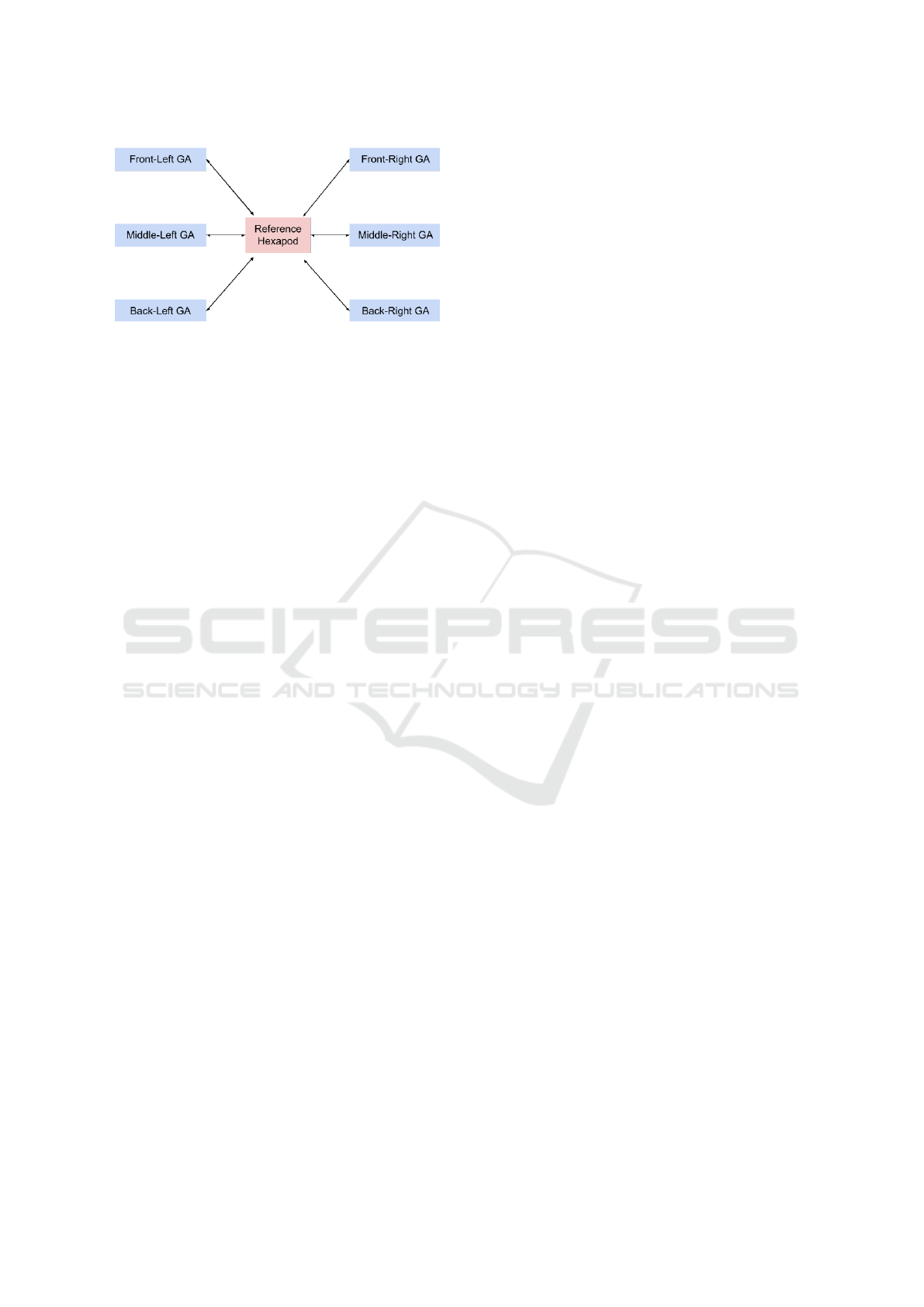
Figure 2: Arrows to the reference hexapod represent that it

is composed of representative legs from each GA; the ar-

rows in the opposite direction show that each GA uses the

Reference Hexapod to test its population.

uals whose lifespan is always exactly one generation.

When another individual surpasses the strongest agent

in the population, they become the new elite mem-

ber of the population, and the prior elite is guaranteed

to die when the next population of offspring is com-

pleted.

2.3 Neural Network Architecture

A neural network is a computational decision-making

tool that receives data as input and returns an output,

and is inspired by the neural systems of animals and

humans. Neural networks are universal function ap-

proximators, meaning that if a neural network is al-

lowed to grow unboundedly in its complexity, it can

converge to any real-valued function with arbitrary

precision. In programs, a NN can be represented as

a graph of nodes and edges, where the nodes repre-

sent neurons, and the edges represent connections be-

tween the neurons. A neuron contains a value that is

subject to change every time the neurons in the neural

network ﬁre. When they ﬁre, each neuron accumu-

lates the linear combination of each neuron’s value

that is connected to it by an edge multiplied by the

weights of the edges going from those other neurons

to the neuron in question. That accumulation is then

run through an activation function, and the output of

that activation function replaces that neuron’s current

value. This happens all throughout the neural network

iteratively.

The neural networks used in this paper are not tra-

ditional feed-forward neural networks. All the neu-

rons are fully connected, meaning each neuron has

a weighted connection to every other neuron in the

network, including itself. Also, there are three sen-

sors that send their data selectively to certain neurons

in the neural network through weighted connections.

Two of the neurons are selected to be output neurons,

but the distinction between them and ”hidden” neu-

rons is blurred in our model since the output neurons

are also receiving input from sensors. Also, externally

from a leg’s neural network, other legs’ neural net-

works send their sensor data through weighted con-

nections to that leg’s neurons. Section 3.1 goes into

more detail on how the NN architecture is designed.

The controller for the hexapod is composed of 6

neural networks for each of its 6 legs, each contain-

ing N neurons, where N ≥ 2, since we at least need

the 2 output neurons to produce the next vertical and

horizontal position signals for the leg.

Each leg of the hexapod has 3 sensors. Sup-

pose we are considering leg l of the hexapod, where

1 ≤l ≤6. Deﬁne o to be a function that maps a sensor

to its current output (a value of 0 or 15). This leg fea-

tures a forward sensor, back sensor, and down sensor,

denoted F

, B

, and D

, where

o(F

) =

(

15, leg is fully forward

0, otherwise

(1)

o(B

) =

(

15, leg is fully back

0, otherwise

(2)

o(D

) =

(

15, leg is fully down

0, otherwise

(3)

Let S

= {F

} be the set of all sensors of leg l.

Also, let D

= {D

...,D

}−{D

} be the set of

all the hexapod’s legs’ down sensors except for leg l’s

down sensor.

Let n represent some neuron of a leg, where

1 ≤ n ≤ N. If n ∈ {3,4,...N}, the neuron is a hid-

den neuron of the leg’s neural network; otherwise,

n ∈ {1,2} and the neuron is an output neuron. Both

types of neurons will store a value v ∈ {0, 1, 2,...15},

a threshold t ∈{−511,−510,. . . 511}, a threshold s ∈

{−255,−254,...255}, and N weights {w

m→n

| 1 ≤

m ≤ N}. Note that all neurons share connections

with each other. Hidden neurons store an additional

5 sensor weights, w

s→n

, where s ∈ D

, whereas out-

put neurons store an additional 3 sensor weights,

s→n

, where s ∈ S

. All weights w have that w ∈

{−15,−14,...15}.

A visual of the neural network architecture is

given in Figure 3. Note that in reality, every leg’s

down sensor sends its output to the hidden neurons

of every other leg’s neural network, but in order to

simplify this, Figure 3 captures all the inputs taken in

by only one of the neural networks.

Formally, for neuron n of leg l, the accumulation

function of n can be deﬁned as

A(l, n) =

∑

m=1

m→n











∑

s∈S

o(s)w

s→n

, n ≤ 2}

∑

s∈D

o(s)w

s→n

, n > 2}

(4)

ICAART 2023 - 15th International Conference on Agents and Artiﬁcial Intelligence

1066

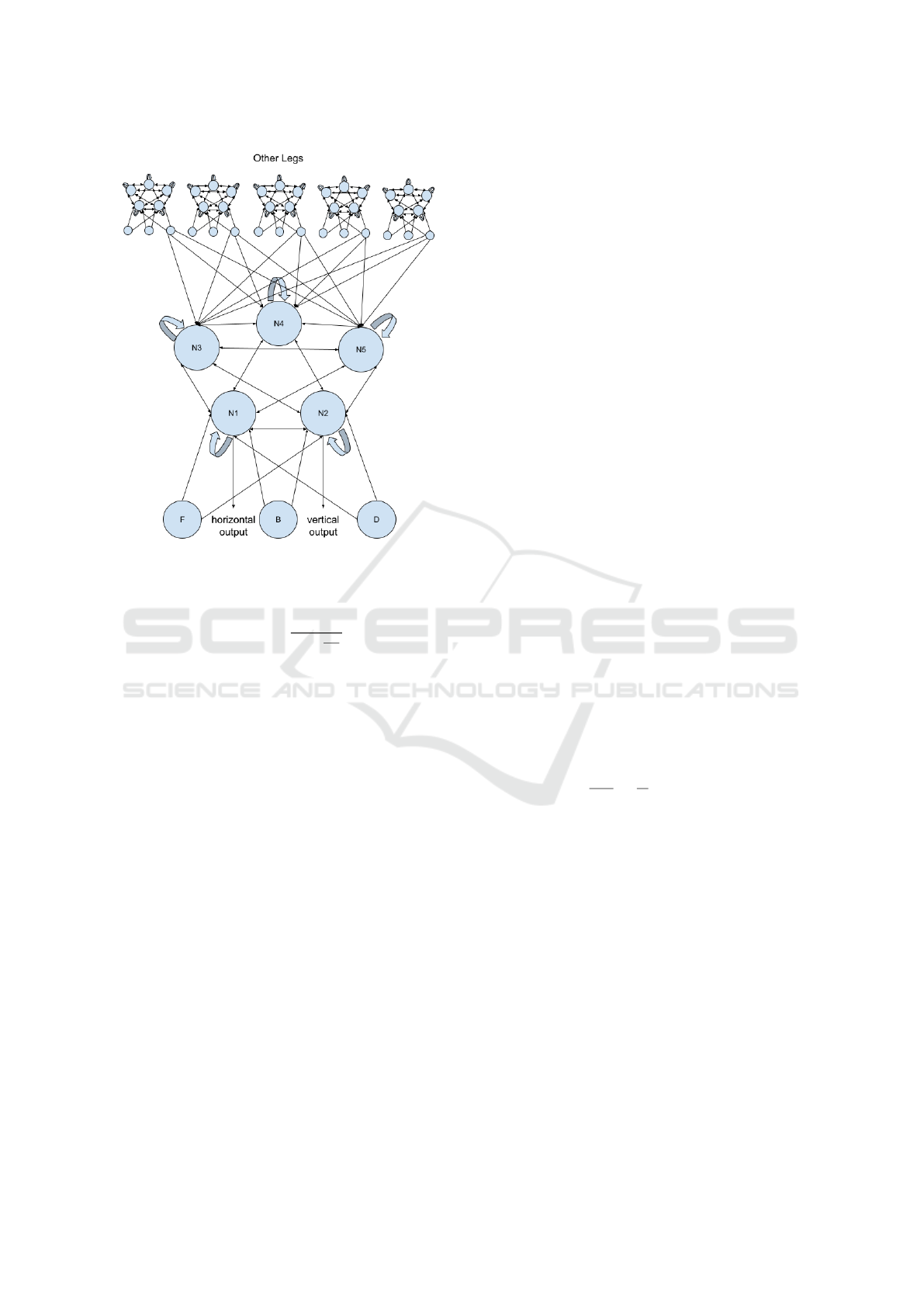
Figure 3: Neural Network Architecture (N = 5).

Furthermore, deﬁne the activation function that up-

dates the current value of neuron n as

(A) = nint



1 −e

t−A



, (5)

where nint is the ”nearest integer” function, A is the

accumulation of the neuron whose value is being up-

dated, and t and s are the thresholds of neuron n.

2.4 Simulation

As stated previously, a genetic algorithm must have a

means of determining the ﬁtness of a given solution

in a population. This is accomplished via a simula-

tion optimized for realism, efﬁciency, and simplicity.

First, we must test the hexapod for I iterations, where

I is some positive integer. This will give us a list of

coordinate positions over the I iterations of movement

for all 6 legs of the hexapod. We will then determine

the ﬁtness of the hexapod based on these coordinate

lists by calculating the hexapod’s path on a 2D ﬂat

ground. The ﬁtness is determined by how many mil-

limeters the hexapod is able to move in the forward

direction, where forward is deﬁned to be the initial

heading of the hexapod at the beginning of its test.

In secton 3.1, it is explained that momentum di-

rectly effects how much distance a servo of a leg of

the hexapod can move when provided with a pulse

width corresponding to a requested position. Momen-

tum will now be formalized for the sake of testing the

ﬁtness of a hexapod agent.

A simple version of momentum was implemented

into the simulation for each leg of the hexapod, and

which determines the distance that a leg can travel

during one iteration of the simulation. A leg has inde-

pendent components of momenum p

and p

in the

x and y directions respectively, each of which can

be any integer in the range [−3,3]. Positive p

de-

notes backward motion of the leg relative to the hexa-

pod, while negative p

denotes forward motion; sim-

ilarly, positive p

denotes upward motion relative to

the hexapod, and negative p

denotes downward mo-

tion. If the leg is moving backward and receives a

signal to move further back, its momentum will in-

crease unless it is already at maximum momentum, in

which case the momentum will remain unchanged. If

the leg is moving backward and receives a signal to

move forward, its momentum will change to −1. The

same logic of the two previous cases follows if the leg

was initially moving forward. The only way a leg can

have a momentum of 0 is if the leg receives a signal

to move to the position that it is already at.

The resulting position of a leg after receiving an

electrical signal from the controller to move to re-

quested positions x

req

and y

req

are bounded by x

max

and y

max

respectively, which are deﬁned as

∆x

max

10 ∗2

|−3

(6)

and

∆y

max

5 ∗2

|−3

, (7)

where ∆x

max

and ∆y

max

denote the maximum distance

that can be traveled in the direction of p

and p

re-

spectively. The coefﬁcients of 10 and 5 are experi-

mentally what are found to be the maximum speed of

the hexapod’s legs in the x and y directions respec-

tively in units of

25ms

m/s. In other words, the

hexapod’s legs can go at a maximum speed of approx-

imately 0.4 m/s horizontally and 0.2 m/s vertically.

Suppose the hexapod is in the nth iteration of its

testing. For each leg, the accumulation of each of

its neurons are calculated using either A

out

(l, n) or

hid

(l, n) and the new values for each neuron are cal-

culated using f (A,t) (refer to Section 3.3 for details).

The output neurons’ new values correspond to x

req

and y

req

, which are passed to the momentum algo-

rithm to calculate the leg’s momentum at iteration n.

The leg’s new position can then be calculated using

the position algorithm. Finally, all the sensors in S

are updated according to the leg’s new position.

Initially, each leg has x = 0, y = 0, p

= 0, and

= 0. For some positive number of iterations I, each

leg will follow the above procedure and return 6 lists

of I +1 positions of format (x,y) - one list per each of

the 6 legs of the hexapod. There is one more position

Coevolving Hexapod Legs to Generate Tripod Gaits

1067

than the number of iterations since the initial position

of a leg is recorded before the testing begins.

When only considering the motion of an individ-

ual leg, the forward motion at iteration n is deﬁned by

the following formula:

−x

n−1

1 + y

. (8)

This distance is only 0 if the horizontal motion of the

leg is 0 at iteration n. Therefore, even if the leg is

off of the ground (if y ̸= 0), it can still thrust itself

forward. The thrust becomes stronger if the leg is

on the ground, but this encourages the leg to lift its

leg high off the ground when repositioning after it’s

pushed all the way back, almost as though it needs

to lift its knees high because it’s walking over a thick

carpet.

For a full hexapod, the ﬁtness evaluation is much

more complex and challenging, since the hexapod can

turn, traverse a 2D plane rather than just a 1D line,

become unstable, and has many moving parts. Such a

ﬁtness evaluation is detailed as follows.

One can deﬁne a function f that will take in the

vertical height of a leg and give it a score of how much

of an effect its horizontal motion should have on the

hexapod’s motion. The function f is deﬁned as

f (h) =

(

h+a

−a, 0 ≤ h ≤ 5

0, otherwise

(9)

where

a =

√

29 −5

. (10)

This function is of the shape y =

, but intersects the

points (0, 5) and (5,0). Thus, a leg will have a maxi-

mum effect on the hexapod’s motion if h = 0 mm, and

will have no effect on the motion of the hexapod at all

if h ≥ 5 mm. This gives a similar effect as with the

individual leg, where the higher a leg lifts, the less it

will affect the motion of the hexapod, which encour-

ages the hexapod to lift its legs to a moderate height

when stepping forward.

The legs’ effectfulness scores are normalized such

that the scores of the left legs will add to 1, and the

scores of the right legs will add to 1 (unless all the

scores are 0, in which case they will remain 0). The

normalized scores can be calculated using functions

and C

deﬁned as

) =

f (h

)

f (h

) + f (h

)

(11)

and

) =

f (h

)

f (h

) + f (h

)

(12)

where i ∈{1, 3, 5} and j ∈{2, 4,6}, and if the denom-

inator of either equation 11 or 12 is 0, we set their

values to 0. Let v

...,v

be the velocities of legs

1,2 ... , 6 relative to the hexapod at the current itera-

tion; then the thrust of the left and right sides of the

hexapod is deﬁned to be

∆x

= C

, (13)

∆x

= C

. (14)

This is a weighted average of left and right leg move-

ments relative to their effectfulness. The resulting for-

ward movement of the hexapod, ∆r, is calculated as

∆r =

∆x

+ ∆x

. (15)

The yaw of the hexapod in degrees can be calculated

∆θ =

∆x

−∆x

(16)

where w is the width of the hexapod and all variables

are in identical units (see appendix for derivation).

Left turns are deﬁned to be positive degree turns and

right turns are negative.

One can account for the stability of the hexapod

to increase the realism of the simulation. Let P be

the polygon whose vertices are the tips of the hexa-

pod’s legs that are touching the ground, and let n be

the number of vertices of P. Deﬁne the hexapod to be

statically stable if its center of mass hovers above the

interior of P. Additionally, the hexapod will be par-

tially stable if its center of mass lies on the perimeter

of P. Finally, the hexapod will be unstable if its cen-

ter of mass lies outside of P entirely. If the hexapod

is statically stable, then

∆r

= ∆r. (17)

However, if the hexapod is partially stable, then

∆r

n + 6

∆r. (18)

Furthermore, if the hexapod is unstable, then

∆r

∆r. (19)

It can be seen that unstable will always have a worse

penalty than partially stable, which will always have

a worse pentalty than statically stable.

By applying these functions to the hexapod for ev-

ery iteration of its recorded movements from its test-

ing, one can get a list of ∆r’s and ∆θ’s, which can be

converted to a list of (x,y) coordinates of the hexa-

pod on a ﬂoor traversing 2D space. The ﬁtness of a

hexapod is deﬁned to be its ﬁnal x value in the path it

takes, where the hexapod begins its path at the point

(0, 0) facing in the +x direction.

ICAART 2023 - 15th International Conference on Agents and Artiﬁcial Intelligence

1068

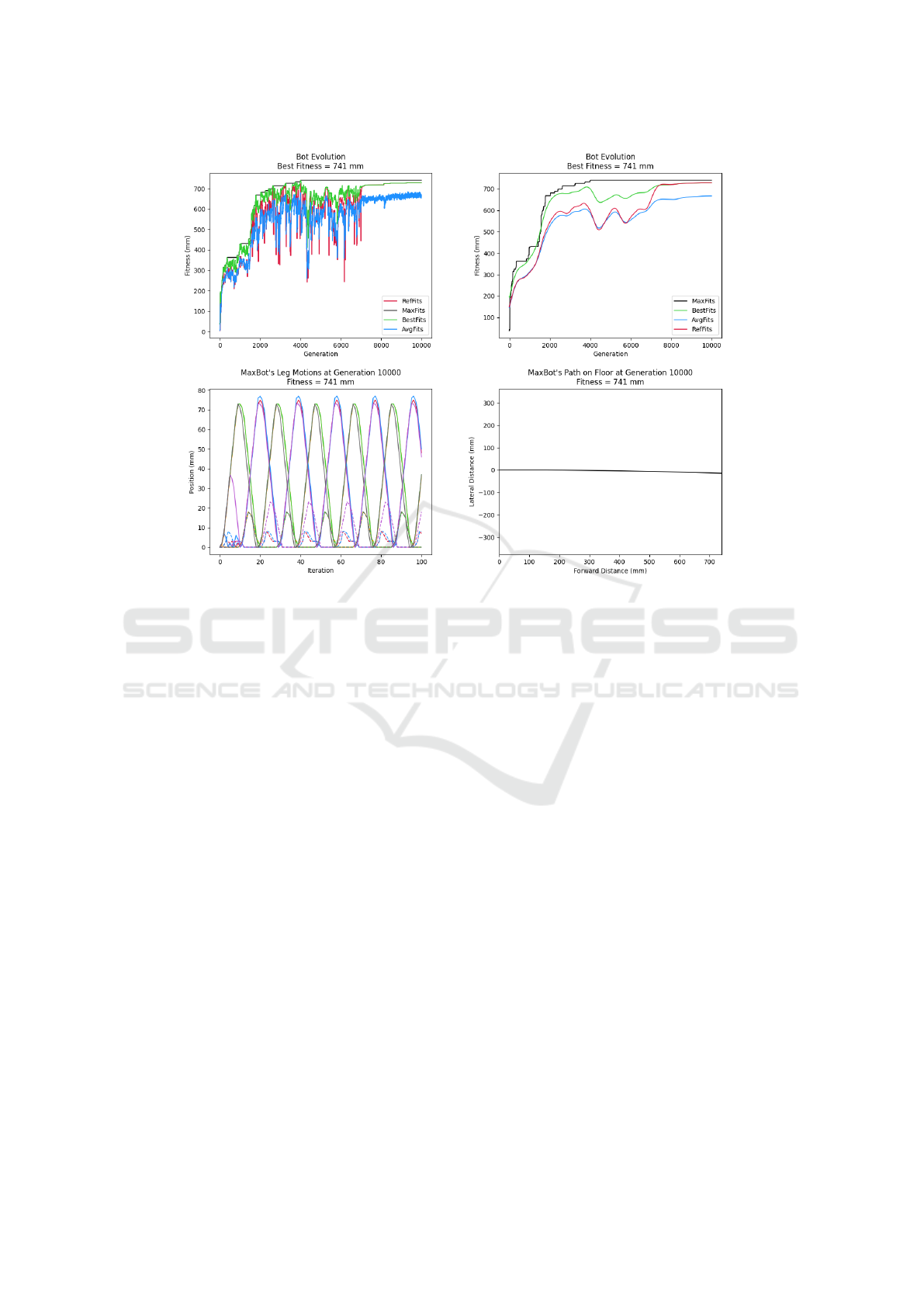
Figure 4: Run 1 (the strongest run). Top left shows learning curve raw data (MaxFits, BestFits, AvgFits, and RefFits are all

deﬁned in the text of Section 3). Top right shows data smoothed. Bottom left shows leg motions for all six legs with the solid

lines being horizontal movement (0 is full forward) and dashed lines vertical movement (0 is on the ground). Bottom right

shows the track over the ground (a horizontal line represents straight).

3 RESULTS

The results presented constitute 5 independent runs of

the genetic algorithm, where the population size is set

to 100, the number of neurons per neural network to 5,

the number of generations between reference hexapod

updates to 20, the number of iterations per hexapod

test to 100, the mutation rate to 10

−3

, and the initial

seeds for random number generation to 1 for the ﬁrst

run, 2 for the second, and so on.

Data from the highest-performing run is displayed

in Figure 4, which features four individual ﬁgures: the

ﬁrst is the original raw data of the entire evolution,

the second is that raw data smoothed out using spline

smoothing (Wahba, 1990) with λ = 10

−3

, the third is

the visualization of all six leg movements of the best

hexapod during its test, and the fourth is an overhead

view of the path of the best hexapod during its test.

For the raw and smoothed evolution graphs, for

a given generation of the graph, MaxFits represents

the highest ﬁtness seen up to that generation, BestFits

is the highest ﬁtness over all six current populations,

AvgFits is the average ﬁtness over all six current pop-

ulations, and RefFits represents the reference hexapod

ﬁtness. The smoothed evolution graph is provided to

see the general trend of the data since the raw data is

jagged and hard to read, but the raw data is impor-

tant as well since it provides unbiased data from the

evolution.

The third ﬁgure representing the leg motions of

the best hexapod of the GA run is packed with infor-

mation. If a line is solid it represents horizontal leg

motion, and if it is dashed it represents vertical leg

motion. A position of zero indicates a fully forward

leg position for solid lines or a fully down leg position

for dashed lines. The solid and dashed red lines repre-

sent the horizontal and vertical motion respectively of

the front left leg. The orange lines represent the front

right leg, green represents the middle left leg, blue

represents the middle right leg, purple represents the

back left leg, and black represents the back right leg.

The colors are conveniently in rainbow order as one

goes from the front to the back of the hexapod read-

ing legs from left to right. A tripod gait should have

the front left, middle right, and back left legs in sync,

and the front right, middle left, and back right all in

sync and doing the opposite of the ﬁrst three. Thus,

one should hope to see red, blue, and purple in sync,

Coevolving Hexapod Legs to Generate Tripod Gaits

1069

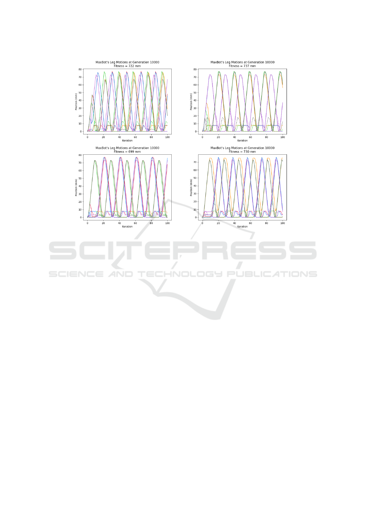
Figure 5: Leg Motions From Runs 2, 3, 4, and 5. For each graph, solid lines are horizontal movement (0 is full forward) and

dashed lines are vertical movement (0 is on the ground).

and orange, green, and black desynchronized from the

ﬁrst three and perfectly synced with one another. This

is exactly what can be seen in the leg motion graph of

Figure 4, although it may be somewhat hard to tell

since the gait was so optimized that the lines overlap

a lot, making it hard to tell which legs are in sync with

which. See Figure 5 if you aren’t convinced that the

same legs are always getting in sync with each other

to generate a tripod gait. Also, one would hope to see

that the dashed line of some color will only lift from

the zero position when the solid line of that color is

moving toward the zero position (so the leg is moving

forward). This is because if the gait is effective, the

leg should lift off the ground when it is moving for-

ward, and when the leg gets fully forward, it should

touch down to the ground, and the leg should then

proceed to move backward while remaining on the

ground. All of this behavior is exhibited in the leg

motions in Figure 4.

Finally, the fourth graph in Figure 4 represents the

path of the best hexapod during its test. Since the

ﬁtness of the hexapod is completely determined by

how far forward (the +x direction in Figure 4) it is

able to travel during its testing time, it is encouraging

to see that the hexapod’s path is straight forward with

only a slight right drift.

Figure 5 shows the leg motions of the strongest

hexapod from the 4 other GA runs. We can see using

a similar analysis to that provided for Figure 4 that all

runs achieved a strong tripod gait.

4 CONCLUSIONS

In this research, we have presented the initial work

in the development of locomotion control for a hexa-

pod robot that involves learning the values, thresh-

olds, and weights for an extensive NN system that

has nerve clusters at each leg. The nerve clusters are

made up of ﬁve neurons that are fully connected. Two

of the neurons send speciﬁc position commands to ei-

ther the up/down or back/forward servomotor of the

leg, but the remaining three neurons have no desig-

nated function. The leg controllers receive position

information from all of the other legs, but there is no

central controller. The individual leg controllers are

treated as individual agents and are coevolved to work

as a team to successfully and consistently produce a

tripod gait. To the knowledge of the authors, this is

the ﬁrst time that this has been done. In addition to

this method allowing a GA to learn the weights for

a large number of neural connections, this problem

presents an interesting task for a team of six hetero-

geneous agents to evolve to cooperate in producing

ICAART 2023 - 15th International Conference on Agents and Artiﬁcial Intelligence

1070

a reasonable gait. When comparing these results to

those of other works such as (Barfoot et al., 2006),

(Belter and Skrzypczy

nski, 2010), (Parker, 2001), and

(Parker and Rawlins, 1996), it is clear that the tech-

niques presented in this paper achieve comparable

success, as a tripod gait is consistently learned using

the same set of hyperparameters.

In future work, we intend to test the system on

the actual hexapod after adding the needed leg posi-

tion sensors and wiring connections for sensor infor-

mation between the leg controllers. In addition, we

plan to test the system by coevolving the hexapod’s

leg controllers to robustly compensate for defective,

broken, or entirely missing legs and/or controllers. It

is anticipated that such adaptive capabilities are pos-

sible with the neural network architecture presented

in this paper.

Additionally, it may also be possible to eliminate

the reference hexapod from the GA model. The GA

would then choose six individuals randomly from the

six GA’s populations and form a hexapod out of them,

and their ﬁtnesses would all be equivalent to their per-

formance as a collective hexapod. This would happen

for all the individual legs in all six populations, and

there would thus be no need for a reference hexapod,

as individuals are grouping up and getting ﬁtted dy-

namically. Such a technique would bring the results

of this paper from the coevolution of leg populations

to fully emergent hexapod gait learning. Such an evo-

lution would likely take more generations to complete

but would be an interesting result if it were achieved.

ACKNOWLEDGEMENTS

Professor Kohli of the Connecticut College Statistics

Department

REFERENCES

Barfoot, T. D., Earon, E. J., and D’Eleuterio, G. M.

(2006). Experiments in learning distributed control

for a hexapod robot. Robotics and Autonomous Sys-

tems, 54(10):864–872.

Beer, R. D. (1990). Intelligence as adaptive behavior:

An experiment in computational neuroethology. Aca-

demic Press.

Belter, D. and Skrzypczy

nski, P. (2010). A biologically in-

spired approach to feasible gait learning for a hexapod

robot.

Earon, E. J., Barfoot, T. D., and D’Eleuterio, G. M. (2000).

From the sea to the sidewalk: the evolution of hexa-

pod walking gaits by a genetic algorithm. In Inter-

national Conference on Evolvable Systems, pages 51–

60. Springer.

Gallagher, J. C., Beer, R. D., Espenschied, K. S., and Quinn,

R. D. (1996). Application of evolved locomotion con-

trollers to a hexapod robot. Robotics and Autonomous

Systems, 19(1):95–103.

Holland, J. H. (1992). Adaptation in natural and artiﬁcial

systems: an introductory analysis with applications to

biology, control, and artiﬁcial intelligence. MIT press.

Juang, C.-F., Chang, Y.-C., and Hsiao, C.-M. (2010). Evolv-

ing gaits of a hexapod robot by recurrent neural net-

works with symbiotic species-based particle swarm

optimization. IEEE Transactions on Industrial Elec-

tronics, 58(7):3110–3119.

Lee, T.-T., Liao, C.-M., and Chen, T.-K. (1988). On the sta-

bility properties of hexapod tripod gait. IEEE Journal

on Robotics and Automation, 4(4):427–434.

Lewis, M. A., Fagg, A. H., and Bekey, G. A. (1993). Ge-

netic algorithms for gait synthesis in a hexapod robot.

In Recent trends in mobile robots, pages 317–331.

World Scientiﬁc.

Parker, G. B. (2001). The incremental evolution of gaits

for hexapod robots. In Proceedings of the 3rd An-

nual Conference on Genetic and Evolutionary Com-

putation, pages 1114–1121.

Parker, G. B. and Li, Z. (2003). Evolving neural net-

works for hexapod leg controllers. In Proceed-

ings 2003 IEEE/RSJ International Conference on In-

telligent Robots and Systems (IROS 2003)(Cat. No.

03CH37453), volume 2, pages 1376–1381. IEEE.

Parker, G. B. and Rawlins, G. J. (1996). Cyclic ge-

netic algorithms for the locomotion of hexapod robots.

In Proceedings of the World Automation Congress

(WAC’96), volume 3, pages 617–622.

Potter, M. A. and Jong, K. A. D. (1994). A cooperative

coevolutionary approach to function optimization. In

International conference on parallel problem solving

from nature, pages 249–257. Springer.

Potter, M. A., Meeden, L. A., Schultz, A. C., et al. (2001).

Heterogeneity in the coevolved behaviors of mobile

robots: The emergence of specialists. In International

joint conference on artiﬁcial intelligence, volume 17,

pages 1337–1343. Citeseer.

Spencer, G. F. (1993). Automatic generation of programs

for crawling and walking. In Proceedings of the

5th International Conference on Genetic Algorithms,

page 654.

Vice, J., Sukthankar, G., and Douglas, P. K. (2022). Lever-

aging evolutionary algorithms for feasible hexapod

locomotion across uneven terrain. arXiv preprint

arXiv:2203.15948.

Wahba, G. (1990). Spline models for observational data.

SIAM.

Wiegand, R. P., Liles, W. C., De Jong, K. A., et al. (2001).

An empirical analysis of collaboration methods in

cooperative coevolutionary algorithms. In Proceed-

ings of the genetic and evolutionary computation con-

ference (GECCO), volume 2611, pages 1235–1245.

Morgan Kaufmann San Francisco.

Coevolving Hexapod Legs to Generate Tripod Gaits

1071