FlexPooling with Simple Auxiliary Classiﬁers in Deep Networks

Muhammad Ali

, Omar Alsuwaidi and Salman Khan

Department of Computer Vision, Mohamed bin Zayed University of Artiﬁcial Intelligence (MBZUAI), Abu Dhabi, U.A.E.

Keywords:

Global Average Pool, Flexpool, Multiscale, Regularized Flexpool, Simple Auxiliary Classiﬁer(SAC).

Abstract:

In Computer Vision, the basic pipeline of most convolutional neural networks (CNNs) consists of multiple

feature extraction processing layers, wherein the input signal is downsampled into a lower resolution in each

subsequent layer. This downsampling process is commonly referred to as pooling, an essential operation

in CNNs. It improves the model’s robustness against variances in transformation, reduces the number of

trainable parameters, increases the receptive ﬁeld size, and reduces computation time. Since pooling is a lossy

process yet crucial in inferring high-level information from low-level information, we must ensure that each

subsequent layer perpetuates the most prominent information from previous activations to aid the network’s

discriminability. The standard way to apply this process is to use dense pooling (max or average) or strided

convolutional kernels. In this paper, we propose a simple yet effective adaptive pooling method, referred to

as FlexPooling, which generalizes the concept of average pooling by learning a weighted average pooling

over the activations jointly with the rest of the network. Moreover, attaching the CNN with Simple Auxiliary

Classiﬁers (SAC) further demonstrates the superiority of our method as compared to the standard methods.

Finally, we show that our simple approach consistently outperforms baseline networks on multiple popular

datasets in image classiﬁcation, giving us around a 1-3% increase in accuracy.

1 INTRODUCTION

In the current Computer Vision community, the vast

majority of image label learning techniques rely on

the hard classiﬁcation of samples in order to learn

a function mapping between the images and their

corresponding classes. Usually, under a supervised

training setting, class-label learning involves using

cross-entropy and binary cross-entropy loss functions

for multiclass and binary class classiﬁcation, respec-

tively. The choice for the hypothesis class to learn the

label function mapping is most often parameterized

as a convolutional neural network (CNN) with multi-

ple processing and downsampling layers. CNNs are

very suitable for such a task as they mimic our natural

ability to perceive images by dividing an image into

many small sub-images and processing them locally

for feature extraction, one by one. They also utilize

parameter sharing via learned convolutional kernels

based on the assumption that learning a meaningful

pattern in one part of the image may also be help-

ful in another part of the image, and that is especially

true in the early stages of the CNN, where the features

learned by the convolutional kernels tend to be less

https://orcid.org/0000-0001-9320-2282

https://orcid.org/0000-0002-9502-1749

abstract and more generalizable. Moreover, thanks to

their intrinsic design, they can gradually reduce the

dimension of the input, allowing for faster processing,

reduction in the number of parameters, and increased

receptive ﬁeld size, which in turn allows the model

to learn high-level information from low-level ones.

All these properties have made CNNs very robust and

efﬁcient models when dealing with image processing.

Another building block of almost all convolutional

neural networks (CNNs) is a crucial technique known

as pooling, a process that signiﬁcantly downscales the

incoming image by preserving a small portion of the

feature map, which resembles the most important pix-

els for the task solution. A usual pipeline of a CNN

is composed of multiple stages, where each stage in-

volves a series of feature extraction (convolutional)

layers, followed by a pooling layer, where the image

gets downscaled further in each consecutive stage.

Pooling allows the CNN model to be invariant to

tiny distortions and further perturbations in the image.

It also dramatically enlarges the receptive ﬁeld be-

tween intermediate and output nodes while lowering

the computational cost and parameter count, similar

to what a convolutional kernel does but more ampli-

ﬁed (Papineni et al., 2001). Out of the possible pool-

ing methods, Average or mean pooling and Max pool-

Ali, M., Alsuwaidi, O. and Khan, S.

FlexPooling with Simple Auxiliary Classiﬁers in Deep Networks.

DOI: 10.5220/0011894400003417

In Proceedings of the 18th International Joint Conference on Computer Vision, Imaging and Computer Graphics Theory and Applications (VISIGRAPP 2023) - Volume 4: VISAPP, pages

497-505

ISBN: 978-989-758-634-7; ISSN: 2184-4321

 2023 by SCITEPRESS – Science and Technology Publications, Lda. Under CC license (CC BY-NC-ND 4.0)

497

ing are the two most frequently used pooling tech-

niques in various CNN architectures like VGG (Karen

Simonyan & Andrew Zisserman, 2018), ResNet (He

et al., ), and GoogLeNet (Szegedy et al., 2015).

Despite their popularity and widespread use, av-

erage pooling and max pooling possess serious draw-

backs and model limitations. For one, despite the en-

tire ensemble of parameters in a CNN being trained

jointly from end to end, the average and max pool-

ing layers, by deﬁnition, are unlearnable and hence do

not adapt well to seen data during training nor gen-

eralize effectively to unseen data (Gholamalinezhad

and Khosravi, 2020a). Furthermore, since pooling is

a lossy process that discards some information from

the incoming data, we need to ensure that our pooling

process extracts the most prominent and relevant in-

formation for the end task solution. However, average

and max pooling both rely on an a priori assumptions:

the mean of locally neighboring pixels is a good rep-

resentation of the region, and the maximum response

from a group of neighboring pixels is the most rele-

vant representation in that region, respectively. While

these assumptions have some theoretical justiﬁcation

and can be worked around via learnable convolutional

kernels, they can easily hinder the network’s ability to

learn efﬁciently and serve as a bottleneck because of

their incompatibility in adapting to activations due to

lack of learnability. More recent CNN designs, like

ResNets, frequently apply convolutions with strides

greater than one as a replacement for pooling layers.

However, strided convolutions come with their own

disadvantages and fail to act as an actual pooling pro-

cess. Conversely to traditional pooling layers, they no

longer treat and pool each feature map independently;

instead, they aggregate all the feature maps channel-

wise to get the resulting output activation. Lacking

the ability to pool each feature map independently

goes against the inherent design of CNNs, where the

generation of each feature map in a stack of feature

maps is the result of a single convolutional kernel that

is independent of other convolutional kernels which

generated the rest of the feature maps in the same

stack. Hence, each feature map represents a unique

distribution of locally extracted features that might be

similar but independent of the rest of the feature maps

in the same stack. That is why it is of utmost impor-

tance to treat and pool each feature map individually

in order to be able to extract and perpetuate the most

meaningful compact representation during the lossy

process of pooling.

However, in recent years and with the advance-

ments of CNN architectures, the most common use

case of downsampling via pooling has been the use

of Global Average Pooling, which holistically aver-

ages the feature maps individually across the height

and width dimensions in the last convolutional stage

before feeding the outcome into the projection head

in order to make the class prediction (Ren et al.,

2015). Global average pooling offers multiple advan-

tages over the traditional way of using fully connected

layers. It reduces the number of trainable parameters,

also enforcing correspondences between feature maps

and classes. Therefore, allowing us to interpret the ﬁ-

nal processed feature maps as class conﬁdence maps.

Despite these signiﬁcant beneﬁts of using global av-

erage pooling over fully connected layers, they still

suffer from the same limitations as the standard av-

erage pooling that were discussed earlier in this pa-

per, mainly incompatibility in adapting to activations

due to lack of learnability, which can hurt the model’s

ability to generalize to unseen data.

In this work, we primarily focus on improving this

vital yet often overlooked process of feature map to

class correspondence via global pooling. We aim to

replace the global average pooling layer by substi-

tuting it with a more robust ﬂexible pooling layer,

named FlexPool, that is trainable jointly with the

network in an end-to-end fashion and is fully dif-

ferentiable. FlexPool aims to learn the best set of

weights in a weighted average for each feature map in

the last stage of convolutions, allowing the model to

learn the appropriate correspondences between fea-

ture maps and categories. Having the ability to learn

a weighted average global pooling over the feature

maps with the rest of the network, FlexPool is an ef-

fortless yet efﬁcient adaptive pooling technique that

generalizes the idea of global average pooling. Ad-

ditionally, attaching the CNN with Simple Auxiliary

Classiﬁer (SAC) heads along different convolutional

stages further demonstrates our method’s superiority

over standard global average pooling.

We demonstrate that substituting FlexPooling as

the global pooling layer of choice improves perfor-

mance on the different datasets using different ResNet

sizes. With the introduction of this simple but effec-

tive technique, we propose using it with any existing

state-of-the-art CNN to get improved results easily. In

order to further explain the concept sequentially, we

organized the rest of the paper as follows; Section 2

reviewed the related work done on pooling layers. In

Section 3, we present our suggested model and dictate

its formulation, explaining the effects of FlexPooling

and its variants. We describe the experiments and

analyze the outcomes of those experiments in detail

in Section 4 using different benchmark datasets and

models. Finally, Section 5 concludes with a summary

of our work.

VISAPP 2023 - 18th International Conference on Computer Vision Theory and Applications

498

2 MATERIALS AND METHODS

Among the two most popular pooling techniques (av-

erage and max pooling), max pooling tends to out-

perform average pooling in terms of discriminability

in most CNN architectures and tasks, especially for

features with low activation intensities, as studied by

(Boureau et al., 2010a) when examining the different

pooling techniques. Max pooling seeks to preserve

the most important details because it is crucial for

the network’s ability to discriminate (Boureau et al.,

2010b). However, because only one node is chosen in

each local neighborhood, this can cause the gradient

ﬂow to experience a disruption in its gradient mag-

nitudes in connections branching out from that node

during the backward pass of the CNN. Max pooling

also produces relatively sparse results when down-

scaling images (Gulcehre et al., 2013). Moreover, the

fact that the appropriate choice of pooling relies upon

the CNN structure and dataset distribution is another

drawback of traditional pooling layers, which requires

the practitioner to perform extensive empirical testing

to determine the appropriate pooling technique for the

speciﬁc task solution.

Since the two most commonly used methods for

pooling both have their own advantages and limi-

tations, one might suspect that the best way to ex-

tract meaningful information during pooling may fall

somewhere between the two methods of average and

maximum pooling. Previous research on pooling

techniques has focused on using unusual pooling ra-

tios or altering the receptive ﬁeld size of the pooled

region.

Researchers like (Ionescu et al., 2015) offered

a strategic approach to make it possible to include

deeper networks with higher-order pooling layers.

Performing inter-channel max pooling is advised by

Maxout (Goodfellow et al., 2013), while a fractional

downscaling ratio is used in fractional pooling (Gho-

lamalinezhad and Khosravi, 2020b), which results in

a more steady size reduction. Low-pass ﬁltering was

implemented by (Rippel et al., 2015) to downsample

feature maps in spectral space. As details are primar-

ily concentrated in higher frequencies, this smoothes

the input rather than maintaining them. Researchers

also worked on various receptive ﬁeld sizes of pooled

pixels(Rippel et al., 2015). Ionescu et al. offer a strat-

egy that makes it possible to include deeper networks

with higher-order pooling layers, As details are pri-

marily focused on higher frequencies, this smoothens

the input rather than maintaining them (Saeedan et al.,

2018) through learnable pooling layers, recent re-

search has sought to maintain the most discrimina-

tive parts of the data/activations and eliminate the re-

dundant ones. There have been several attempts to

combine max and average pooling(Gholamalinezhad

and Khosravi, 2020b); nonetheless, none truly suc-

cessfully harnessed the advantages in both (Gholama-

linezhad and Khosravi, 2020b). Other pooling tech-

niques included scaling according to the input size

(He et al., 2014), enabling CNNs to handle a range

of image sizes.

In study (Saeedan et al., 2018), researchers pro-

posed a method to preserve the subtle elements within

an input image that are essential in representing an

accurate visual impression. Its purpose was to retain

the reﬁned details typically lost by the average pool-

ing and have it improved along the network in the

learning path, thereupon helping us to get the relevant

missing information. This approach motivates this

work in attempting to preserve the ﬁne pixel-speciﬁc

details and avoid losing any information as much as

possible; thus, we replace the existing standard aver-

age pooling with our novel FlexPooling layer.

3 METHODOLOGY

3.1 FlexPool

FlexPooling, is a revolutionary trainable pooling strat-

egy which is inspired by (Allen et al., 2019) and (Sim-

sek et al., 2021), who found that overparameterized

neural networks converge faster and generalize better

to various datasets. It makes average pooling more

general by learning a weighted average pooling over

the latent feature activations of the network at the

same time. FlexPool improves feature map to class

correspondence by using parameters trained jointly

end-to-end We Replace FlexPooling’s global average

pooling layer with one that is more robust, ﬂexible,

and trainable from beginning to end. In the last step

of convolutions, FlexPool learns the best weights for

a weighted average sum for each feature map. This

helps the model understand how feature maps and cat-

egories are linked. This basic version is described in

Figure 1.

Our methodology consists of two main parts;

ﬁrstly, we introduce the concept of the trainable pool-

ing layer, FlexPooling, which aids in the convergence

of our objective function. Secondly, we augment the

CNN implementation with SACs to further demon-

strate the effectiveness of our FlexPooling technique

compared to traditional approaches like global av-

erage pooling. SACs do not require any additional

processing units like dense or convolutional layers;

instead, they immediately take the feature map rep-

resentation (block) at any particular stage, then col-

FlexPooling with Simple Auxiliary Classiﬁers in Deep Networks

499

lapse it into a ﬂattened vector through a global pool-

ing approach. The detailed description of two ap-

proaches are summarized in Figure 1 and Figure 3,

respectively. First, we present and detail FlexPool-

ing, a novel trainable pooling technique inspired by

the works and ﬁndings of (Allen et al., 2019), (Sim-

sek et al., 2021), whom all concluded that overparam-

eterized neural networks achieve easier convergence

and generalize better to different datasets. It serves

as a simple yet effective adaptive pooling method that

generalizes the concept of average pooling by learn-

ing a weighted average pooling over the network’s

latent feature activations jointly with the rest of the

network. FlexPool primarily focuses on improving

the vital yet often overlooked process of feature map

to class correspondence via a global pooling opera-

tion. In FlexPooling, replace the global average pool-

ing layer with a more robust and ﬂexible pooling layer

that is trainable jointly with the rest of the network

in an end-to-end fashion and is fully differentiable.

FlexPool aims to learn the best set of weights in a

weighted average sum for each feature map in the last

stage of convolutions, allowing the model to better

learn the appropriate correspondences between fea-

ture maps and categories. For any given input image

X that is passed through the convolutional operation

for feature extraction, the resulting feature map is a

processed and downsampled version of the input im-

age. As we process deeper through the CNN, the fea-

ture map representation of the input image continues

to shrink along the height and width dimensions (size)

while enlarging along the channel dimension (depth).

During the last stage of processing, a global average

pooling layer is applied to each individual feature map

resulting in a single output for each feature map as a

ﬂattened vector. This global pooling helps the CNN

establish a correspondence between feature maps and

classes as class conﬁdence maps. Finally, the ﬂat-

tened vector is sent to the network’s project head,

which usually consists of a series of non-linearly ac-

tivated dense layers, before being sent to the softmax

function to generate class predictions. This setup is

the most adopted setup when using CNNs. The re-

sulting size of a feature map after being processed by

a convolution operation is given by the following (Ng,

2020):

(N − K + 2P)

+ 1 (1)

where N is the feature map’s input volume, K is the

convolution’s kernel size, P is the number of padding,

and S represents the stride of the kernel.

In addition to the traditional approach, during the

last stage of processing, we replicate the shape of the

ﬁnal feature maps to initialize our FlexPooling block

such that it matches the ﬁnal stage’s block shape. The

FlexPooling block consists of trainable parameters,

each initialized to resemble the value of the global

average pooling layer. Hence, every value in the Flex-

Pooling block initially is set to

height×width

. After-

ward, the dot product is taken between the FlexPool-

ing block and the ﬁnal stage’s processed block to ob-

tain a weighted block. Finally, we sum across the

size of the weighted block, yielding a weighted av-

erage output for each feature map. The objective is

to have these values be trainable parameters in such

a manner that it aids in the model learning process

during training. However, nothing guarantees that the

FlexPool blocks’ parameters remain as weighted av-

erage values. In fact, due to the stochasticity and the

noise in the training process, it very well might be the

case that some of the parameters can take on negative

values, thus, no longer representing a weighted aver-

age. To tackle this issue, we propose to regularize the

FlexPooling parameters



f p



by introducing a reg-

ularization term R (FlexPool) in such a way that en-

forces a weighted average when summing the param-

eter values across the size of the FlexPooling block.

This parameter regularization can be accomplished in

a couple of ways. In our experiments, we utilize the

Mean Square Error (MSE) difference to enforce the

desired behavior on the FlexPool parameters:

R(FlexPool) =

∑

k=1

∑

i=1

∑

j=1

f p

i, j,k

− 1

(2)

where N is the FlexPool’s volume size, C is the num-

ber of channels in the FlexPool block, and w

f p

i, j,k

is the

weight in the i

row, j

column of the k

channel in

the FlexPool block.

3.2 FlexPool with SAC

Here our suggested network takes feature maps from

early stages and compress them into linear representa-

tion via FlexPooling, where no convolutional process-

ing is involved,yet we downsample the feature maps

into single pixel representation.

Compared to basic FlexPooling, here we adopt

FlexPooling with the attachment of Simple Auxiliary

Classiﬁers(SAC) onto the CNN to further observe the

effects of pooling feature maps at different stages on

accuracy. The loss values at each stage of the CNN

are aggregated to obtain a weighted average loss. Par-

ticular weights λ1, λ2, and λ3, provided as hyper-

parameters, are assigned to each loss function that

emerged from each stage of the CNN. We note that

the following condition of the loss weights must hold

VISAPP 2023 - 18th International Conference on Computer Vision Theory and Applications

500

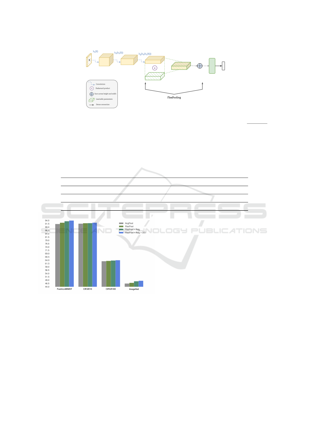
Figure 1: Proposed Method: After passing the image X through a series convolutional layers in ResNet20 we initialize a

FlexPooling block composed of learnable parameters that matches the shape of the feature maps in the last stage. Those

parameters are initialized to resemble global average pooling layer (the initialized value for each parameter is

height×width

Finally, we take the dot product of the two blocks and sum across the height and width dimensions, resulting in the ﬁnal

ﬂattened layer before the projection head is applied, yielding the class predictions in gray.

Table 1: FlexPooling: Performance comparison on benchmark datasets, including ImageNet, CIFAR10, Fashion-MNIST,

and CIFAR100. ResNet20 is used as the baseline of this experiment, though any model can be used. It is apparent across all

datasets that adopting FlexPool yields optimal results as compared to the standard average pooling. An increased accuracy

trend emerges when moving across the columns of each row in the table, demonstrating the consistency and effectiveness of

FlexPooling.

Dataset Methods AvgPool FlexPool FlexPool + Reg FlexPool + Reg + Dropout

CFAR10 91.63 91.91 91.87 92.32

Fashion-MNIST 91.38 92.35 93.48 93.98

CFAR100 66.18 66.50 66.73 68.30

ImageNet 46.50 47.03 48.11 48.55

Figure 2: FlexPooling performance on different benchmark

datasets. As given in Table 1, these plots show consistent

improvement in accuracy with the introduction of FlexPool-

ing and its variants.

to achieve stable learning: λ

< λ

. The ﬁnal

weighted average loss is given by:

Loss = λ

L (h

(x), y) + λ

L (h

(x)), y)

+ λ

L (h

(x))), y) (3)

where the loss function L used is the categorical cross-

entropy loss(Zhang and Sabuncu, 2018), given by:

L((h (x), y)) = −

∑

c=1

o,c

log(h

o,c

) (4)

Where M is the number of classes, h is predicted

probability observation of class c, and y is true label

assigned to class c. In our experiments, the weights

corresponding to the loss functions from each stage

were set to λ

= 0.1, λ

= 0.2 and λ

= 0.7. After

the aggregate loss is computed from weighted cross

entropy losses at different stages, we back propa-

gate the loss through the entire network to update

the model parameters, including FlexPool’s parame-

ters. We evaluate our approach on various benchmark

datasets in image classiﬁcation, to demonstrate its ef-

fectiveness.

4 RESULTS AND DISCUSSIONS

We evaluate our proposed classiﬁer with Flex-

Pooling, on several datasets including, Tiny Ima-

geNet(Le and Yang, 2016), CFAR100(Krizhevsky,

2009), and also very small scale datasets in-

cluding CFAR10(Krizhevsky, 2009) and FashionM-

NIST(Xiao et al., 2017) and compare it with stan-

dard classiﬁer using average pooling. We conduct ex-

tensive evaluation study to evaluate the effect of dif-

ferent components on the performance of our model.

We use accuracy as the evaluation metric for perfor-

FlexPooling with Simple Auxiliary Classiﬁers in Deep Networks

501

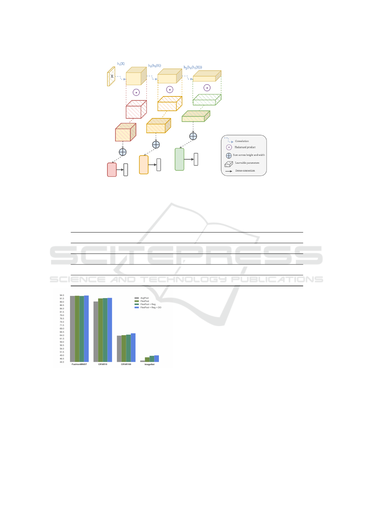
Figure 3: FlexPooling with SACs approach. The cross-entropy loss is calculated for each class prediction (in gray) after

every FlexPooling block and is taken as a weighted sum to obtain the ﬁnal loss. The loss values obtained from different stages

of the CNN aid the network in learning more abstract concepts by boosting the gradient signal throughout the entire network.

Table 2: FlexPooling wih SAC’s: Performance comparison on benchmark datasets, including ImageNet, CIFAR10, Fashion-

MNIST, and CIFAR100. ResNet20 is used as the baseline of this experiment, though any model can be used. Signiﬁcant

improvement is exhibited in all datasets when going from AvgPool to FlexPool. While the best improvement is shown in

ImageNet, a consistent improvement in accuracy is also demonstrated in the other datasets.

Datasets/Methods AvgPool FlexPool FlexPool + Reg FlexPool + Reg + Dropout

CIFAR10 89.31% 91.61% 91.86% 92.03%

Fashion-MNIST 93.55% 93.65% 93.48% 93.84%

CIFAR100 63.79% 64.12% 64.53% 65.57%

ImageNet 45.13% 47.55% 48.64% 49.01%

Figure 4: FlexPooling with SAC performance on different

benchmark datasets. As given in Table 2, these plots show

further consistent improvement in accuracy with the intro-

duction of FlexPooling and its variants.

mance evaluation of our approach. We conduct ex-

periments in two settings, including with FlexPooling

only, FlexPooling with auxiliary classiﬁers. In each

setting we evaluate different combinations: FlexPool

only, FlexPool with regularization and FlexPool with

regularization and droput.

4.1 Experimental Setup and

Implementation Details

We take the input image of size 32x32 in the case

of tiny ImageNet and pass it through the convolu-

tional blocks of ResNet20 in our case, we may use

any other network. We apply our method in two set-

tings : in the single classiﬁer settings an image x is

pass through different convolutional blocks and we

apply FlexPooling at the end before feeding it to the

linear classiﬁer and compute the relevant cross en-

tropy loss. For the FlexPool using SAC our model

takes the feature maps from early stages prematurely

and compresses them into a linear representation via

FlexPooling, where no convolutional processing is in-

volved, only completely downsampling the feature

maps into singlepixel representation. We repeat this

procedure after each available convolutional blocks

and then take the weighted sum of these which give

us our ﬁnal loss which we use to train our model. For

our case we designate the weights of the loss as λ1, λ2

and λ3 whose values after cross validation we choose

VISAPP 2023 - 18th International Conference on Computer Vision Theory and Applications

502

as 0.1, 0.2 and 0.7 respectively. Learning rate use is

0.1 and we use one cycle learning rate.

4.2 Training Details

For the case of FlexPooling method we train our mod-

els for 100 epochs with batch size 1000 for one A100

GPU. For the case of super classing we train it two

steps, in the ﬁrst stage we train for 10 epochs and then

in the next step we train it for 100 epochs. We use the

ADAM(Kingma and Lei Ba, 2015) optimizer with an

initial learning rate 0.1. We also use augmentation of

random ﬂipping, scaling to improve the generaliza-

tion ability of our model.

4.3 Main Results

As shown in Table 1, we test our model on several low

scale and medium scale bench mark datasets. Where

Backbone use in our case is ResNet20 we may use any

other backbone. The Avg pool shows the accuracy

we obtain with standard average pooling while Flex-

Pool indicates the accuracy obtained after the Flex-

Pooling. Further, results with regularization as well

as with addition of drop out are also given. We can

see in the Table 1 that we get an overall increase of

1.5 to 2% across all range of datasets when we ap-

ply FlexPooling method in single classiﬁer settings.

Further we also give the results for the case when

we apply FlexPooling with multiscaling i.e we take

varied scale outputs after each convolutional blocks

and use FlexPooling individually after each block and

then average these multiscaled losses to get the ﬁnal

weighted loss. The results for this approach give us

clear increase of 1 - 3 % increase across the range of

all datasets.

4.4 Ablation Study

To further analyze the ability of our proposed method,

we conduct extensive ablation studies on the several

datasets to explore the effects of our components. We

use the ofﬁcial training and validation split and accu-

mulate the evaluation results over the whole training

set. The ablation study results are shown in Table 1,

Table 2 and Table 3. Our baseline model use aver-

age pooling, whereas we introduce the FlexPool and

FlexPool with SAC, replacing standard average pool-

ing to see the effects. Below we discuss the different

ablation studies we perform during the course of our

experiments to validate our method.

4.4.1 Effect of FlexPooling

Initially we apply the FlexPooling after the ﬁnal con-

volutional block before feeding the features maps to

the ﬁnal projection layer. Results in Table 1 conﬁrm

that FlexPooling improves the performance of our

model for all datsets discussed. We get the highest

increase for the case of ImageNet benchmark which

give us almost 0.5% increase without any regulariza-

tion and dropout. We then apply regularization for im-

proving the generalization and we see further 1% in-

crease which give us 48.11 accuracy compared

to the average pooling which give us 46.5 accuracy.

We see that adding 25 % dropout increases the ac-

curacy to 48.55. Similarly for the case of CFAR100

we get increase of 0.3 % without regularization to

1.8% increase with regularization and dropout. We

see similar trends for the case of other datasets given

in Table 1.

For these settings we get the best results for the

case of Tiny ImageNet which improves the result

by almost 2 %. The FlexPool with regularization

and using drop out of 0.25 outperforms in accuracy

as it is able to learn jointly with entrire network,

thus enhance its ability to exract more meaningful

feature map representations that help with model’s

generalizability and discriminability.

4.4.2 Effect of FlexPooling Using SAC

We further extend our idea of FlexPooling such that

instead of applying it at the end of last convolutional

block before the linear projection layer, we take the

outputs at different depths of model and apply the

FlexPooling at these depths and then we use Cross

Entropy loss (CEL) to contribute in the total loss

which is comprised of average of weighted sum of

all these losses.

Table 2 conﬁrms the improved accuracy obtain by

multiscale FlexPooling while using simple auxiliary

classiﬁers(SAC). Here network takes feature maps

from early stages and compress them into linear rep-

resentation via FlexPooling, where no convolutional

processing is involved,yet we downsample the feature

maps into single pixel representation. also sustain the

increase but it give us overall increase of 0.75 % to

2.3% increase over the range of all the datasets.

Results in Table 2 conﬁrm that adding FlexPool-

ing stages helps improve the performance of our

model in different ranges. We get the best increase

for the case of Tiny ImageNet dataset which give us

almost 2.3% increase without any regularization and

dropout. We then apply regularization for improv-

ing the generalization and we see further 1.10% in-

FlexPooling with Simple Auxiliary Classiﬁers in Deep Networks

503

crease which give us 48.64 accuracy compared to the

average pooling which give us 46.5 accuracy. We see

that adding 0.25 % dropout and regularization weights

give us nearly 3.5% improvement. Similarly for the

case of CFAR100 we get increase of 0.75 % with-

out regularization to 1.1% increase with regulariza-

tion and dropout. We see similar trends for the case

of other datasets given in Table 1. For these settings

we get the best results for the case of Tiny ImageNet

which improves the result by almost 3.5 %. The con-

sistent improvement across various datasets show the

stability of the method.

5 CONCLUSIONS

In this paper, we present FlexPooling approach with

and without simple auxiliary classiﬁer(SAC). Flex-

Pooling with SAC is a straightforward but efﬁcient

adaptive pooling technique that learns weighted av-

erage pooling over activations together with the rest

of the network, thus generalizing the idea of aver-

age pooling with consistent improved performance.

In our approach, we make sure that each successive

layer repeats the most salient information from the

prior activations because pooling is a lossy opera-

tion but essential in separating high-level informa-

tion from low-level information. This improves the

network’s discriminability. Secondly for FlexPooling

with SAC our suggested network takes feature maps

from early stages and compress them into linear rep-

resentation via FlexPooling, where no convolutional

processing is involved, yet we downsample the fea-

ture maps into single pixel representation. The loss

values obtained from early stages of the CNN aid the

network in learning more abstract concepts by boost-

ing the gradient signal throughout the entire network.

Our approach learns jointly with the entire network

end to end, enhancing its ability to adapt and ex-

tract more meaningful feature, map representations

that help with the model’s discriminability and gener-

alizability We validate this claim by extensive exper-

iments in single-classiﬁers as well as multi-classiﬁer

settings. We obtain the stable, increasing accuracy

trend in both settings from the average pool to ﬂex

pool. We show further improvement in accuracy

when each of above mentioned settings are tested with

three different ablation studies, including FlexPool,

FlexPool with regularization and FlexPool with regu-

larization and dropout. Overall, FlexPool with(SAC)

settings attain higher accuracies on average compared

to a single classiﬁer thanks to improved gradient sig-

nal throughout the CNN. Finally, we demonstrate that

our technique consistently outperforms baseline net-

works in image classiﬁcation across a variety of pop-

ular datasets, resulting in accuracy gains of 1-3%.

REFERENCES

Allen, Z., Zeyuan, L., Yuanzhi, L., and Yingyu (2019).

Learning and generalization in overparameterized

neural networks, going beyond two layers. in ad-

vances in neural information processing systems.

Boureau, Y.-L., Ponce, J., Fr, J. P., and Lecun, Y. (2010a).

A Theoretical Analysis of Feature Pooling in Visual

Recognition.

Boureau, Y.-L., Ponce, J., and LeCun, Y. (2010b). A the-

oretical analysis of feature pooling in visual recogni-

tion. In Proceedings of the 27th International Confer-

ence on International Conference on Machine Learn-

ing, ICML’10, page 111–118, Madison, WI, USA.

Omnipress.

Gholamalinezhad, H. and Khosravi, H. (2020a). Pooling

methods in deep neural networks, a review. arXiv

preprint arXiv:2009.07485.

Gholamalinezhad, H. and Khosravi, H. (2020b). Pooling

Methods in Deep Neural Networks, a Review.

Goodfellow, I. J., Warde-Farley, D., Mirza, M., Courville,

A., and Bengio, Y. (2013). Maxout Networks. 30th In-

ternational Conference on Machine Learning, ICML

2013, (PART 3):2356–2364.

Gulcehre, C., Cho, K., Pascanu, R., and Bengio, Y. (2013).

Learned-Norm Pooling for Deep Feedforward and Re-

current Neural Networks.

He, K., Zhang, X., Ren, S., and Sun, J. Deep Residual

Learning for Image Recognition.

He, K., Zhang, X., Ren, S., and Sun, J. (2014). Spatial Pyra-

mid Pooling in Deep Convolutional Networks for Vi-

sual Recognition. Lecture Notes in Computer Science

(including subseries Lecture Notes in Artiﬁcial Intel-

ligence and Lecture Notes in Bioinformatics), 8691

LNCS(PART 3):346–361.

Ionescu, C., Vantzos, O., and Sminchisescu, C. (2015).

Training deep networks with structured lay-

ers by matrix backpropagation. arXiv preprint

arXiv:1509.07838.

Karen Simonyan & Andrew Zisserman (2018). very deep

convolutional networks for large-scale image recogni-

tion. American Journal of Health-System Pharmacy,

75(6):398–406.

Kingma, D. P. and Lei Ba, J. (2015). Adam: A method for

stochastic optimization. ICLR.

Krizhevsky, A. (2009). Learning multiple layers of features

from tiny images. arXiv.

Le, Y. and Yang, X. (2016). Tiny imagenet visual recogni-

tion challenge. arXiv.

Ng, A. (2020). Cs 230 - convolutional neural networks

cheatsheet. Stanford CS230.

Papineni, K., Roukos, S., Ward, T., and Zhu, W.-J. (2001).

BLEU. Proceedings of the 40th Annual Meeting on

Association for Computational Linguistics - ACL ’02,

page 311.

VISAPP 2023 - 18th International Conference on Computer Vision Theory and Applications

504

Ren, S., He, K., Girshick, R., and Sun, J. (2015). Faster

R-CNN: Towards Real-Time Object Detection with

Region Proposal Networks. undeﬁned, 39(6):1137–

1149.

Rippel, O., Snoek, J., and Adams, R. P. (2015). Spectral

Representations for Convolutional Neural Networks.

Advances in Neural Information Processing Systems,

28.

Saeedan, F., Weber, N., Goesele, M., and Roth, S. (2018).

Detail-preserving pooling in deep networks. In Pro-

ceedings of the IEEE Conference on Computer Vision

and Pattern Recognition, pages 9108–9116.

Simsek, Berﬁn, G., Francois, J., Arthur, S., Francesco,

H., Cl

ement, G., Wulfram, B., and Johanni (2021).

Geometry of the loss landscape in overparameterized

neural networks: Symmetries and invariances. ICML.

Szegedy, C., Liu, W., Jia, Y., Sermanet, P., Reed, S.,

Anguelov, D., Erhan, D., Vanhoucke, V., and Rabi-

novich, A. (2015). Going deeper with convolutions.

Proceedings of the IEEE Computer Society Confer-

ence on Computer Vision and Pattern Recognition, 07-

12-June-2015:1–9.

Xiao, H., Rasul, K., and Vollgraf, R. (2017). Fashion-

MNIST: a Novel Image Dataset for Benchmarking

Machine Learning Algorithms. arXiv.

Zhang, Z. and Sabuncu, M. R. (2018). Generalized cross

entropy loss for training deep neural networks with

noisy labels. Advances in neural information process-

ing systems.

FlexPooling with Simple Auxiliary Classiﬁers in Deep Networks

505