Agnostic eXplainable Artiﬁcial Intelligence (XAI) Method Based on

Volterra Series

Jhonatan Contreras

1,2,∗,† a

and Thomas Bocklitz

1,2,∗,† b

Leibniz Institute of Photonic Technology, Albert Einstein Straße 9, 07745 Jena, Germany

Institute of Physical Chemistry (IPC) and Abbe Center of Photonics (ACP), Friedrich Schiller University,

Helmholtzweg 4, 07743 Jena, Germany

Keywords:

Explainabe Artiﬁcial Intelligence, Volterra Series, Model Approximation, Model Interpretation.

Abstract:

Convolutional Neural Networks (CNN) have shown remarkable results in several ﬁelds in recent years. Tradi-

tional performance metrics assess model performance but fail to detect biases in datasets and models. Explain-

able artiﬁcial intelligence (XAI) methods aim to evaluate models, identify biases, and clarify model decisions.

We propose an agnostic XAI method based on the Volterra series that approximates models. Our model ar-

chitecture is composed of three second-order Volterra layers. Relevant information can be extracted from the

model to be approximated and used to generate relevance maps that explain the contribution of the input ele-

ments to the prediction. Our Volterra-XAI learns its Volterra kernels comprehensively and is trained using a

target model outcome. Therefore, no labels are required, and even when training data is unavailable, it is still

possible to generate an approximation utilizing similar data. The trustworthiness of our method can be mea-

sured by considering the reliability of the Volterra approximation in comparison with the original model. We

evaluate our XAI method for the classiﬁcation task on 1D Raman spectra and 2D images using two common

CNN architectures without hyperparameter tuning. We present relevance maps indicating higher and lower

contributions to the approximation prediction (logit).

1 INTRODUCTION

The remarkable rise of convolutional neural networks

(CNNs) makes them attractive for application in var-

ious ﬁelds, including the medical domain, where

CNNs have been used to classify medical data suc-

cessfully, such as Raman spectra, cystoscopy, and

histological images (Lin et al., 2019)(Halicek et al.,

2020)(Rodner et al., 2019) (Niioka et al., 2018).

However, traditional accuracy metrics fail to detect

(or can hide) biases in both datasets and models,

which is critical in this sector. The models must be

reliable and transparent. Therefore, explainable arti-

ﬁcial intelligence (XAI) methods seek to describe the

model behaviour using relevance maps, the notion of

that class, and heat maps. Relevance maps (R-Map)

specify the input elements that contribute the most to

the classiﬁcation output. The notion of that class in-

https://orcid.org/0000-0002-0491-9896

https://orcid.org/0000-0003-2778-6624

∗

Member of Leibniz Health Technologies

†

Member of the Leibniz Centre for Photonics in Infec-

tion Research (LPI)

dicates what the model expects as input to maximize

a particular class. Heat maps (H-Map) show the fea-

tures extracted by the model at different stages. The

most popular XAI methods can be divided into three

groups: perturbation-based (Mishra et al., 2017),

which computes a set of duplicate inputs with per-

turbations (removing pixels or spectra) and evalu-

ates how the prediction changes. Deconvolution-

based (Lundberg and Lee, 2017), which generates

salience maps using convolution transpose opera-

tions. Gradient-based (Simonyan et al., 2013), which

uses backpropagation to calculate logit gradients to

visualize the notion of the class.

Some XAI methods require access to model

architecture and parameters, such as Integrated

Gradient (Sundararajan et al., 2017), which utilizes

an integral approximation by averaging gradients

over a set of perturbed versions of the input image.

Similarly, Taylor-based (Montavon et al., 2017)

(TD) and Layer-wise Relevance Propagation (Bach

et al., 2015) (LRP) produce relevance maps using

partial derivatives of the model weights, requiring

the model deﬁnition to backpropagate gradients.

Contreras, J. and Bocklitz, T.

Agnostic eXplainable Artiﬁcial Intelligence (XAI) Method Based on Volterra Series.

DOI: 10.5220/0011889700003411

In Proceedings of the 12th International Conference on Pattern Recognition Applications and Methods (ICPRAM 2023), pages 597-606

ISBN: 978-989-758-626-2; ISSN: 2184-4313

 2023 by SCITEPRESS – Science and Technology Publications, Lda. Under CC license (CC BY-NC-ND 4.0)

597

Alternatively, XAI methods can be agnostic, in-

dicating that they consider models a black box. For

instance, a series of polynomial models derived from

a Taylor expansion can approximate a non-linear

model’s output function (Bocklitz, 2019). Among

the advantages of agnostic methods is their ﬂexibility,

which allows them to be applied to any AI model. A

simpler and more explainable model increases the ex-

plainability. At the same time, it becomes more ﬂex-

ible by being able to choose a feature representation

that may be different from the original model.

We propose an agnostic XAI method based on the

Volterra series to approximate a target model (Koren-

berg and Hunter, 1996). In this manner, relevant infor-

mation can be extracted to generate a relevance map

that explains the contribution of the pixels to the pre-

diction. Our Volterra-XAI learns its Volterra kernels

comprehensively and is trained using the target model

outcome. Therefore, no labels are required, and even

when training data is unavailable, it is still possible

to generate an approximation employing similar data.

The relevance map is extracted from the second to

last layer of the Volterra-XAI, and its trustworthiness

can be measured by considering the reliability of the

Volterra approximation. This value can be obtained

from the difference between the outcome of the target

model and the approximation model.

Section 2 and Section 3 introduce the Volterra se-

ries and Volterra Network. Section 4 presents the

experiment protocol. Section 4.1 shows the result

on a 1D dataset. Section 4.2 evaluates 2D models

on the CIFAR 10 and the histology dataset. In all

cases, our method compares some trained methods.

Finally, Section 5 summarizes the contribution and set

together the conclusions.

2 VOLTERRA SERIES

Consider a single-input, single-output (SISO) system

with an input time function, x(t), and output time

function y(t). This system can be, for example, an

artiﬁcial intelligence method, such as a Linear Dis-

criminant Analysis (LDA) model or a neural network.

It can be extended in an inﬁnite Volterra series as

y(t) =

∞

∑

i=0

, x] (1)

Where the zero-order Volterra term is a constant

called the impulse response.

, x] = h

(2)

and for i ≥ 1, the i-th-order Volterra term is

Figure 1: Visualization of the second-order Volterra series

as block operation.

, x] =

∞

−∞

· ··

∞

−∞

(τ

, · · · , τ

)x(t − τ

)

· · · x(t − τ

· · · d

(3)

Equations 1, 2 and 3 represent the Volterra series ex-

pansion, where the kernels h

are the Volterra ker-

nels (Stegmayer et al., 2004), (Korenberg and Hunter,

1996). Although the calculation of the Volterra ker-

nels is a complicated and time-consuming task, sev-

eral methods have been proposed (Stegmayer, 2004),

(Azpicueta-Ruiz et al., 2010), (Franz and Sch

olkopf,

2006), (Orcioni, 2014) (Orcioni et al., 2018).

In this work, we propose an agnostic explainable

artiﬁcial technique that approximates non-linear sys-

tems employing the second-order Volterra series, as

shown in Equation 4 and Figure 1.

y(t) = h

∞

−∞

(τ)x(t − τ)d

∞

−∞

∞

−∞

(τ

, τ

)x(t − τ

(4)

3 VOLTERRA NETWORK

Finding the kernels that satisfy the equation 4 is com-

putationally expensive, and it is a problem similar to

that faced by neural networks. Although it is theoreti-

cally possible to represent any possible function with

a single Volterra expansion, we reduce the complexity

by decomposing it into cascading layers, where each

layer is a simpler Volterra series. Our Volterra layers

are also second-order Volterra expansions, where one

layer’s output serves as the next layer’s input. It re-

duces kernel sizes and helps learn more complex and

abstract relationships in data.

Figure 2 shows the architecture of our feed-

forward Volterra network. The base model has three

Volterra layers, a tanh activation layer, and a dense

layer with the c neurons corresponding to the number

of classes of the respective task. The number of layers

and kernels can be increased or decreased depending

on the complexity of the data, the target model, and

the task. In this paper, we present the results for 1D

and 2D data. We do not perform hyperparameter op-

timization and use the same architecture to compare

ICPRAM 2023 - 12th International Conference on Pattern Recognition Applications and Methods

598

Figure 2: Architecture of our Volterra-XAI Network, composed of three Volterra layers, a tanh activation layer, and a dense

layer with the c neurons corresponding to the number of classes of the respective task.

models. The following formulation can be extrapo-

lated for the analysis of 2D images.

Let’s deﬁne our 1D input vector x and a set of

Volterra kernels w = [w

(0)

, w

(1)

, w

(2)

] , and say that

x has length n, w

(0)

has length 1, w

(1)

has length m,

and w

(2)

has length mxm. The second-order Volterra

approximation layer in the discrete domain can be de-

ﬁned as

y[n] = w

(0)

∑

i=1

(1)

x[n − i] +

∑

i=1

∑

j=1

(2)

i j

x[n − i]x[n − j]

(5)

Therefore, the zero-order kernel w

(0)

corresponds

to a learnable 1D tensor in our implementation, and

the ﬁrst-order kernel w

(1)

can be implemented as a

discrete convolution operation, according to Equation

5. The second-order kernel w

(2)

requires the multipli-

cation of the input signal, which can be implemented

by deﬁning a local multiplication in a sliding window.

The multiplication of the input signal can be efﬁ-

ciently implemented by local multiplications of slid-

ing windows. Therefore, the input signal can be de-

ﬁned as a set of patches in the form x = [x

, x

, ..., x

Therefore, we can reformulate Equation 5 as follow-

ing:

y(x) = w

(0)

∑

i=1

(1)

∑

i=1

∑

j=1

(2)

i j

(6)

In matrix notations, the kernel w

(2)

has a dimen-

sion of (mxm, 1). The second term of Equation 6 can

be replaced by the Khatri-Rao product (Khatri and

Rao, 1968), (Seber, 2008), which is the column-wise

Kronecker product of two matrices. Given a M × N

matrix A and a P × Q matrix B, Khatri-Rao product

A ⊙ B has size MP × N is given by

A ⊙ B = [a

⊗ b

· · · a

⊗ b

] (7)

Where the Kronecker product (Seber, 2008) is de-

noted by ⊗, given the matrices M × N matrix A and a

P × Q matrix B, the Kronecker product A ⊗ B has size

MP × NQ is given by

A ⊗ B =







B a

B · · · a

B a

B · · · a

B a

B · · · a







(8)

Therefore, the Equation 6 can be rewrite as

y(x) = w

(0)

+ (w

(1)

)

x + (w

(2)

)

(x ⊗ x) (9)

4 EXPERIMENTS

We evaluate our XAI method for the classiﬁcation

task, in this particular case, for Raman spectra and

2D images. For the experiments, we present mod-

els that obtain training, validation, and test accu-

racy relatively close to state-of-the-art without hyper-

parameter tuning. Parameter selection and accuracy

could be improved with a more sophisticated hyper-

parameter search, a learning rate program, a different

optimizer, or even more modern models. However,

our goal is not to train the best model but to agnosti-

cally evaluate the trained models and provide insights

to scientists with extensive knowledge in areas other

than data science, such as medicine, chemistry, and

physics.

4.1 Raman Spectra

Dataset. This Raman-spectral data set contains six

bacterial species, including Escherichia coli DSM

423, Klebsiella terrigena DSM 2687, Pseudomonas

stutzeri DSM 5190, Listeria innocua DSM 20649,

Staphylococcus warneri DSM 20316, and Staphylo-

coccus cohnii DSM 20261, from Deutsche Samm-

lung von Mikroorganismen and Zellkulturen GmbH

(DSMZ) (Ali et al., 2018). The dataset contains 5420

Agnostic eXplainable Artiﬁcial Intelligence (XAI) Method Based on Volterra Series

599

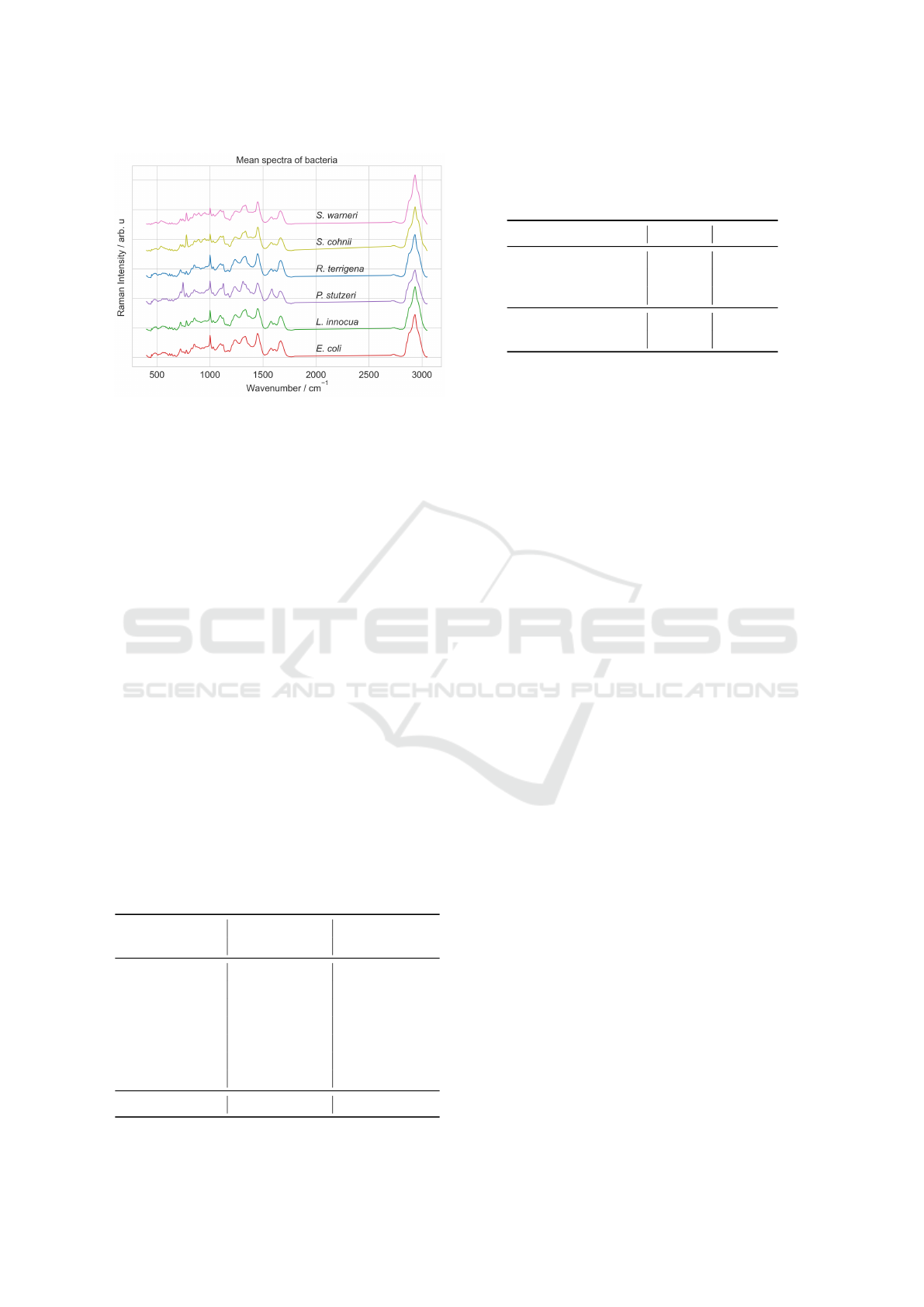
Figure 3: Mean spectra of bacteria dataset.

preprocessed spectra with 584 wavenumbers, Figure

3 shows the mean spectra for each class.

The preprocessing consists of cosmic spikes re-

moval, wavenumber calibration, spectra aligned be-

tween 240–3190 cm–1, and baseline correction. All

species were cultivated in nine independent biologi-

cal replicates (batches). Accordingly, we evaluated

by cross-validation, where the test set is composed of

two batches, and the remaining (7 batches) are used

for training (70%) and validation (30%).

We compare two CNN models trained from

scratch, a traditional 1D CNN and a transformer base

model (TrCNN) (Vaswani et al., 2017). The CNN

comprises a feature extraction part (convolutional lay-

ers) and the classiﬁcation part (dense layers). The Tr-

CNN comprises multi-head attention layers for fea-

ture extraction and dense layers for classiﬁcation.

Table 1 presents both models’ mean sensitivity ob-

tained for cross-validation on a total of 36 models.

The CNN model has a mean sensitivity of 83.05%

with a standard deviation of 4.08%, while the mean

sensitivity of the TrCNN was 82.06% with a standard

deviation of 5.34%.

Table 1: Sensitivities of all classes for the ﬁrst fold in Per-

cent (%). Cross-validation mean sensitivity for the CNN

and Transformer (TrCNN) model.

CNN TrCNN

Class Test Train Test Train

E. coli 68.87 100 51.53 92.0

L. innocua 97.57 100 96.60 90.0

P. stutzeri 88.00 100 80.00 100.0

R. terrigena 57.84 100 88.23 94.12

S. cohnii 93.93 100 84.84 98.11

S. warneri 89.10 100 89.60 97.10

AVG Sens 82.55 100 81.80 95.22

CV-Mean Sens 83.05± 4.08 82.06±5.34

Table 2: Mean absolute error (MAE) of the logits expresses

the difference between a target model and the Volterra ap-

proximation on the bacteria spectra dataset. The number of

parameters for the target models and Volterra network.

Model CNN TrCNN

MAE Train 0.5040 0.2174

MAE Validation 1.3211 0.4119

MAE Test 1.2521 0.3874

Model parameters 19.5M 104.4K

Volterra parameters 175.2K 175.2K

Table 1 also reports the average and the sensitivity

of all classes for the ﬁrst fold. The average sensitiv-

ity of batch 0 is close to the mean cross-validation

sensitivity, indicating that it is a successfully trained

model. The traditional 1D CNN performs slightly

better. Nevertheless, note that the number of CNN

parameters used is signiﬁcantly higher (19.5 M) than

the TrCNN model parameters (104.4 K), as shown in

table 2.

4.1.1 1D Volterra Approximation

We evaluate the models trained on the ﬁrst fold using

our Volterra method. Although the models have dif-

ferent architectures and parameters, we used the same

architecture in our Volterra network to approximate

both models. A better approximation can be found

by parameter selection. The tanh activation function

at the last Volterra layer transforms the output values

from −1 to 1. These values are combined linearly us-

ing a dense layer to approximate the logit values of

the original models. This linear combination can be

visualized as a relevance map or saliency map.

Table 2 exhibits the approximation error, which is

the difference between the target model output and the

Volterra approximation. As expected, the errors of the

transformer model (Tr-CNN) are much lower. This

model has fewer parameters and has a slightly lower

performance than the CNN model, with 104.4K pa-

rameters, while the CNN has 19.5M parameters. The

two Volterra models are identical. The approximation

error can be reduced by increasing the number of pa-

rameters, layers, or training strategies.

Figure 4 shows examples of two saliency maps for

the CNN model generated using our Volterra approx-

imation and a Taylor-based (Montavon et al., 2017)

method. Each saliency map is divided into two sec-

tions. The top part corresponds to the classiﬁer pre-

diction, and the bottom corresponds to the ground

truth class.

The spectra in Figure 4a correspond to the E. coli

class, but is wrongly classiﬁed as R. terrigena. Cor-

rectly classiﬁed spectra have equal saliency maps, as

ICPRAM 2023 - 12th International Conference on Pattern Recognition Applications and Methods

600

a. Wrongly classiﬁed spectra.

b. Correctly classiﬁed spectra.

Figure 4: Saliency Map for the CNN model generated using

the Volterra approximation (top) and a Taylor-based (Mon-

tavon et al., 2017) method (bottom). Each saliency map

is divided into two sections. The top part corresponds to

the classiﬁer prediction, and the bottom corresponds to the

ground truth class.

shown in Figure 4b. For the predicted class, the areas

with dark red are the areas that inﬂuence the most,

while the areas in yellow are less important for the

classiﬁcation. Simultaneously, for the correct class,

the bands that inﬂuence the most are magenta, and

the bands that inﬂuence the least are cyan.

The Volterra approximation error is an indicator of

the saliency map quality. A small error indicates that

the input is close to the expected spectra for that class.

The information provided for saliency maps is difﬁ-

cult to read, especially for the Taylor method, which

displays excessive noise. We can see that the result

does not focus on the areas as our method does.

We consider that a better manner to examine

this output is to focus only on the k most relevant

wavenumbers. Figure 5 shows the top 15 spectra

(wavenumbers) for the CNN model obtained using

our Volterra method (top) and the Taylor method (bot-

tom). Figure 5a shows an example of a misclassiﬁed

spectrum. The spectra in Figure 5b were correctly

classiﬁed, and the difference between the target model

output and the Volterra approximation is 0.07, which

corresponds to 2.25%.

Figure 6 shows histograms constructed using the

training data, which accumulate the k most important

wavenumbers for two classes (E. coli and L. innocua).

a. Wrongly classiﬁed spectra.

b. Correctly classiﬁed spectra.

Figure 5: K most relevant wavenumber postions (variables)

for the CNN model obtained using our Volterra method

(top) and the Taylor method (bottom). Each saliency map

is divided into two sections. The top part corresponds to

the classiﬁer prediction, and the bottom corresponds to the

ground truth class.

The red areas indicate the most frequently used bands

by the classiﬁer according to the Volterra and Taylor-

based methods.

Figure 6: Histograms accumulate the kth most important

wavenumbers for the CNN model. (a) Volterra approxima-

tion, (b) Taylor-based method. The red areas indicate the

most frequently used bands by the CNN model.

Agnostic eXplainable Artiﬁcial Intelligence (XAI) Method Based on Volterra Series

601

The bands shown by the Volterra model are more

concentrated, while the bands used by the Taylor

method are highly distributed. Taylor-based models

should theoretically select a root point value; by ap-

proximating this value, the results are only guaran-

teed stable for some cases. Some recent variations

of the Taylor method, such as layer-wise backpropa-

gation, employ rules to select a reference point and

to omit negative gradients or enhance positive ones.

However, there needs to be a deﬁned way to establish

whether the generated map is reliable. On the other

hand, in this work, we use the Volterra approximation

to state directly the cases in which our model deviates

too much from the original model, so the result should

not be considered.

4.2 2D Images

We assess our 2D Volterra model on two datasets,

CIFAR-10 (Krizhevsky et al., 2009), and a public

histology dataset (Kather et al., 2016). Hundreds of

methods are used for image classiﬁcation. In this pa-

per, we select two models, a popular transfer learning

strategy and a transformer-based network in the top

5 state-of-the-art. Both models can be improved by

changing the architecture, increasing the number of

layers, by parameters such as the learning rate sched-

ule, optimizer, weight decay, or data augmentation.

However, our interest is not to train the best network,

but to evaluate previously trained networks.

Transfer learning. This CNN network performs

transfer learning based on one of the most com-

mon pre-trained networks, the ResNet50, available in

Keras, where the weights are pre-trained in Imagenet.

All layers are retained except the ﬁnal classiﬁcation

layers, replaced by two dense layers with non-linear

activation ReLU and the last layer with Softmax acti-

vation.

Transformer-based network. We implemented Tr-

CNN, a version of the Vision Transformer (ViT)

model proposed by (Dosovitskiy et al., 2020) for

image classiﬁcation. TrCNN uses the self-attentive

Transformer architecture, which requires images to be

transformed into patch sequences.

4.2.1 CIFAR-10

CIFAR-10 is a benchmark dataset consisting of 60000

32 × 32 color images in 10 classes, with 6000 im-

ages per class, including airplanes, cars, birds, cats,

deer, dogs, frogs, horses, ships, and trucks. There are

50000 training images and 10000 test images. The

training dataset is divided into validation (20%) and

training (80%) splits in our experiments. The test split

contains 1000 images from each class.

Figure 7: Relevance maps and logit values for the airplane

class. (a-b) correct classiﬁcation, the error is small (rele-

vance maps can be trusted). (c) correct classiﬁcation. How-

ever, the pixels used for the estimation are incorrect. (d)

incorrect classiﬁcation, the error is large (the relevance map

cannot be trusted).

Table 3: Classiﬁcation results for CIFAR 10 dataset, mean

accuracy, top-5 accuracy. The number of parameters for the

target models and Volterra network.

Model CNN TrCNN

Mean Accuracy 82.95 64.18

Top-5 Accuracy 99.12 96.26

Model Parameters 26.1M 507.2K

Volterra Parameters 1.4M 1.4M

Table 3 shows the classiﬁcation mean accuracy

and top-5 accuracies. The accuracy for CNN (transfer

learning, Resnet-50) is lower than the typical value of

around 90%, obtained through a better learning rate

ICPRAM 2023 - 12th International Conference on Pattern Recognition Applications and Methods

602

Figure 8: Relevance maps and logit values for CNN model

and Volterra method for the CIFAR 10 dataset.

selection and a robust data augmentation strategy.

On the other hand, Alexey Dosovitskiy et al.

(Dosovitskiy et al., 2020) reported an accuracy of

99.5% achieved by pre-training the ViT model using

the JFT-300M dataset, then ﬁne-tuning it on CIFAR

10, in our case, we trained the network from scratch,

obtaining only accuracy of 64.18% and top 5 accura-

cies of 96.26% as shown in Table 3.

Table 4 summarizes the logit errors.

Table 4: Mean absolute error of the logits on CIFAR 10

dataset, which expresses the difference between the models

and the Volterra approximation.

Model Train Validation Test

CNN 0.5040 1.3211 1.2521

TrCNN 0.2174 0.4119 0.3874

Figure 9: Relevance maps and logit values for the CNN

model and Volterra method for the class dog.

We employ the mean absolute error to measure the

difference between the models and the Volterra ap-

proximation logits, which have a dynamic range.

The CNN error is greater than the error for the Tr-

CNN, because it is more complex, with 26.1M param-

eters, while TrCNN has just 500K, and our Volterra

network uses only 1.4M.

Figure 7 shows relevance maps obtained using our

Volterra method for images of the airplane class. The

logit for the CNN, TrCNN, and the Volterra approxi-

mation method. The larger the logit value for the orig-

inal model, the more it indicates that the class is an

airplane. The prediction of the original model for Fig-

ure 7a and Figure 7b are correct. We can observe that

the pixels that belong to the planes are shown with

more intensity. Consequently, the model is paying at-

tention to the right place. Additionally, the Volterra

approximation error is small. Therefore, the relevance

map can be trusted. The classiﬁcation of Figure 7c is

correct. However, the relevance map shows that the

classiﬁcation is based on the shape of the black pixels

at the edge of the image, which are artifacts and possi-

bly correspond to the window from which the picture

was taken. The original model’s prediction in Figure

7d is incorrect. The logit corresponding to the class

airplane is negative, and the model classiﬁed it as a

Agnostic eXplainable Artiﬁcial Intelligence (XAI) Method Based on Volterra Series

603

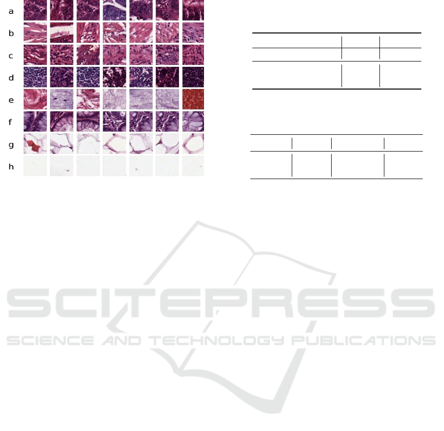
Figure 10: Images of every tissue class from the stained

colorectal cancer histology dataset (Kather et al., 2016). (a)

tumour epithelium, (b) simple stroma, (c) complex stroma,

(d) immune cell conglomerates, (e) debris and mucus, (f)

mucosal glands, (g) adipose tissue, and (h) background.

ship. In this case, the highlighted pixels belong to the

background (sky and mountains). Fortunately, we can

use this large Volterra approximation error to indicate

that this relevance map should not be trusted.

Figure 8 shows additional relevance maps for cor-

rect predictions of images for the classes bird and

horse. Figure 8c and Figure 8d show that humans are

the most relevant pixels to classify these images as

horses. However, humans are not present in CIFAR-

10 as a class, but there are several images where they

ride horses, showing a clear example of bias.

Figure 9 shows tested images not from the dataset,

with humans and dogs. Dogs are correctly classiﬁed

if humans are next to them, as shown in Figure 9a.

However, when the humans are on top, the classiﬁer

gets confused, and some are classiﬁed as horses. Fig-

ure 9b is correctly classiﬁed. However, the model is

almost equally conﬁdent that the image is a dog or a

horse with logit values equal to 4.08 and 3.10. Fig-

ure 9c is classiﬁed as a horse, which shows that the

relevance maps in Figure 9 classify were correct.

4.2.2 Colorectal Dataset

The H&E stained colorectal cancer histology dataset

(Kather et al., 2016) has eight different classes: tumor

epithelium, simple stroma, complex stroma (stroma

containing single tumor cells and/or single immune

cells), immune cell conglomerates, debris and mucus,

mucosal glands, adipose tissue, and background. The

images are tissue tiles at different scales ranging from

individual cells, with an approximate size of 10 µm,

e.g., Figure 10 (d) to larger structures such as mu-

Table 5: Accuracy on stained histology dataset (in Percent),

number of parameters for the target models and Volterra

network.

Model CNN TrCNN

Accuracy 92.4 79.20

Model Parameters 26.2M 703.6K

Volterra Parameters 6.4M 6.4M

Table 6: Mean absolute error (MAE) of the logits expresses

the difference between a target model and the Volterra ap-

proximation on the stained histology dataset.

Model Train Validation Test

CNN 0.0108 0.0636 0.0617

TrCNN 0.0114 0.1013 0.0992

cosal glands ≥ 50 µm, e.g., Figure 10 (f). The dataset

has 5000 images, 3200 were used for training, 800 for

validation, and 1000 for testing. The size of the RGB

images is 224 × 224. The models were trained from

scratch without data augmentation during 200 epochs.

Table 5 shows the mean accuracy and the number

of parameters for the CNN, TrCNN, and Volterra net-

work. The CNN accuracy is signiﬁcantly higher than

the TrCNN model. Although TrCNN is a newer and

state-of-the-art model, this network is trained from

scratch and has no pre-training. The results for both

models can be improved using different strategies.

However, our interest is to analyze trained models.

Table 6 presents the approximation mean abso-

lute error, which measures the difference between the

models and their Volterra approximation. The errors

are low, and the validation and testing errors are in the

same range and not too far from the training error. We

use identical Volterra models even though the models

are different. The Volterra model can be more or less

complex if a more precise approximation is required.

However, the approximation found is satisfactory.

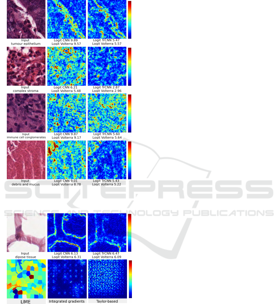
Figure 11 displays relevance maps obtained by

our method on the CNN and TrCNN. In most cases,

Volterra’s logit is remarkably close to the target

model. In the relevance maps, dark blue indicates

that the pixels are less inﬂuential, and red indicates

greater relevance. Background class, and some tis-

sues such as debris and mucus (see Figure 11d), con-

tain homogeneous texture, so the relevance is dis-

tributed throughout the image, except for some areas

in red that break homogeneity. Figure 11b and Fig-

ure 11c are opposite, while Figure 11b should high-

light only the stroma (note that the relevance map in-

dicates in blue that cells are being ignored). Figure

11c should omit the stroma and look at the immune

cell conglomerates.

ICPRAM 2023 - 12th International Conference on Pattern Recognition Applications and Methods

604

Figure 11: Histology dataset, relevance maps and logits (a)

tumour epithelium, (b) complex stroma, (c) immune cell

conglomerates, and (d) debris and mucus.

Figure 12: Histology dataset, explanations for adipose tis-

sue. (a) Input and Volterra relevance maps, (b) Comparison

with existing approaches.

Figure 12 compares the relevance map obtained

for our Volterra XAI method and other existing ap-

proaches for adipose tissue. Texture and color are

not relevant to our method for the lipid class (see Fig-

ure 12a). The edges of the lipids that form structures

and lines allow this class to be classiﬁed. In contrast,

LIME (Mishra et al., 2017) exhibits an output with

few details because it is based on the search for rele-

vant regions. The results obtained by integrated gra-

dients (Sundararajan et al., 2017) and Taylor-based

(Montavon et al., 2017) method are hardly inter-

pretable. Gradient methods describe pixel changes in

the model’s prediction and do not fully explain the

model prediction. Alternatively, Volterra relevance

maps can be used directly by more experienced users

(physicians) who can check the models for biases.

5 CONCLUSIONS

We propose an agnostic explainable artiﬁcial intelli-

gence method based on the Volterra series to approxi-

mate models, identify biases, and clarify model deci-

sions. The model architecture is composed of second-

order Volterra layers. To make fair comparisons from

our point of view, we used identical Volterra models

even though the target models were different. How-

ever, the Volterra model can be more or less com-

plex if a more precise approximation is required. Our

Volterra network allows us to create a simpler model

by emulating a target model. We evaluate the perfor-

mance of the emulation numerically by comparing a

target model’s prediction and the Volterra approxima-

tion. Therefore, no labels are required, and compa-

rable data can be employed even when training data

is unavailable. We generate relevance maps for Ra-

man spectra and 2D images. They explain the contri-

bution of the input elements to the prediction. The

trustworthiness of our method can be measured by

considering the error of the Volterra approximation.

We obtain low training errors for most of the models.

The validation and testing errors are in the same range

and not too far from the training error for the bacte-

ria dataset (TrCNN), histology dataset (CNN and Tr-

CNN), and CIFAR 10 (TrCNN). We present relevance

maps indicating higher and lower contributions to the

approximation prediction (logit) for commonly used

models. We identify biases in the models trained on

the CIFAR 10 dataset, which allows us to eliminate

them. Despite this does not seem transcendental for

the classiﬁcation of simple classes, bias identiﬁcation

is critical in the medial area.

ACKNOWLEDGEMENTS

This work is supported by the Ministry for Eco-

nomics, Sciences and Digital Society of Thuringia

(TMWWDG), under the framework of the Lan-

desprogramm ProDigital (DigLeben-5575/10-9) and

the Federal Ministry of Education and Research

Agnostic eXplainable Artiﬁcial Intelligence (XAI) Method Based on Volterra Series

605

of Germany (BMBF), funding program Photonics

Research Germany (FKZ: 13N15466, 13N15710,

13N15708) and is integrated into the Leibniz Cen-

ter for Photonics in Infection Research (LPI). The

LPI initiated by Leibniz-IPHT, Leibniz-HKI, UKJ

and FSU Jena is part of the BMBF national roadmap

for research infrastructures.

REFERENCES

Ali, N., Girnus, S., R

osch, P., Popp, J., and Bocklitz, T.

(2018). Sample-size planning for multivariate data: a

raman-spectroscopy-based example. Analytical chem-

istry, 90(21):12485–12492.

Azpicueta-Ruiz, L. A., Zeller, M., Figueiras-Vidal, A. R.,

Arenas-Garcia, J., and Kellermann, W. (2010). Adap-

tive combination of volterra kernels and its application

to nonlinear acoustic echo cancellation. IEEE Trans-

actions on Audio, Speech, and Language Processing,

19(1):97–110.

Bach, S., Binder, A., Montavon, G., Klauschen, F., M

uller,

K.-R., and Samek, W. (2015). On pixel-wise explana-

tions for non-linear classiﬁer decisions by layer-wise

relevance propagation. PloS one, 10(7):e0130140.

Bocklitz, T. (2019). Understanding of non-linear parametric

regression and classiﬁcation models: A taylor series

based approach. In ICPRAM, pages 874–880.

Dosovitskiy, A., Beyer, L., Kolesnikov, A., Weissenborn,

D., Zhai, X., Unterthiner, T., Dehghani, M., Minderer,

M., Heigold, G., Gelly, S., et al. (2020). An image is

worth 16x16 words: Transformers for image recogni-

tion at scale. arXiv preprint arXiv:2010.11929.

Franz, M. O. and Sch

olkopf, B. (2006). A unifying view

of wiener and volterra theory and polynomial kernel

regression. Neural computation, 18(12):3097–3118.

Halicek, M., Dormer, J. D., Little, J. V., Chen, A. Y., and

Fei, B. (2020). Tumor detection of the thyroid and

salivary glands using hyperspectral imaging and deep

learning. Biomedical Optics Express, 11(3):1383–

1400.

Kather, J. N., Weis, C.-A., Bianconi, F., Melchers, S. M.,

Schad, L. R., Gaiser, T., Marx, A., and Z

ollner, F. G.

(2016). Multi-class texture analysis in colorectal can-

cer histology. Scientiﬁc reports, 6(1):1–11.

Khatri, C. and Rao, C. R. (1968). Solutions to some func-

tional equations and their applications to characteriza-

tion of probability distributions. Sankhy

a: The Indian

Journal of Statistics, Series A, pages 167–180.

Korenberg, M. J. and Hunter, I. W. (1996). The identiﬁ-

cation of nonlinear biological systems: Volterra ker-

nel approaches. Annals of biomedical engineering,

24(2):250–268.

Krizhevsky, A., Hinton, G., et al. (2009). Learning multiple

layers of features from tiny images.

Lin, H., Deng, F., Zhang, C., Zong, C., and Cheng, J.-X.

(2019). Deep learning spectroscopic stimulated raman

scattering microscopy. In Multiphoton Microscopy in

the Biomedical Sciences XIX, volume 10882, pages

207–214. SPIE.

Lundberg, S. M. and Lee, S.-I. (2017). A uniﬁed approach

to interpreting model predictions. Advances in neural

information processing systems, 30.

Mishra, S., Sturm, B. L., and Dixon, S. (2017). Local inter-

pretable model-agnostic explanations for music con-

tent analysis. In ISMIR, volume 53, pages 537–543.

Montavon, G., Lapuschkin, S., Binder, A., Samek, W., and

uller, K.-R. (2017). Explaining nonlinear classiﬁca-

tion decisions with deep taylor decomposition. Pat-

tern recognition, 65:211–222.

Niioka, H., Asatani, S., Yoshimura, A., Ohigashi, H.,

Tagawa, S., and Miyake, J. (2018). Classiﬁcation of

c2c12 cells at differentiation by convolutional neural

network of deep learning using phase contrast images.

Human cell, 31(1):87–93.

Orcioni, S. (2014). Improving the approximation ability

of volterra series identiﬁed with a cross-correlation

method. Nonlinear Dynamics, 78(4):2861–2869.

Orcioni, S., Terenzi, A., Cecchi, S., Piazza, F., and Carini,

A. (2018). Identiﬁcation of volterra models of tube au-

dio devices using multiple-variance method. Journal

of the Audio Engineering Society, 66(10):823–838.

Rodner, E., Bocklitz, T., von Eggeling, F., Ernst, G., Cher-

navskaia, O., Popp, J., Denzler, J., and Guntinas-

Lichius, O. (2019). Fully convolutional networks in

multimodal nonlinear microscopy images for auto-

mated detection of head and neck carcinoma: Pilot

study. Head & neck, 41(1):116–121.

Seber, G. A. (2008). A matrix handbook for statisticians.

John Wiley & Sons.

Simonyan, K., Vedaldi, A., and Zisserman, A. (2013).

Deep inside convolutional networks: Visualising im-

age classiﬁcation models and saliency maps. arXiv

preprint arXiv:1312.6034.

Stegmayer, G. (2004). Volterra series and neural networks

to model an electronic device nonlinear behavior. In

2004 IEEE International Joint Conference on Neu-

ral Networks (IEEE Cat. No. 04CH37541), volume 4,

pages 2907–2910. IEEE.

Stegmayer, G., Pirola, M., Orengo, G., and Chiotti, O.

(2004). Towards a volterra series representation from

a neural network model. WSEAS Transactions on Sys-

tems, 3(2):432–437.

Sundararajan, M., Taly, A., and Yan, Q. (2017). Axiomatic

attribution for deep networks. In International confer-

ence on machine learning, pages 3319–3328. PMLR.

Vaswani, A., Shazeer, N., Parmar, N., Uszkoreit, J., Jones,

L., Gomez, A. N., Kaiser, Ł., and Polosukhin, I.

(2017). Attention is all you need. Advances in neural

information processing systems, 30.

ICPRAM 2023 - 12th International Conference on Pattern Recognition Applications and Methods

606