Sampling-Distribution-Based Evaluation for Monte Carlo Rendering

Christian Freude

, Hiroyuki Sakai

, K

aroly Zsolnai-Feh

and Michael Wimmer

Institute of Visual Computing and Human-Centered Technology, TU Wien, Favoritenstr. 9-11 / E193-02, Vienna, Austria

Keywords:

Computer Graphics, Rendering, Ray Tracing, Evaluation, Validation.

Abstract:

In this paper, we investigate the application of per-pixel difference metrics for evaluating Monte Carlo (MC)

rendering techniques. In particular, we propose to take the sampling distribution of the mean (SDM) into

account for this purpose. We establish the theoretical background and analyze other per-pixel difference

metrics, such as the absolute deviation (AD) and the mean squared error (MSE) in relation to the SDM.

Based on insights from this analysis, we propose a new, alternative, and particularly easy-to-use approach,

which builds on the SDM and facilitates meaningful comparisons of MC rendering techniques on a per-pixel

basis. In order to demonstrate the usefulness of our approach, we compare it to commonly used metrics based

on a variety of images computed with different rendering techniques. Our evaluation reveals limitations of

commonly used metrics, in particular regarding the detection of differences between renderings that might be

difﬁcult to detect otherwise—this circumstance is particularly apparent in comparison to the MSE calculated

for each pixel. Our results indicate the potential of SDM-based approaches to reveal differences between

MC renderers that might be caused by conceptual or implementation-related issues. Thus, we understand our

approach as a way to facilitate the development and evaluation of rendering techniques.

1 INTRODUCTION

Simulating light transport for the synthesis of pho-

torealistic images is of great importance for ﬁlm

production, architectural visualization, product de-

sign, and many other applications. Predominant ap-

proaches to solve this problem are based on a model

described by the rendering equation (Kajiya, 1986)

and evaluate its numerous integrals using Monte

Carlo (MC) integration.

This type of integration approximates the integral

of a function through exhaustive random sampling.

Due to the stochastic nature of this approach, the ap-

proximations generally suffer from variance, which

manifests itself as noise in the rendered images. As

the number of samples increases, the variance eventu-

ally vanishes and the integral converges to the correct

solution.

A signiﬁcant amount of research has been dedi-

cated to reduce variance and speed up convergence

by using more advanced sampling strategies. How-

ever, the variance inherent to all MC-based render-

ing techniques impedes their comparison, as images

https://orcid.org/0000-0002-4224-4105

https://orcid.org/0000-0003-0388-8458

https://orcid.org/0000-0003-3707-6319

https://orcid.org/0000-0002-9370-2663

are only completely noise-free in the theoretical limit,

which generally cannot be attained in practice. More-

over, commonly used difference metrics do not take

this variance fully into account.

In this paper, we investigate the potential of sam-

pling distribution-based approaches for the compari-

son and evaluation of MC renderings and techniques

on a per-pixel basis. The key insight is that conven-

tional metrics, such as the absolute deviation (AD) or

mean squared error (MSE), only incorporate limited

information about the distributions of per-pixel radi-

ance estimates. We see great potential in incorporat-

ing additional information, in particular information

about the sampling distribution of the mean (SDM),

to develop improved measures that can reveal differ-

ences more clearly than other approaches. The under-

lying intuition is that the SDM includes information

about the variability of per-pixel radiance estimates at

a particular stage of convergence, i.e., for a particular

number of samples per pixel (SPP). Therefore, the ac-

curacy of the renderings can be incorporated into the

measure and leveraged for comparison.

We propose a novel, alternative approach that

builds on the estimation of the SDM. It essentially

estimates the probability that one integrator produces

similar radiance estimates as another. Our approach

can be used for effectively comparing and evaluating

Freude, C., Sakai, H., Zsolnai-Fehér, K. and Wimmer, M.

Sampling-Distribution-Based Evaluation for Monte Carlo Rendering.

DOI: 10.5220/0011886300003417

In Proceedings of the 18th International Joint Conference on Computer Vision, Imaging and Computer Graphics Theory and Applications (VISIGRAPP 2023) - Volume 1: GRAPP, pages

119-130

ISBN: 978-989-758-634-7; ISSN: 2184-4321

 2023 by SCITEPRESS – Science and Technology Publications, Lda. Under CC license (CC BY-NC-ND 4.0)

119

(a) Unbiased Reference (b) Biased Rendering (c) Per-Pixel Root Mean

Squared Error

(d) Our Approach for

Evaluation

Figure 1: Here, we illustrate the potential of our proposed approach for the evaluation of Monte Carlo (MC) rendering

techniques. It is based on the sampling distribution of the mean (SDM). Image (a) shows a reference rendering and (b) an

artiﬁcially biased rendering for which the reﬂectance of the couch on the right-hand side was reduced. Our approach (d) can

reveal differences between both renderings that are difﬁcult to identify through visual comparison or other metrics, e.g., the

(normalized) root mean squared error (RMSE) calculated for each pixel (c). This circumstance suggests the viability of using

SDM-based approaches for the per-pixel comparison of MC renderings.

MC renderings and techniques (see Figure 1).

The closely related work by Jung et al. (Jung

et al., 2020) already demonstrated how statistical ap-

proaches can be used effectively to reveal bias in ren-

dered images. They show that a non-uniform distri-

bution of p-values (based on the Welch’s test statistic)

is an indicator for bias. In contrast, we compute the

probability that one renderer computes similar radi-

ance values as another and moreover facilitate mean-

ingful comparisons between unbiased integrators. We

see our approach as an alternative to the work by Jung

et al.

The remainder of our paper is structured as fol-

lows: In Section 2, we provide an overview over re-

lated work. To motivate the incorporation of addi-

tional statistical information, such as the SDM, we

discuss the statistical background and provide a theo-

retical comparison of different measures in Section 3.

In Section 4, we present our approach. Furthermore,

in Section 5, we evaluate the measures based on ren-

derings of several scenes computed by different inte-

grators. Our examples illustrate how well the mea-

sures are able to reveal differences between render-

ings. We show that sampling-distribution-based mea-

sures are consistently able to reveal subtle differences.

Moreover, we point out shortcomings of per-pixel

mean squared error (ppMSE) in particular.

2 RELATED WORK

In previous work, researchers proposed various meth-

ods for the comparison and evaluation of Monte Carlo

(MC) renderings. In the following, we provide an

overview over those methods.

Perceptual Metrics. Many researchers employed a

perceptual model that can be used to approximate per-

ceived differences, which in turn can be exploited for

rendering. For instance, the visible differences pre-

dictor (Daly, 1993) has been employed to approx-

imate perceived rendering quality in order to use

it for a stopping condition (Myszkowski, 1998) or

to alternate between complementary rendering tech-

niques (Volevich et al., 2000). Ramasubramanian et

al. (Ramasubramanian et al., 1999) developed a per-

ceptual error metric for image-space adaptive sam-

pling. Farrugia and P

eroche (Farrugia and P

eroche,

2004) used an existing vision model (Pattanaik et al.,

1998) in order to achieve the same goal. Andersson

et al. (Andersson et al., 2020) presented an approach

that can estimate the perceived difference while al-

ternating between two images. In contrast, we focus

on the direct comparison of radiance estimates, as we

strive for objective and quantitative assessments for

MC rendering.

General Image Quality Metrics. Most researchers

leveraged general image quality metrics, which are

popular in the image-processing community, to com-

pare MC renderings. Prominent examples are the

mean squared error (MSE), the root mean squared er-

ror (RMSE), peak signal-to-noise ratio (PSNR), the

structural similarity (SSIM) index (Wang et al., 2004),

and variants of the high-dynamic-range visual differ-

ence predictor (HDR-VDP) (Mantiuk et al., 2005;

Mantiuk et al., 2011; Narwaria et al., 2015). For

instance, Meneghel and Netto (Meneghel and Netto,

2015) employed SSIM and HDR-VDP2 for the com-

parison of six different rendering techniques.

GRAPP 2023 - 18th International Conference on Computer Graphics Theory and Applications

120

Whittle et al. (Whittle et al., 2017) provided a

comprehensive overview and analysis of a multitude

of general image quality metrics. The problem with

such general metrics is that they are agnostic to the

sample distributions in MC rendering, which can po-

tentially provide a breadth of additional information.

By incorporating information about distributions, we

strive to provide a better alternative to those metrics.

Rendering Veriﬁcation. Several works (Goral

et al., 1984; McNamara et al., 2000; Schregle and

Wienold, 2004; Meseth et al., 2006; McNamara,

2006; B

arz et al., 2010; Jones and Reinhart, 2017;

Clausen et al., 2018) compare renderings to real-

world measurements in order to assess rendering

quality. Ulbricht et al. (Ulbricht et al., 2006) inves-

tigated the state of the art for the veriﬁcation of ren-

derings and pointed out that all approaches have their

weaknesses and that the development of robust and

practical solutions is still an open task. Nevertheless,

the veriﬁcation of rendering techniques using real-

world measurements is orthogonal to our goal of com-

paring different rendering techniques.

Statistical Approaches. Compared to the methods

discussed so far, statistical approaches are most rel-

evant to ours. Celarek et al. (Celarek et al., 2019)

proposed an approach to estimate MSE expectation

and variance and to analyze the error distribution over

frequencies of MC rendering techniques. Subr and

Arvo (Subr and Arvo, 2007) employed statistical tests

to compare rendering techniques. However, they used

test hypotheses that are not suited to test for equality

but can only show signiﬁcant differences. The method

by Jung et al. (Jung et al., 2020) also builds on clas-

sical hypothesis testing—speciﬁcally, Welch’s test—

by considering non-uniform distributions of p-values

as indicators for bias. Welch’s test also incorporates

more information about sampling distributions, which

makes it comparable to our proposed approach. How-

ever, our approach is not based on p-values but com-

putes probabilities that one renderer produces radi-

ance estimates similar as another. Furthermore, it

can also be used to compare unbiased renderers. In

Section 5, we discuss the differences between the ap-

proach by Jung et al. and ours in more detail.

In general, there has been a surprisingly low

amount of research on statistical approaches to com-

pare MC renderings and rendering techniques. Thus,

with our approach, we aim not only to provide a

novel, useful alternative to existing approaches but

also to inspire further research in this direction.

3 BACKGROUND

In this section, we describe the theoretical back-

ground and analyze common difference metrics in re-

lation to the sampling distribution of the mean (SDM)

in order to motivate the use of the latter for the eval-

uation of Monte Carlo (MC) renderings. Moreover,

we discuss the closely related approach by Jung et

al. (Jung et al., 2020).

3.1 Prerequisites

A MC rendering technique generates an image by

evaluating the rendering equation for each pixel by

means of MC integration. Due to the nature of this

approach, it can only estimate the involved integrals,

which generally leads to noise in the rendered im-

age. Typically, to assess quality and performance,

a noiseless reference is computed against which the

rendered image can be compared. Such a reference

generally requires a very high sample budget to en-

sure that its error is relatively low. The difference

between the rendered image to its reference is then

quantiﬁed using metrics like absolute deviation (AD),

mean squared error (MSE), or some variant thereof,

either aggregated over the whole image or per pixel.

Aggregate vs. Per-Pixel Metrics. Usually, metrics

such as the AD or MSE are computed incorporating

all pixels to form a single scalar difference value for

an individual image with respect to a reference. This

approach is useful when images need to be compared

on the basis of a single aggregated value, but it does

not help to identify the locations where the images

are different. This can rather be achieved by using

per-pixel difference metrics.

In this work, we focus on the per-pixel compari-

son of MC renderings; thus, if not stated otherwise,

all metrics in our exposition are applied on a per-

pixel basis. One fundamental shortcoming of apply-

ing commonly used metrics per pixel is that they do

not take the accuracy or state of convergence of the

renderings into account. In the following, we illus-

trate this issue and propose a potential solution based

on the SDM, which we ﬁrst review in the next para-

graphs.

Sampling Distribution of the Mean. The samples

computed by a MC integrator for a particular pixel

can be seen as a random variable X from an arbitrary

distribution f

with an unknown population mean µ

and variance σ

. The distribution mainly depends

on the type of the integrator and the scene. During

rendering, an increasing number of samples from this

Sampling-Distribution-Based Evaluation for Monte Carlo Rendering

121

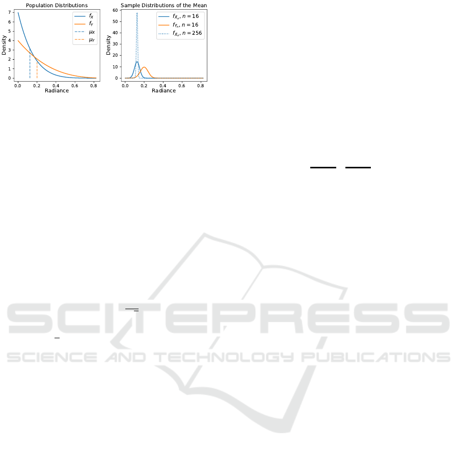
Figure 2: These plots show the relation between the popula-

tion distributions (left) and the sampling distributions of the

mean (SDMs) (right) of two random variables X (blue) and

Y (orange) representing pixel radiance samples computed

by two integrators. (For this illustration, we have used two

beta distributions for X and Y that differ slightly in mean

and variance.) According to the CLT (Equation 1), the SDM

approaches normality and decreases in standard deviation

(SD) as sample size n increases (right; dotted blue line).

distribution are averaged to estimate µ

, i.e., by com-

puting the sample mean

using n samples per pixel

(SPP).

In contrast to f

, the sampling distribution of the

mean (SDM) f

not only depends on µ

and σ

but

also on the sample size n; the central limit theorem

(CLT) states that the SDM is approximately normal-

distributed for a sufﬁciently large n:

∼ N



√



. (1)

Furthermore, the standard deviation (SD) of the SDM

= σ

√

n is known as the standard error of the

mean (SEM), which can be used to quantify the er-

ror of a MC rendering. This error is proportional to

, i.e., the SD of the integrator, and inversely pro-

portional to n. These relationships are consistent with

the fact that error can be reduced by decreasing the

SD of the integrator σ

or increasing the number of

samples n.

3.2 Issues of Commonly Used Metrics

In this section, we aim to clarify the shortcomings of

commonly used metrics such as the AD and MSE. To

this end, Figure 2 illustrates the relation between the

population distribution and the SDM. Here, random

variables X (blue) and Y (orange) represent pixel ra-

diance samples computed by two integrators. Aver-

aging transforms their population distributions (left)

into their corresponding SDMs (right). We note that

the means and therefore the bias remain unchanged.

For the same sample size n = 16, the SEMs σ

and

are proportional to the SDs of the corresponding

population distributions (both scaled by a factor of

1/4). As we increase the sample size from 16 to 256

for the sample mean

(which we hereafter consider

as the reference), the SEM σ

decreases (dotted blue

line). Therefore, the SDM inherently includes infor-

mation about the error for different states of conver-

gence.

With these considerations in mind, we now focus

on two commonly used metrics. The AD only eval-

uates |µ

−µ

|, i.e., the difference between means

(known as bias), and therefore does not include any

information about the SDM. The MSE can be written

as the sum of variance and squared bias:

MSE



θ,θ



= E





θ −θ





= E





+ E





−2θE





= E





−E





+ E





{z }





−2θE





= Var





+ E





+ θ

−2θE





= Var











−θ



= Var





+ Bias



θ,θ



(2)

where

θ is the estimator and θ is the parameter being

estimated.

Equation 2 reveals a potential shortcoming of the

MSE: one can exchange variance for bias (and vice

versa) without changing the result. Another problem

is that the MSE assumes knowledge about the pa-

rameter being estimated—in our case, the population

mean θ = µ

of the reference. In general, the pop-

ulation mean is unknown and must be estimated, but

the distribution of this estimate (the SDM) cannot be

taken into account in the MSE. Only the distribution

of the estimate

θ =

is accounted for:

MSE(

,µ

) = Var(

) + Bias(

,µ

)

. (3)

Aggregate vs. Per-Pixel MSE. We also want to

point out the key difference between applying the

MSE across all pixels of the image and applying it

per pixel. The former computes the mean squared

difference between corresponding pixels of two im-

ages and therefore tends toward zero as the difference

between those images decreases. The latter computes

the mean squared difference between random samples

and a ﬁxed reference value for each individual pixel.

Therefore, the per-pixel MSE (ppMSE) converges to

the variance plus squared bias of the used MC inte-

grator. This property makes the ppMSE less suited

for the comparison of MC renderings, as we illustrate

with the results shown in Section 5.1.

Apart from the issues mentioned so far, both AD

and MSE do not include the additional information

provided by the SDM or SEM, in particular, the ac-

curacy or state of convergence of the estimates at a

speciﬁc sample size n. This circumstance is shown

GRAPP 2023 - 18th International Conference on Computer Graphics Theory and Applications

122

Table 1: An overview of the types of information that are

considered by various difference measures (including ours).

Bias is considered by all measures. The MSE additionally

incorporates the variance of the non-reference distribution.

Our approach, as well as the one by Jung et al. (Jung et al.,

2020), moreover takes the variance of the reference distri-

bution and, more importantly, the SDMs into account.

Bias Variance Variance Sample Distr.

(non-ref.) (reference) of the Mean

AD ✔ ✘ ✘ ✘

MSE ✔ ✔ ✘ ✘

(Jung et al., 2020) ✔ ✔ ✔ ✔

SDMP (Ours) ✔ ✔ ✔ ✔

in Table 1. It includes our proposed measure, which

additionally incorporates the error of the reference,

but more importantly, is based on estimations of the

SDM to take the SEM into account. The information

that we additionally take into account can facilitate

the evaluation and comparison of different MC ren-

derings and techniques, as evidenced by the results

shown in Section 5. In addition to the metrics dis-

cussed in this section, Table 1 also includes an ap-

proach recently published by Jung et al. (Jung et al.,

2020), which we discuss in the next section.

3.3 The Approach by Jung et al.

The approach by Jung et al. (Jung et al., 2020) is

based on hypothesis testing and provides a similar

feature set as our method. It is based on Welch’s

two-sample test for the difference in means. Speciﬁ-

cally, they compute p-values for image tiles and ana-

lyze their distribution. They have shown that a non-

uniform distribution of p-values is an indicator for

bias, as under the null hypothesis (i.e., no bias), the

p-values are expected to be uniformly distributed. By

using MC samples averaged over tiles, they facilitate

the normality of the sample means, which is required

for Welch’s test.

Intuitively, a lower p-value indicates a higher

probability of the (population) means being different.

If the p-value is less than or equal to the speciﬁed

signiﬁcance level α, the difference between means is

considered signiﬁcant. But this only suggests a dif-

ference and cannot show equivalence. Nevertheless,

Jung et al. have shown that visualizing p-values per

tile can give clues about biased regions and that a uni-

form distribution of p-values indicates the absence of

bias. The similarities and differences between theirs

and our approach are discussed in Section 5, where

we also provide examples that demonstrate the advan-

tages of our approach.

4 OUR APPROACH

In the previous section, we described how the SDM

incorporates useful information about the rendering

process that is missing in classical metrics. Thus, we

propose to use the SDM for quantifying the similarity

between the radiance estimates produced by different

MC integrators. Our idea is to, for each pixel, esti-

mate the SDM and compute the probability that the

corresponding radiance estimates are similar to the

one produced by another integrator. In the following,

we derive the formulas for calculating this probability.

Probability of the Sample Mean

. We ﬁrst con-

sider a single integrator and determine the probability

that it generates sample mean values, represented by

a random variable

, in a certain range for a par-

ticular pixel. The corresponding SDM f

is deﬁned

in Equation 1. Since the probability of

taking on

any particular value in a continuous space is zero, we

can only derive probabilities for intervals (a

Given the cumulative distribution function (CDF) F

corresponding to f

, the probability that the integra-

tor produces radiance estimates in a certain interval

] can be derived as follows:

P(a

≤ b

) = P(

≤ b

) −P(

≤ a

)

= F

) −F

)

(4)

Furthermore, we consider the inverse CDF or

quantile function Q

= F

−1

, which can be used to

ﬁnd an interval that contains a certain probability

mass of the distribution. In particular, we are inter-

ested in the interval whose endpoints are equidistant

to the mean

and enclose the fraction 1 −α of all

possible values:













1 −





. (5)

This interval, which turns out to be the conﬁdence in-

terval (CI) for the sample mean, can be used to deter-

mine the probability that one integrator will produce

similar radiance estimate as another, as we describe in

the following.

Probability for Comparing Integrators. Our ap-

proach is to select one integrator (which generates

samples X) and compute the CI for its estimates

] according to Equation 5. We further de-

termine the probability that another integrator (which

generates samples Y ) produces estimates

within

this interval. Speciﬁcally, we compute how much

probability mass of the SDM of Y lies inside the CI

Sampling-Distribution-Based Evaluation for Monte Carlo Rendering

123

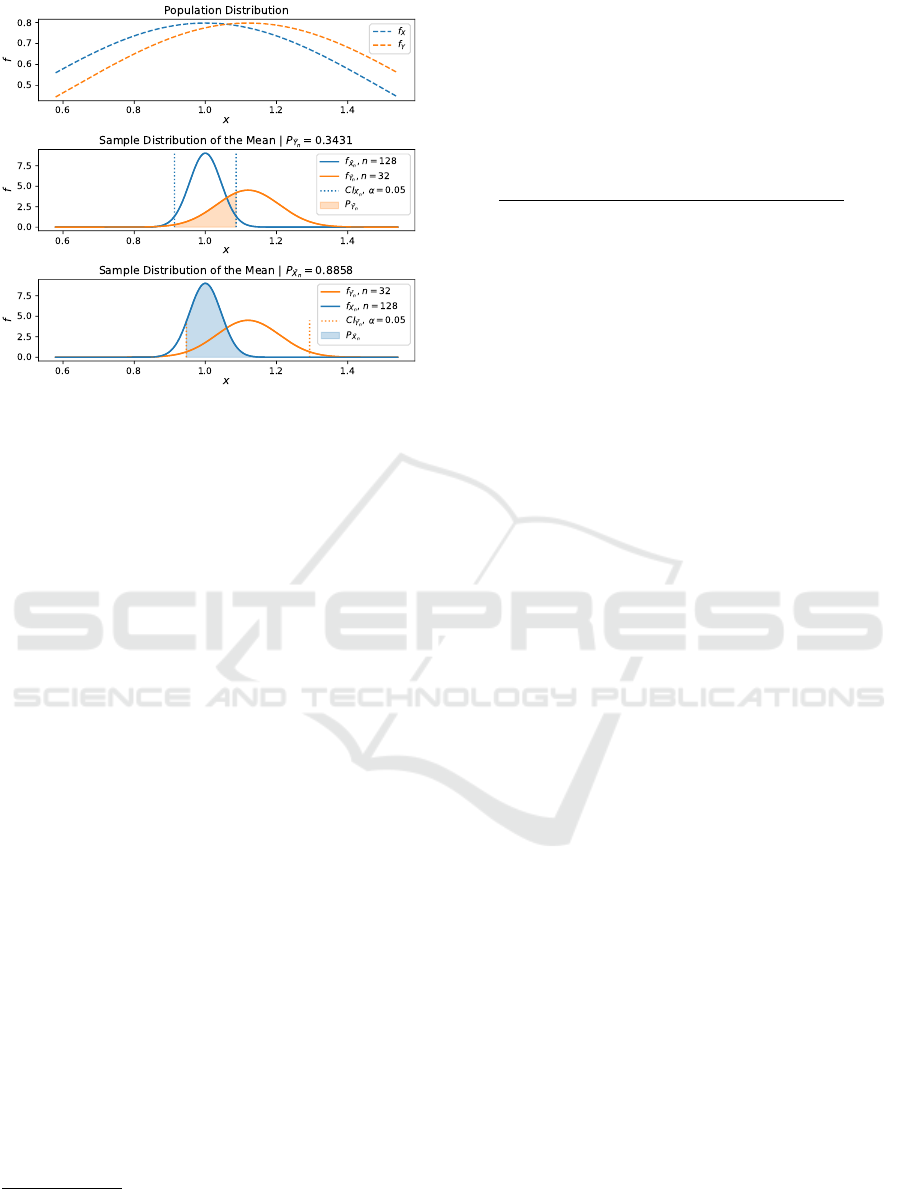
Figure 3: An illustration of the asymmetry of our approach.

At the top, population distributions for X and Y are shown,

which have equal σ but different µ. Below, corresponding

SDMs for different sample sizes for

and

are shown.

Since the SDM of X has a lower SD than that of Y , the

probabilities are not equal.

for the mean of X. This approach requires the inte-

gration of f

over the interval (a

)



≤ b



(x)dx

= F

) −F

(6)

This equation describes the probability that

takes

on values that fall into the CI for

at a conﬁdence

level 1 −α. Thus, it can be used to quantify the simi-

larity of the radiance estimates produced by two inte-

grators.

We note that this probability is not symmetric: ex-

changing

and

results in a different probability,

as illustrated in Figure 3. Intuitively, our approach

computes the overlap of one distribution with the CI

of another, which is only symmetrical if σ

= σ

We propose to choose

as the reference, for

which the error is relatively low. In this case, if

= µ

, the probability increases with the accuracy

as more of its probability mass falls into the CI

of the reference.

The corresponding probability of dissimilarity is

given by

1 −P(a

≤ b

). (7)

For our evaluation in Section 5, we have used this

dissimilarity, i.e., the probability that a test renderer

computes sample means that fall outside the CI for

Here, for brevity, we use f to denote the probability

density function (PDF) of the distribution instead of the dis-

tribution itself.

the mean of a reference renderer. We hereafter refer

to it as SDM-based probability (SDMP).

In cases where no reference is available, it may

be desirable to compare renderings on equal ground,

which would require a symmetric measure. A possi-

ble symmetric variant of our measure can be given by

the average

2 −P(a

≤ b

) −P(a

≤ b

)

. (8)

Other operations such as the minimum or maximum

of the two probabilities might also be of interest. In

this work, we focus on our asymmetric measure for

similarity and leave the investigation of symmetric

variants for future work.

Practical Considerations. In practice, since popu-

lation parameters are generally not available, our ap-

proach builds on sample estimates. Conveniently, the

required estimates can be computed online, i.e., with-

out the need to store individual samples (e.g., by us-

ing Welford’s algorithm (Welford, 1962)). For inte-

grators such as path tracing (PT), the estimates can be

directly computed from individual radiance samples

as long as the sample count is sufﬁcient to assume

normal distribution. In cases where the sample count

is insufﬁcient, we can effectively increase it by aggre-

gating over multiple pixels, as proposed by Jung et

al. (Jung et al., 2020). For more sophisticated inte-

grators such as Metropolis light transport (MLT), we

can average multiple estimates in form of short ren-

derings, as suggested by Celarek et al. (Celarek et al.,

2019).

The signiﬁcance level α can be used to control the

sensitivity of our approach, i.e., the length of the CI of

used for calculating the probability. Since the SD

of the reference renderer can be estimated in advance,

it is possible to choose the α in such a way that the CI

corresponds to a desired range of radiance values.

5 EVALUATION

In this section, we ﬁrst show how our approach com-

pares to other metrics. Afterward, we discuss the

closely related work by Jung et al. (Jung et al., 2020)

to which we also refer as JHD20 for brevity.

5.1 General Comparison

In the following, we investigate different approaches

for identifying differences in Monte Carlo (MC) ren-

derings. In particular, we compare our approach to

per-pixel absolute deviation (AD), root mean squared

GRAPP 2023 - 18th International Conference on Computer Graphics Theory and Applications

124

error (RMSE), and JHD20. (We choose RMSE in-

stead of mean squared error (MSE) since it expresses

the error in the same unit as the radiance values.)

We note that the comparisons provided in Fig-

ures 4 to 7 are structured similarly: In the ﬁrst col-

umn, we show the renderings and in the second, the

corresponding sample standard deviation (SD). The

remaining columns show images of the different ap-

proaches. The rows correspond to independently

computed renderings. The ﬁrst row corresponds to

the reference rendering (computed with a relatively

high sample count) and the others correspond to test

renderings (computed with a lower sample count).

Speciﬁcally, the second row corresponds to an unbi-

ased control rendering and the last row to an artiﬁ-

cially biased rendering, for which a scene property

has been slightly changed. For this artiﬁcial bias,

we have kept the actual integrator implementation un-

modiﬁed. Moreover, we provide the average value for

each image (shown below the label). We note that in

our ﬁgures, we show all non-radiance values as RGB

images for compact display, instead of separately dis-

playing the individual channels.

We have used 32768 SPP to compute the refer-

ence renderings and 4096 SPP in all other cases (un-

less stated otherwise). The AD and RMSE values are

bounded by [0, ∞). The p-values computed by JHD20

fall between 0 and 0.5 on average. Our approach com-

putes probabilities in the interval (0, 1). We note that

in case of JHD20, low values indicate bias, while for

the other approaches, high values indicate dissimilar-

ity. We have used the scenes provided by Bitterli (Bit-

terli, 2016).

Living Room Scene. Figure 4 shows the results for

the LIVING ROOM scene rendered using PT. For the

unbiased control rendering (second row), the AD and

the RMSE contain structures that can distract from

identifying bias. In contrast, our SDM-based proba-

bility (SDMP) and JHD20 (last two columns) show no

structure but homogeneous noise. We also illustrate

this circumstance in Figure 8, which shows that in the

frequency domain, the spectrum of both approaches

is relatively uniform compared to the AD and RMSE.

We note that since the control rendering has no

bias, the RMSE is essentially the same as the SD in

this case. This circumstance stems from the bias–

variance decomposition described in Equation 2. The

only difference is that the RMSE uses the factor 1/n

instead of 1/(n −1) for normalization.

For the biased rendering (third row), only our

SDMP and JHD20 clearly reveal the bias caused by

the sofa. In the case of the AD, the bias can be seen,

especially in comparison to the control image, but it

is accompanied by potentially distracting regions of

structured noise. For the RMSE, the biased region

cannot be visually discerned. These circumstances

demonstrate how scene features and the SD of the in-

tegrator can manifest themselves as structures in the

measures that can mask bias—a detriment that both

our SDMP and JHD20 do not suffer from.

Veach Ajar Scene. Figure 5 shows the results for

the VEACH AJAR scene rendered using BDPT. Here,

we can see, similarly to the previous LIVING ROOM

example in Figure 4, that our SDMP and JHD20

clearly reveals the bias caused by the ﬂoor, while the

AD and RMSE are less effective in this regard due to

additional potentially distracting structures.

For this scene, we also investigate the convergence

of the different approaches with increasing SPP. In

Figure 6, we can see how distracting scene structures

are visible in all AD and RMSE images. In contrast,

our SDMP and JHD20 show the bias (caused by the

ﬂoor) more clearly.

In Figure 9, plots of the corresponding average im-

age values with respect to the SPP are shown. We can

see how the average RMSE matches the correspond-

ing average SD, and that the average RMSE for the

biased rendering is (counterintuitively) lower than for

the control. This fact indicates that the RMSE is not

well-suited to identify bias. In contrast, the average

AD reveals the increase in error for the biased ren-

derings and gets more accurate with increasing sam-

ple count. JHD20 is able to show bias; however, the

average value in the control case stays constant, i.e.,

it does not show the increase in accuracy due to the

increased sample count. In contrast, our SDMP indi-

cates this increased accuracy for the control render-

ing, suggesting its use for the comparison of unbiased

renderers.

Veach Bidir Room Scene. For the last compari-

son, we have chosen the VEACH BIDIR ROOM scene,

shown in Figure 7. In this scene, the bias is caused by

a change in intensity for the spotlight that illuminates

the left-hand wall. It is imperceptible in the render-

ings as well as in the RMSE.

An interesting observation can be made by com-

paring the average values of the different measures

(below the labels). The average RMSE would (coun-

terintuitively) indicate that the biased rendering (last

row) is closer to the reference. However, the other

average values show that the unbiased rendering is

indeed more accurate than the biased one, indicating

that these measures are more suited for per-pixel com-

parison.

Sampling-Distribution-Based Evaluation for Monte Carlo Rendering

125

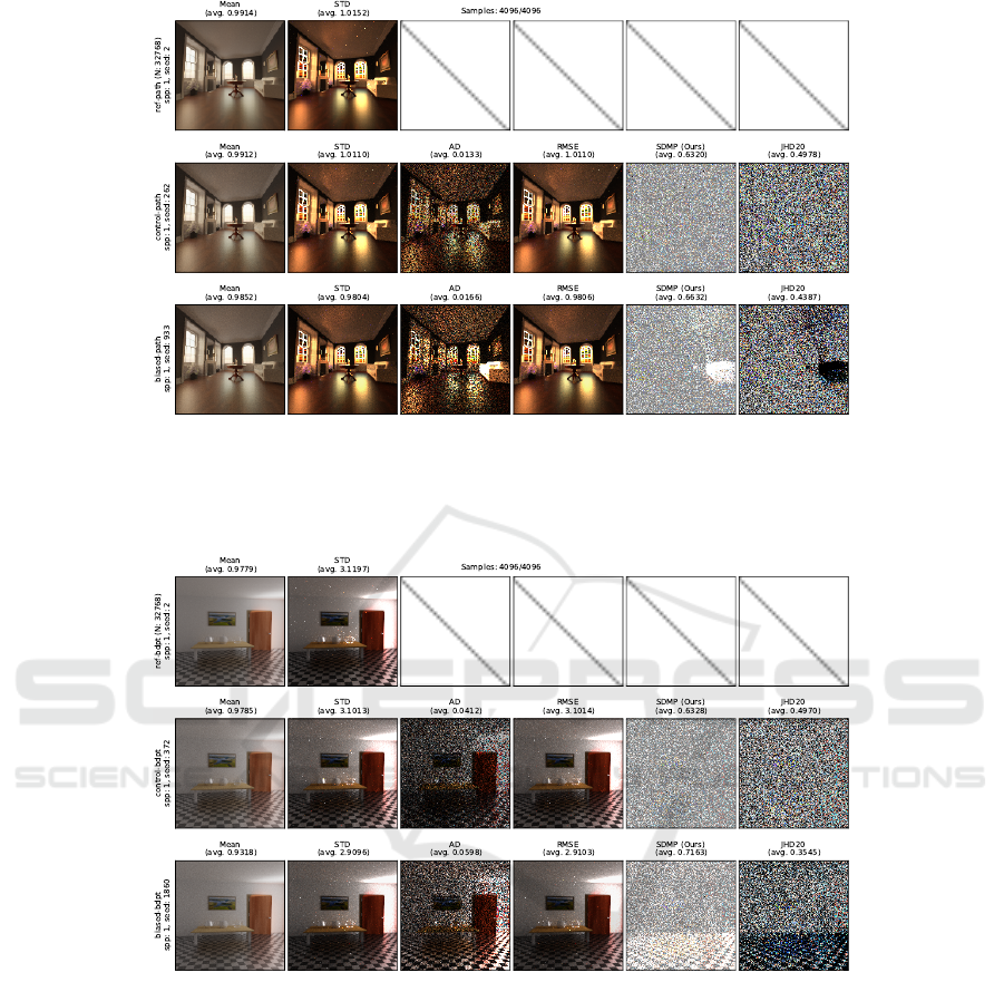
Figure 4: Renderings of the LIVING ROOM scene and the corresponding per-pixel images of different approaches for quanti-

fying the difference between renderings. All three renderings (leftmost column) were computed using path tracing (PT). The

bottom row shows an artiﬁcially biased version of the scene, for which the reﬂectance of the sofa on the right-hand side was

reduced. The structure of the scene is visible in the AD and RMSE images. Our approach and JHD20 reveal the biased image

region at the sofa (last row).

Figure 5: Renderings of the VEACH AJAR scene and the corresponding per-pixel images of different approaches for the

comparison of renderings. All three renderings (leftmost column) were computed using bidirectional path tracing (BDPT).

The third row shows an artiﬁcially biased version of the scene, for which the reﬂectance of the ﬂoor was reduced. The structure

of the scene is still visible in comparison the AD and RMSE images, while our approach and JHD20 reveal the biased image

region at the ﬂoor (last row).

Another observation is that in this scene, outliers

due to ﬁreﬂies are relatively frequent. Those addi-

tionally introduce distractions in the difference im-

ages. Moreover, they can transform the sample dis-

tributions such that the normality assumption—upon

which SDMP and JHD20 rely—is violated. We illus-

trate this issue in Figure 13 and discuss it in the next

section (5.2).

Application Scenarios. We see two main applica-

tion scenarios for our approach: The ﬁrst scenario is

the per-pixel comparison to indicate similarity or bias

in different regions of the image. The second sce-

nario is the numerical comparison based on the aver-

age SDMP, either computed across the whole image

or a region of interest.

Let us assume that we are interested in the differ-

ence between multiple renderings with respect to each

other or to a reference. The magnitude of the SDMP

image indicates the amount of difference. This differ-

ence can be visually inspected or compared numeri-

cally using values averaged over the whole or a par-

GRAPP 2023 - 18th International Conference on Computer Graphics Theory and Applications

126

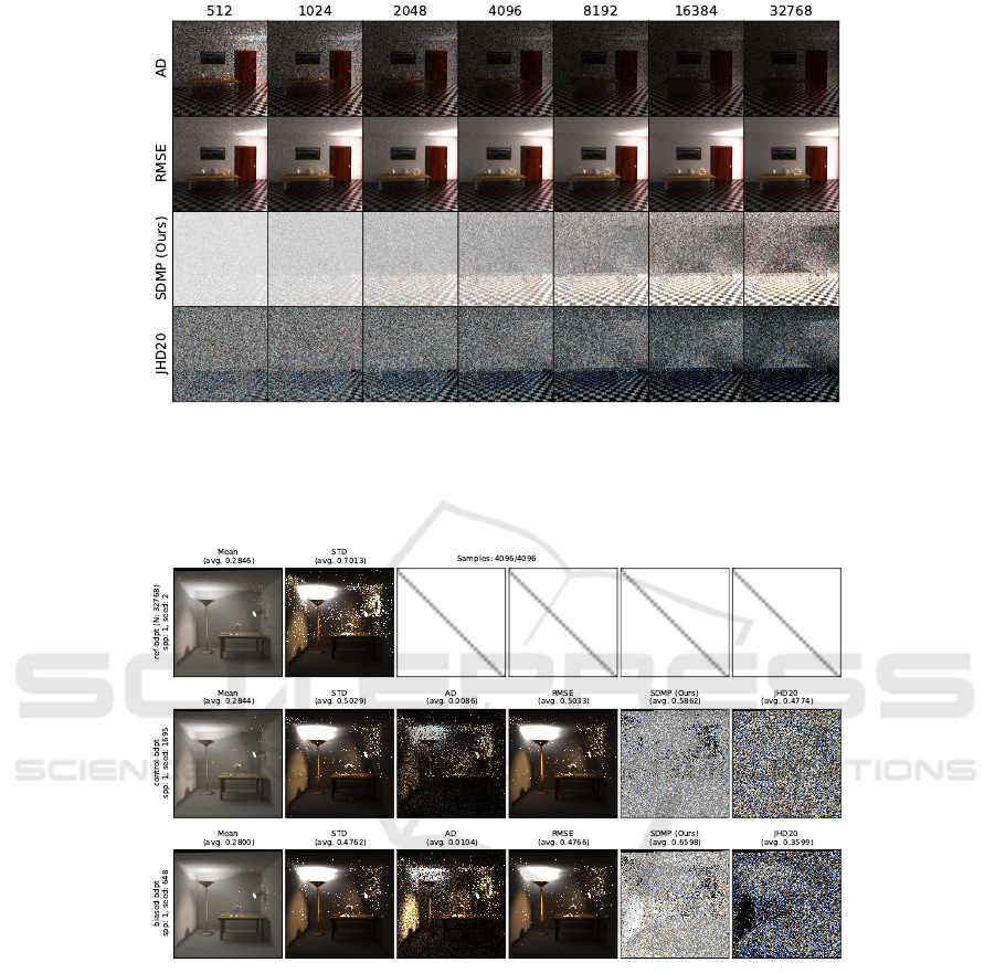
Figure 6: Images of different measures (rows) for increasing samples per pixel (SPP) (columns) for the biased variant of the

VEACH AJAR scene. Here, we can see that the AD decreases while many regions, e.g. the back wall, remain noisy. By

contrast, the noise in the RMSE images vanishes more quickly, while the images converges to the SD of the BDPT integrator.

In comparison, our approach and JHD20 reveal the bias more clearly, since other scene features are less noticeable. The

convergence of the corresponding average image values is illustrated in Figure 9.

Figure 7: Comparison of measures based on the VEACH BIDIR ROOM scene. The biased variant (bottom row) was created

by decreasing the emission of the spotlight mounted on the right-hand wall. All renderings were computed using BDPT. The

introduced bias results in an increased intensity of the illumination on the left-hand wall. Here all approaches, except RMSE,

are able to show the biased region; however, our approach and JHD20 exhibit less structure in other image regions.

ticular region of the image. We provide examples of

such visual comparisons in Figures 4 to 6 and a basic

example of numerical comparison in Figure 9.

Additional examples of numerical comparisons

are provided in Figures 10 to 11. Here, we illustrate

the properties of the SDMP in comparison to the other

measures based on the VEACH AJAR scene. We com-

pare average values of the measures with respect to

sample count. These average values are computed

across the top image region, the bottom region, and

the full image, as illustrated in Figure 12. For the un-

biased control rendering (Figure 10), AD and RMSE

exhibit different average values for each region. Our

SDMP and JHD20 exhibit the same average values

for all regions. This is due to their beneﬁcial uniform

spectrum, as shown in Figure 8.

Furthermore, it can be seen that the SDMP as-

signed a lower value (less difference) for the low-

quality reference case (dashed lines). This is be-

cause the conﬁdence interval (CI) for the low-quality

reference is much broader than the CI of the high-

quality reference and therefore includes more proba-

bility mass of the sampling distribution of the mean

(SDM) of the test rendering. This shows that our ap-

Sampling-Distribution-Based Evaluation for Monte Carlo Rendering

127

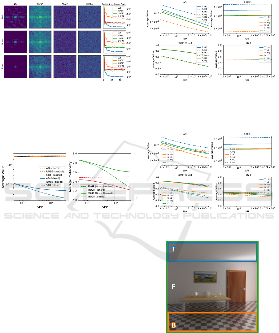
Figure 8: The fast Fourier transform (FFT) power spectra

corresponding to the control images in Figure 4. The ﬁrst

four columns (from the left) show the 2D power spectra for

each approach, while the rightmost column shows plots of

the radially averaged power spectra. The rows correspond

to the RGB channels. Here, we observe that our approach

and JHD20, in contrast to the others, have a very uniform

spectrum.This characteristic allows us to show biased re-

gions clearly, without distracting scene features from unbi-

ased regions.

Figure 9: The average image values with respect to the

number of SPP for the (unbiased) control and the biased

renderings of all approaches shown in Figure 6. We note

that higher values correspond to more difference, expect for

JHD20. The latter is based on Welch’s p-value, which, in

the case of no difference, is 0.5 on average, and lower oth-

erwise.

proach, in contrast to the others, incorporates the ac-

curacy of the reference.

In Figure 11, we show the plots corresponding to

the biased renderings of the VEACH AJAR scene. In

this case, the bottom region (orange) covers the biased

values. We can see how the SDMP clearly indicates

the differences between the regions in both the high

and low-quality reference cases. This is less the case

for JHD20 since the p-values do not incorporate the

accuracy of the reference.

Implementation Details. For rendering, we have

used Mitsuba (Jakob, 2010), which we have slightly

modiﬁed to be able to set the seed of the random num-

ber generator (RNG). We chose the independent sam-

pler and the box ﬁlter for all cases. In general, our

approach can be used with any renderer for which the

RNG seed can be speciﬁed. All necessary statistics

Figure 10: Plots showing the average values of the different

measures aggregated over different images regions at spe-

ciﬁc sample counts. The values correspond to the control

images shown in Figure 5. The image regions (T, B, F)

are shown in Figure 12. The dashed lines correspond to a

low-quality (LQ) reference (n = 4, 096), and the solid lines

correspond to a high-quality (HQ) reference (n = 32,768).

Figure 11: These plots are analogous to the ones shown in

Figure 10 with the difference that they are computed for the

biased case.

Figure 12: The image regions T (top), B (bottom), and F

(full) corresponding to the average values reported in Fig-

ures 10 to 11.

for the SDMP can be calculated online, i.e. with-

out maintaining individual samples (by e.g., using

Welford’s algorithm (Welford, 1962)). We choose

α = 0.05 for all experiments—a common choice for

GRAPP 2023 - 18th International Conference on Computer Graphics Theory and Applications

128

hypothesis testing. For the visualization of the ren-

dered images, we chose the global tone mapper by

Reinhard et al. (Reinhard et al., 2002), while the val-

ues of all other (non-radiance) images were clipped to

their 0.95 percentile to mitigate outliers and normal-

ized such that meaningful comparisons are possible.

5.2 Comparison to Jung et al.

In the following, we further investigate the differ-

ences of our approach to the closely related work by

Jung et al. (Jung et al., 2020). Both approaches es-

sentially build on the same statistical quantities for

two independent sample sets. The main difference

is that Welch’s test, used by Jung et al., estimates

the sampling distribution of the difference between

means (

−

) and computes the corresponding p-

value. Our approach estimates the SDMs of both sam-

ple sets individually and computes the likelihood that

one mean (

) takes on values inside the CI of the

other mean (

) (as described in Equation 7).

Therefore, both approaches compute probabilities

that correspond to a form of difference. However, both

probabilities exhibit different characteristics. In case

of no bias, Welch’s p-values are always uniformly dis-

tributed and therefore 0.5 on average, regardless of

the error of the sample means. With increasing bias,

the distribution of the p-values becomes skewed to-

ward zero. By contrast, in case of no bias, the SDMP

is not 0.5 on average but can take on any value be-

tween zero and one, thereby being free to indicate

how similar the two SDMs are. This property can

be seen in Figure 9. In the case of no bias, the p-

value (JHD20; red dashed line) is constant, regardless

of sample count. In contrast, our SDMP decreases

with increased sample count, indicating the conver-

gence of the unbiased control rendering toward the

reference rendering. In case of bias, the p-value con-

verges toward zero, whereas the SDMP converges to-

ward a particular value, depending on the error of the

reference.

Both approaches build on the central limit theo-

rem (CLT) and assume normally distributed sample

means. Jung et al. aggregate MC samples over im-

age tiles to ensure normality. For our comparison we

have not performed this aggregation but computed a

high number of SPP instead. Figure 7 shows that out-

liers (e.g., due to ﬁreﬂies) can violate the normality

assumption. As already discussed by Jung et al., this

can lead to undesired structure and wrong results in

regions of such outliers. In order to investigate this

issue, we have performed a simulation study using the

Kolmogorov–Smirnov test for normality (summarized

in Figure 13), which suggests that ﬁreﬂies can indeed

violate the normality assumption.

Rendering Red Green Blue

0.0

0.2

0.4

0.6

0.8

1.0

Figure 13: A rendering (left) of the VEACH BIDIR ROOM

scene and the average p-values of the Kolmogorov–Smirnov

test for normality of the radiance sample means for each

color channel (three rightmost columns). We can see that

for most regions of the rendering, the p-values are relatively

high, suggesting normality. However, in some regions, ﬁre-

ﬂies (seen in Figure 7) skew the distribution of the mean.

This results in low p-values which indicate a divergence

from normality.

6 CONCLUSION

In this paper, we have discussed how sampling distri-

bution of the mean (SDM)-based approaches can fa-

cilitate the per-pixel comparison of Monte Carlo (MC)

renderings and techniques. While the absolute devi-

ation (AD) can show differences, it tends to exhibit

structured noise that makes it difﬁcult to distinguish

actual bias from variability. This is even more prob-

lematic for the root mean squared error (RMSE), since

it is inherently tied to the variability of the integrator,

which makes it difﬁcult to detect bias that is smaller in

comparison. The recent approach by Jung et al. (Jung

et al., 2020) can detect bias at low sample counts.

However, due to the properties of Welch’s p-value,

the approach is agnostic to the state of convergence of

renderings. In contrast, our approach takes the state of

convergence into account. Our results suggest that our

approach is a promising alternative for the comparison

and evaluation of MC renderings and techniques.

Limitations. Our approach, as well as that by Jung

et al., builds on the assumption of normally distributed

sample means. Therefore, measures to ensure nor-

mality should be applied, such as tiling or the use of

higher sample counts.

ACKNOWLEDGMENTS

This research was funded by the Austrian Science

Fund (FWF) through project ORD 61 “A Test Suite

for Photorealistic Rendering and Filtering” and F 77

“Advanced Computational Design”.

REFERENCES

Andersson, P., Nilsson, J., Akenine-M

oller, T., Oskarsson,

M.,

Astr

om, K., and Fairchild, M. D. (2020).

LIP:

Sampling-Distribution-Based Evaluation for Monte Carlo Rendering

129

A Difference Evaluator for Alternating Images. Pro-

ceedings of the ACM on Computer Graphics and In-

teractive Techniques, 3(2):15:1–15:23.

arz, J., Henrich, N., and M

uller, S. (2010). Validating pho-

tometric and colorimetric consistency of physically-

based image synthesis. In 5th European Confer-

ence on Colour in Graphics, Imaging, and Vision

and 12th International Symposium on Multispectral

Colour Science, CGIV 2010/MCS’10, Joensuu, Fin-

land, June 14-17, 2010, pages 148–154. IS&T - The

Society for Imaging Science and Technology.

Bitterli, B. (2016). Rendering resources. https://benedikt-

bitterli.me/resources/.

Celarek, A., Jakob, W., Wimmer, M., and Lehtinen, J.

(2019). Quantifying the error of light transport algo-

rithms. Comput. Graphics Forum, 38(4):111–121.

Clausen, O., Marroquim, R., and Fuhrmann, A. (2018). Ac-

quisition and validation of spectral ground truth data

for predictive rendering of rough surfaces. In Com-

puter Graphics Forum, volume 37, pages 1–12. Wiley

Online Library.

Daly, S. (1993). Digital images and human vision. chap-

ter The Visible Differences Predictor: An Algorithm

for the Assessment of Image Fidelity, pages 179–206.

MIT Press, Cambridge, MA, USA.

Farrugia, J.-P. and P

eroche, B. (2004). A progressive ren-

dering algorithm using an adaptive perceptually based

image metric. Comput. Graphics Forum, 23(3):605–

614.

Goral, C. M., Torrance, K. E., Greenberg, D. P., and Bat-

taile, B. (1984). Modeling the interaction of light be-

tween diffuse surfaces. In Proceedings of the 11th

Annual Conference on Computer Graphics and Inter-

active Techniques, SIGGRAPH ’84, pages 213–222,

New York, NY, USA. ACM.

Jakob, W. (2010). Mitsuba renderer. http://www.mitsuba-

renderer.org.

Jones, N. L. and Reinhart, C. F. (2017). Experimental vali-

dation of ray tracing as a means of image-based visual

discomfort prediction. Build. Environ., 113:131–150.

Advances in daylighting and visual comfort research.

Jung, A., Hanika, J., and Dachsbacher, C. (2020). Detect-

ing bias in Monte Carlo renderers using Welch’s t-test.

Journal of Computer Graphics Techniques (JCGT),

9(2):1–25.

Kajiya, J. T. (1986). The rendering equation. SIGGRAPH

Comput. Graph., 20(4):143–150.

Mantiuk, R., Daly, S. J., Myszkowski, K., and Seidel, H.

(2005). Predicting visible differences in high dynamic

range images: model and its calibration. In Rogowitz,

B. E., Pappas, T. N., and Daly, S. J., editors, Human

Vision and Electronic Imaging X, San Jose, CA, USA,

January 17, 2005, volume 5666 of SPIE Proceedings,

pages 204–214. SPIE.

Mantiuk, R., Kim, K. J., Rempel, A. G., and Heidrich, W.

(2011). HDR-VDP-2: a calibrated visual metric for

visibility and quality predictions in all luminance con-

ditions. ACM Trans. Graph., 30(4):40:1–40:14.

McNamara, A. (2006). Exploring visual and automatic

measures of perceptual ﬁdelity in real and simulated

imagery. ACM Trans. Appl. Percept., 3(3):217–238.

McNamara, A., Chalmers, A., Troscianko, T., and Gilchrist,

I. (2000). Comparing real & synthetic scenes using

human judgements of lightness. In P

eroche, B. and

Rushmeier, H., editors, Rendering Techniques 2000,

pages 207–218, Vienna. Springer Vienna.

Meneghel, G. B. and Netto, M. L. (2015). A comparison

of global illumination methods using perceptual qual-

ity metrics. In 2015 28th SIBGRAPI Conference on

Graphics, Patterns and Images, pages 33–40.

Meseth, J., M

uller, G., Klein, R., R

oder, F., and Arnold, M.

(2006). Veriﬁcation of rendering quality from mea-

sured BTFs. In Proceedings of the 3rd Symposium

on Applied Perception in Graphics and Visualization,

APGV ’06, page 127–134, New York, NY, USA. As-

sociation for Computing Machinery.

Myszkowski, K. (1998). The visible differences predictor:

Applications to global illumination problems. In Ren-

dering Techniques.

Narwaria, M., Mantiuk, R. K., Da Silva, M. P., and

Le Callet, P. (2015). HDR-VDP-2.2: a calibrated

method for objective quality prediction of high-

dynamic range and standard images. J. Electron.

Imaging, 24(1):010501–010501.

Pattanaik, S. N., Ferwerda, J. A., Fairchild, M. D., and

Greenberg, D. P. (1998). A multiscale model of adap-

tation and spatial vision for realistic image display. In

Cunningham, S., Bransford, W., and Cohen, M. F., ed-

itors, Proceedings of the 25th Annual Conference on

Computer Graphics and Interactive Techniques, SIG-

GRAPH 1998, Orlando, FL, USA, July 19-24, 1998,

pages 287–298. ACM.

Ramasubramanian, M., Pattanaik, S. N., and Greenberg,

D. P. (1999). A perceptually based physical error met-

ric for realistic image synthesis. In Proceedings of

the 26th Annual Conference on Computer Graphics

and Interactive Techniques, SIGGRAPH ’99, pages

73–82, New York, NY, USA. ACM Press/Addison-

Wesley Publishing Co.

Reinhard, E., Stark, M., Shirley, P., and Ferwerda, J. (2002).

Photographic tone reproduction for digital images.

ACM Trans. Graph., 21(3):267–276.

Schregle, R. and Wienold, J. (2004). Physical validation of

global illumination methods: Measurement and error

analysis. Comput. Graphics Forum, 23(4):761–781.

Subr, K. and Arvo, J. (2007). Statistical hypothesis testing

for assessing Monte Carlo estimators: Applications to

image synthesis. In Computer Graphics and Applica-

tions, 2007. PG’07. 15th Paciﬁc Conference on, pages

106–115. IEEE.

Ulbricht, C., Wilkie, A., and Purgathofer, W. (2006). Veriﬁ-

cation of physically based rendering algorithms. Com-

put. Graphics Forum, 25(2):237–255.

Volevich, V., Myszkowski, K., Khodulev, A., and Kopylov,

E. A. (2000). Using the visual differences predictor

to improve performance of progressive global illumi-

nation computation. ACM Trans. Graph., 19(2):122–

161.

Wang, Z., Bovik, A. C., Sheikh, H. R., and Simoncelli, E. P.

(2004). Image quality assessment: from error visibil-

ity to structural similarity. IEEE Trans. Image Pro-

cessing, 13(4):600–612.

Welford, B. P. (1962). Note on a method for calculating cor-

rected sums of squares and products. Technometrics,

4(3):419–420.

Whittle, J., Jones, M. W., and Mantiuk, R. (2017). Analysis

of reported error in Monte Carlo rendered images. The

Visual Computer, 33(6):705–713.

GRAPP 2023 - 18th International Conference on Computer Graphics Theory and Applications

130