Toward Automated Modeling of Abstract Concepts and Natural

Phenomena: Autoencoding Straight Lines

Yuval Bayer

, David Harel

, Assaf Marron

and Smadar Szekely

Department of Computer Science and Applied Mathematics, Weizmann Institute of Science, 76100, Rehovot, Israel

Keywords:

Autoencoder, Neural Network, Ontology, Domain Knowledge.

Abstract:

Modeling complex systems or natural phenomena requires special skills and extensive domain knowledge.

This makes automating model development an intriguing challenge. One question is whether a model’s

ontology—the essence of its entities—can be learned automatically from observation. We describe work

in progress on automating the learning of a basic concept: an image of the straight line segment between two

points in a two-dimensional plane. Humans readily encode such images using two endpoints, or a point, an

angle, and a length. Furthermore, image recognition algorithms readily detect line segments in images. Here,

we employ autoencoders. Autoencoders perform both feature extraction and reconstruction of inputs from

their coded representation. It turns out that autoencoding line segments is not trivial. Our interim conclusions

include: (1) Developing methods for comparing the performance of different autoencoders in a given task is

an essential research challenge. (2) Development of autoencoders manifests supervision of this purportedly

unsupervised process; one then asks what knowledge employed in such development can be obtained automat-

ically. (3) Automatic modeling of properties of observed objects requires multiple representations and sensors.

This work can eventually beneﬁt broader issues in automated model development.

1 INTRODUCTION

Model-driven engineering is an important practice in

system development, and thus, model-development

automation tools are of great interest (Nardello et al.,

2019; Kochbati et al., 2021; Kahani, 2018). Since

building models requires expertise in the problem

domain, efforts in this direction include application

of artiﬁcial intelligence and machine learning (ML).

Here, we focus on the ontology of the problem

domain—the entities in the model and their attributes

and methods—and ask whether such ontologies can

be learned automatically. Model ontology learning

often relies on text analysis and natural language pro-

cessing or a combination of visual object recogni-

tion in combination with a pre-existing general on-

tology (Tho et al., 2006; Fang et al., 2020). Here we

are interested in modeling the essential attributes of

objects from visual observation.

While object detection as part of automated image

processing is a well-researched topic, we further nar-

https://orcid.org/0000-0002-8328-8892

https://orcid.org/0000-0001-7240-3931

https://orcid.org/0000-0001-5904-5105

https://orcid.org/0000-0003-1361-1575

row our interest to detecting one object type. To sim-

plify our quest even more, we sufﬁce for now with ob-

ject attributes, deferring the addressing of automated

modeling of methods and relationships of objects to

later stages in our research. The object type we have

chosen is the line segment: the ﬁnite straight line

drawn between two points. (We occasionally abbre-

viate “line segment” simply as “line”).

To illustrate the dimensionality reduction in such

encoding, consider a high-resolution image of such

a line with a million pixels; a person describes it in

a text message, and the remote recipient of the mes-

sage recreates the image. The text message is much

smaller than the million numbers in the original rep-

resentation of the image.

We are interested in using autoencoders (AE),

which can distill the deﬁning properties of the input

and reconstruct input entities from their coded rep-

resentation. We have yet to ﬁnd published work on

autoencoding images of line segments. This problem

is very different from edge detection or line detection

in an image, which is extensively covered in image

processing work, where the system knows in advance

what an edge or a line looks like. Autoencoding lines

is also different from distinguishing images of lines

from images of non-line entities.

Bayer, Y., Harel, D., Marron, A. and Szekely, S.

Toward Automated Modeling of Abstract Concepts and Natural Phenomena: Autoencoding Straight Lines.

DOI: 10.5220/0011886100003402

In Proceedings of the 11th International Conference on Model-Based Software and Systems Engineering (MODELSWARD 2023), pages 275-282

ISBN: 978-989-758-633-0; ISSN: 2184-4348

 2023 by SCITEPRESS – Science and Technology Publications, Lda. Under CC license (CC BY-NC-ND 4.0)

275

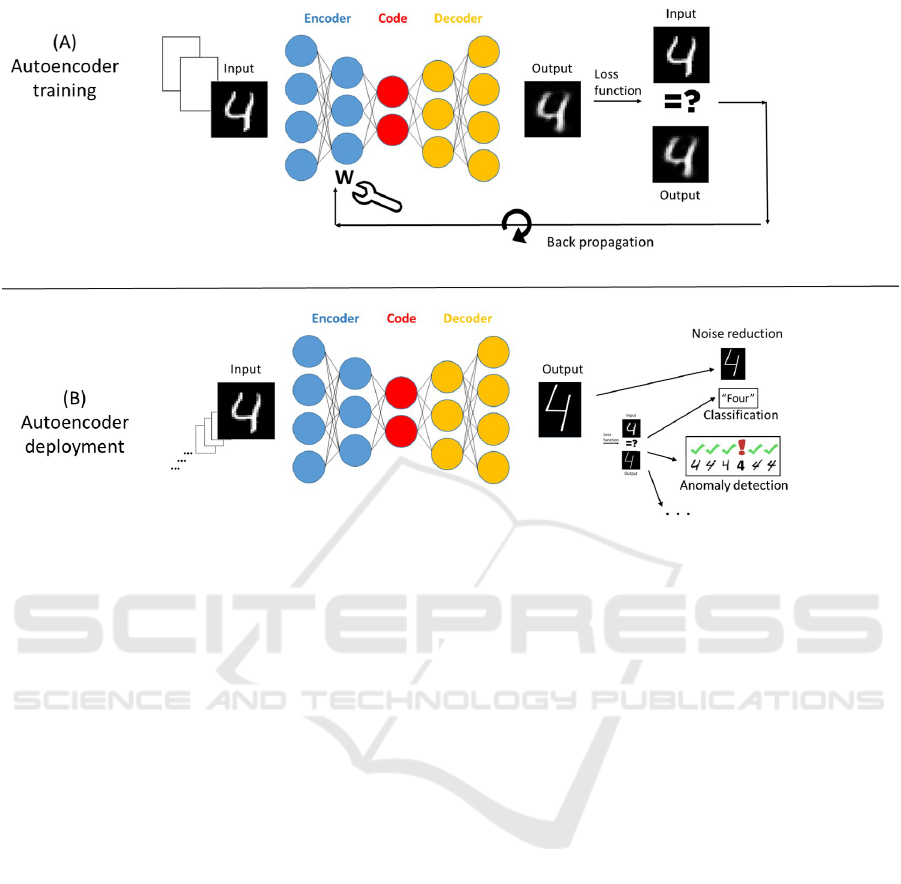
Figure 1: An autoencoder and autoencoding. The image and text are borrowed from (Cohen and Marron, 2022). See detailed

explanation in the text.

In Section 2, we provide some background infor-

mation about autoencoding. In Section 3, we describe

four groups of experiments that we have conducted

thus far, including the ML solution architecture and its

training and our assessment of the results. We plan to

continue our research and expand this initial set of ex-

periments. In Section 4, we document several conclu-

sions that shed light on this particular autoencoding

problem and the role of autoencoding in automated

modeling in general.

2 AUTOENCODERS AND

AUTOENCODING: OVERVIEW

Whether for understanding the results of scientiﬁc

observations in nature, extracting value from data

repositories, or enabling autonomous computer pro-

cessing, there is a growing need for automating the

discovery of the deﬁning features of individuals in

a given population. Once these features are estab-

lished, they can form a vector F = [ f

, f

,..., f

], such

that each individual x in the population can be repre-

sented sufﬁciently for the relevant use by an assign-

ment of a speciﬁc value v

to each feature f

; that is

x = [v

,...,v

Methods and tools for these purposes, under the

headings of feature extraction, dimensionality reduc-

tion, and autoencoding, range from principal compo-

nent analysis (PCA) to deep learning tools (Zhong

et al., 2016). A common ML approach is an AE (Bank

et al., 2020) — an unsupervised neural network model

designed to learn a meaningful representation of the

input data. This is done by learning how to encode

the inputs in the given population in such a way as to

make it possible to faithfully reconstruct them.

More speciﬁcally, Figure 1, borrowed from (Co-

hen and Marron, 2022) with some edits and clari-

ﬁcations, illustrates the concepts of an AE and au-

toencoding. Typical AEs include three network-based

elements: the encoder (blue circles), the code (also

termed the bottleneck layer, red circles), and the de-

coder (orange circles). The designer deﬁnes the archi-

tecture, activation functions, and initial weights of the

neural networks. Individual inputs (in this example,

handwritten digits) are fed into the encoder, encoded

as values in the code layer, and then reconstructed by

the decoder.

During training (A), a loss function computes the

differences between the output and the input. An op-

timization process then adjusts the weights W of the

edges connecting the neurons in order to minimize

this reconstruction loss. Training consists of numer-

ous repetitions using a ﬁnite set of examples.

Once training is complete, the AE is ready for de-

ployment (B) to perform its application task. Typical

applications include image search, cleaning out im-

MODELSWARD 2023 - 11th International Conference on Model-Based Software and Systems Engineering

276

age data by removing insigniﬁcant “noise”, anomaly

detection, classiﬁcation, and more. Encoding and de-

coding are then carried out with a ﬁxed encoder and

decoder: the initial neural net with the edge weights

determined in the training phase. The AE can now

process an unbounded number of inputs from the do-

main of interest.

We deﬁne autoencoding as the training process

described above. Autoencoding establishes a process

that can create a compact representation for every en-

tity in the input population. While the term autoen-

coding is used in practice, we have yet to ﬁnd an ex-

plicit deﬁnition for it. Hence we deﬁne it here, clar-

ifying that what we have in mind when we use the

term is the shaping of an encoder and a decoder dur-

ing training and not the encoding and decoding that

is carried out once the trained AE is deployed for its

application.

An AE with one fully-connected hidden layer, a

linear activation function, and a squared error loss

function is closely related to PCA (Plaut, 2018).

However, PCA is limited to encoding by only linear

transformations, where AEs based on neural nets can

employ nonlinear functions.

3 EXPERIMENTS

3.1 The Task: Autoencoding Line

Segments

As stated above, we wish to automatically discover

succinct representations for individuals in a popula-

tion of images, each containing one straight ﬁnite line

connecting two points. A computer program draws

the images in black-and-white in a prespeciﬁed res-

olution. This is a compromise between the abstract

concept of a line segment which has no color attribute

and whose width is zero, and an image of a real ob-

ject.

3.1.1 Inputs

In the experiments documented here, all images are

32 × 32 pixels (Autoencoding of handwritten digits is

often demonstrated using the MNIST dataset images

with 28 × 28 pixels). The training and validation set

consist of 15,000 and 1,000 images, respectively. The

process that creates each training and validation im-

age randomly chooses two pairs of coordinates and

draws the line connecting them using Bresenham’s

rasterizing algorithm.

3.1.2 Outputs and Loss Function

We modeled the task as a multi-label classiﬁcation

where each of the 32 × 32 output neurons holds the

probability that the corresponding pixel is 1. When

displaying the output, the grey level reﬂects this prob-

ability. We then had to deal with the problem of low

foreground-to-background ratio: the model can lower

the loss by reducing the error in the dominant easy-to-

classify background pixels rather than improving its

predictions for the foreground pixels. For example,

blank output images would have a relatively low loss

value. To handle this, we used Binary Focal Cross-

Entropy (Lin et al., 2017). For each pixel, we com-

puted

ℓ =

(

−α(1 − p)

log(p) if y = 1

−αp

log(1 − p) if y = 0,

(1)

where y is input pixel value, p ∈ [0,1] is the output

probability, γ is the focusing parameter and α is a

scaling parameter. This is a generalization of the stan-

dard Binary Cross-entropy function by introducing a

new term. For both cases in Eq. (1), the new term re-

duces the contribution of small errors (when the pre-

dicted probability is close to the correct value) to the

total result of the loss function. Thus, it reduces the

dominance of easy-to-classify background pixels in

the loss gradient. For all models, we used γ = 2 and

α = 0.25.

3.1.3 Role of Domain Knowledge

All models reﬂect in some way domain knowledge.

For example, all models include Convolutional Neu-

ral Network (CNN) layers. A set of neurons in a CNN

layer share the same weight set. Each one is con-

nected to a limited number of speciﬁc adjacent out-

put units in the previous layer, resulting in a convo-

lutional ﬁlter operating on its input. Simply put, the

model “knows” to look for spatial patterns in an or-

ganized input grid. However, this knowledge is lever-

aged only partly: the loss function treats each output

pixel independently of the others.

3.1.4 Experimentation Heuristics

In conducting these four groups of experiments (each

of which we described with one concrete case), we

did not follow a strict methodology. After building

an initial model in each approach, we adjusted the

hyperparameters until the incremental improvements

became very small. We then switched to a new ap-

proach. The criteria for analyzing and comparing re-

sults are discussed in the individual experiment de-

scriptions and in the conclusion section.

Toward Automated Modeling of Abstract Concepts and Natural Phenomena: Autoencoding Straight Lines

277

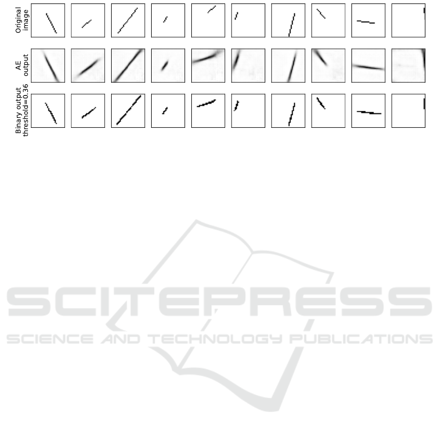
Figure 2: Results of AE1: a plain sequential AE. See the explanation in the text.

3.2 AE1: Plain Sequential Autoencoder

The architecture of AE1 is as follows. The bottleneck

layer, i.e., the code , is set to 4 neurons. The encoder

consists of 5 CNN layers followed by a single Fully

Connected (FC) layer. The number of ﬁlters in the

encoder CNN layers increases from one layer to the

next while the dimension of the output feature maps

decreases (using max pooling). The decoder consists

of the transposed architecture.

Figure 2 shows the results of AE1 with the ﬁrst ten

validation set images, illustrating the handling of dif-

ferent lengths, angles, and locations within the image.

The model certainty is high in the line’s middle sec-

tion for all raw outputs: narrow and dark. However,

near the line ends, the pixels are spread and are greyer,

indicating a lower certainty. Applying a threshold of

0.36 to all pixels reveals clearer images (bottom row),

most of which approximate the input to some degree.

All lines share the same “step” pattern for diag-

onal sections except for the rightmost image, where

the original diagonal line is reconstructed as a straight

vertical line. It will be interesting to explore whether

there is value in capturing in a loss function this sen-

sitivity of humans, where the difference between (in

this case) “zero steps” and “one step” draws our at-

tention more than the difference between, say, “ten

steps” and “eleven steps”. Note also that all lines are

thicker than the input ones, and some do not have the

same length and angle as the input (e.g., the ﬁfth im-

age from the left).

3.3 AE2: Customizing the Encoder

Using Domain Knowledge

An intuitive way for humans to represent a line is by

capturing the coordinates of its two ends. Given such

encoding, decoding would mean to “just” draw a line

from one end to the other (however, this decoding by

drawing a line is not a trivial task for a neural net).

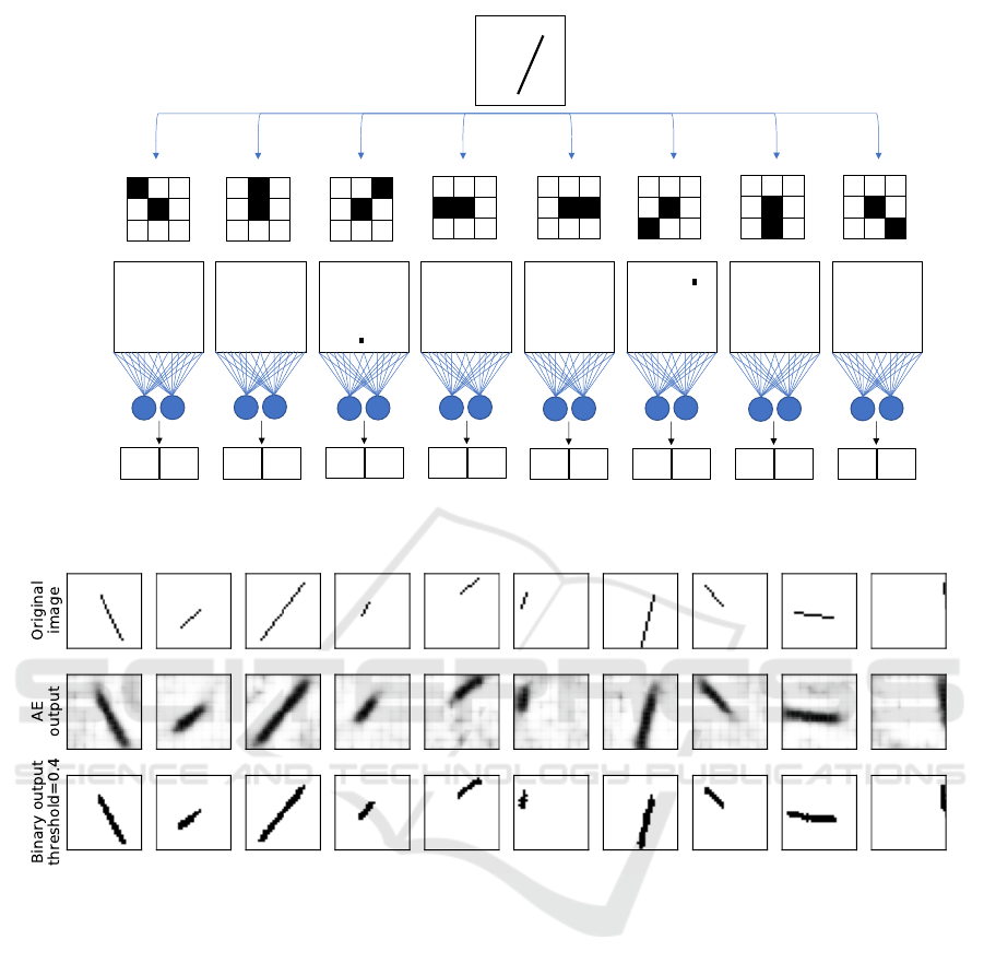
As shown in Fig. 3, the encoder looks separately

for the eight possible conﬁgurations of line ends, re-

lying on the domain knowledge/assumption that when

rasterizing the thinnest possible line, Bresenham’s al-

gorithm does not create an L-shaped arrangement of

black pixels. Exactly two of these conﬁgurations will

be found, yielding a feature map with a positive value

at the respective locations. The other six feature maps

will be all zeros. Ultimately, the encoder translates

each feature map into a pair of numbers. For example,

the third feature map from the left captures the bottom

end of the line, and the pair of neurons record its loca-

tion in the 32× 32 image ([15, 27]). The encoder then

concatenates the result into a 16-neuron sparse bottle-

neck layer (in a sparse code layer, for any given input,

only a small portion of the neurons contains non-zero

values). The decoder consists of eight sequential FC

layers and two CNN-transposed layers.

All the output images of AE2 have a gray back-

ground (Fig. 4); the lines are thicker than the in-

put. Some short lines and lines located near the image

boundaries appear as blotches (fourth and sixth from

the left and the rightmost outputs). Applying a binary

threshold (this time with a value of 0.4) “cleans” the

background and sharpens some lines, but some im-

ages do not seem like lines.

3.4 AE3: Customizing the Loss

Function Using Domain Knowledge

The customization of AE3 is between the extremes

of AE1 and AE2. AE1 has a plain architecture with a

relatively large number of parameters and without any

heuristics in the optimization of image reconstruction.

By contrast, AE2 uses ﬁxed prespeciﬁed CNN ﬁlters

in a specially designed encoder. In AE3, the encoder

and decoder are the same as in AE1. In addition, using

the same technique as in AE2, we add to the decoder a

MODELSWARD 2023 - 11th International Conference on Model-Based Software and Systems Engineering

278

Filters

Original image

Filters

Outputs

y x

2 FC

neurons

per filter

output

0 0 0 0

15 27 0 0

0 0 26 9

0 0 0 0

Latent

code

Figure 3: The encoder of AE2. It employs the 8 CNN ﬁlters to capture any line end conﬁguration. See the explanation in the

text.

Figure 4: Results of AE2. See the explanation in the text.

component that detects line end locations in the input

images and returns the corresponding reconstructed

pixel values as additional information that is then used

by the loss function.

Figure 5 depicts the results of AE3 on the same

ﬁrst ten validation set images. AE3 emphasizes pix-

els at the ends of the output lines. In most images in

the validation set, the rest of the output line is thin,

reﬂecting a satisfactory reconstruction. However, the

intensity is lower than at the line ends, suggesting that

the AE lacks conﬁdence in this prediction. In addi-

tion, several results are similar to AE2’s: short lines

and lines near the image boundary appear as blotches,

not as lines (for example, the fourth and sixth from

the left). For a small group of lines with edges at

the boundaries, the output image was completely dis-

torted (not shown).

3.5 AE4: a Variational Autoencoder

A variational autoencoder (VAE) (Kingma and

Welling, 2013; Doersch, 2016) is different from clas-

sic AEs in that (i) all the code vectors for a given

population are forced to occupy a continuous sub-

space with a normal distribution; (ii) implied by the

above: the model is generative—if an arbitrary code

value that falls within the code subspace is fed to the

decoder, the output entity is a valid instance of the

population; (iii) as part of forcing the code space to

be continuous, during encoding, the VAE samples the

code vector from a speciﬁc distribution; as a result,

the code vector for a given input may change between

runs.

The encoder of AE4 is composed of three sequen-

tial CNN layers, another FC layer, and two additional

FC “parallel” layers. Each of the two “parallel” FC

Toward Automated Modeling of Abstract Concepts and Natural Phenomena: Autoencoding Straight Lines

279

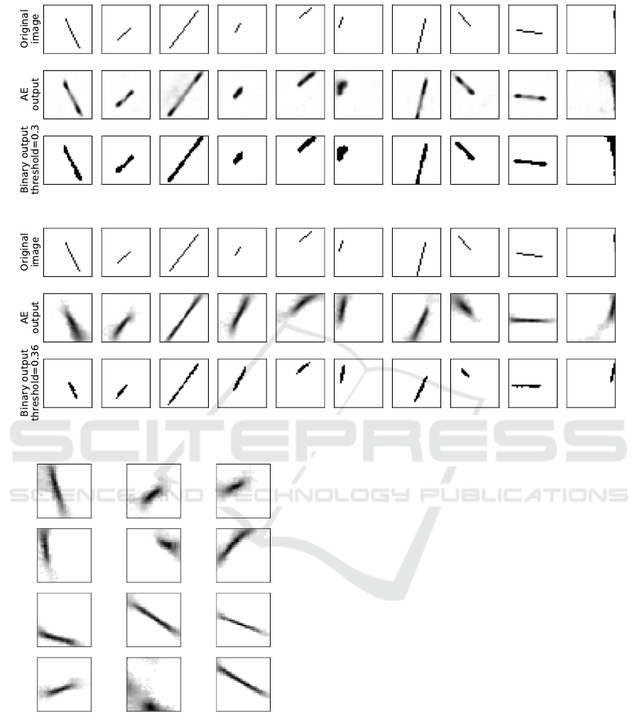
Figure 5: Results of AE3. See the text for details.

Figure 6: Results of AE4. See the explanation in the text.

Figure 7: AE4 line generation.

layers is separately connected to the last layer. The

two corresponding output vectors are mean and stan-

dard deviation vectors from which code vectors are

then sampled (using Gaussian distribution). The de-

coder consists of two sequential FC layers and three

CNN-transposed layers that output images.

Results are depicted in Fig. 6. The lines in the out-

put are broad, and many additional pixels appear with

a non-zero probability. Interestingly, in the rightmost

image, pixel intensity is relatively high in a region far

from the original position of the line (a gray blotch at

the bottom edge of the image). Figure 7 shows the re-

sults of twelve generated images using randomly sam-

pled vectors as code for the decoder. Roughly half

display the emergence of a straight line segment.

3.6 Code Interpretability

In automated modeling, naturally, one would be inter-

ested in intuitive codes that reﬂect how humans think

about and compare entities in the given population.

Thus, in the various experiments, we are working now

on interpreting the code pattern, checking if it results,

for example, in the pair of [x,y] coordinates or in other

intuitive codes as described in the introduction. In the

above examples, the code produced by AE2 is indeed

intuitive and explainable.

4 DISCUSSION & CONCLUSIONS

We draw from the above experiments the following

interim conclusions and open problems.

MODELSWARD 2023 - 11th International Conference on Model-Based Software and Systems Engineering

280

1. In this work, we presented four different AEs

for the task of autoencoding images of line seg-

ments. Though the results are all different, we

ﬁnd it challenging to measure them according to

well-speciﬁed criteria and then somehow com-

pose these measurements into a single numerical

grade. For example: AE1 yields thin lines with

moderate uncertainty regarding the edges. AE2

yields thick lines and struggles with short lines

or lines near the image borders. AE3 results in

relatively thin lines with high conﬁdence at the

edges but, again, has difﬁculty with lines that are

short or near the image frame. Lastly, AE4 yields

lines with signiﬁcant uncertainty in areas far from

the original line position. How does one translate

such critique into an order relation?

Loss function values cannot readily serve as this

ordering measure since some models use addi-

tional terms and some deviations that appear small

to the human eye turn out to produce large loss

values. For example, a reconstructed image of a

vertical line identical to the input but shifted by

one pixel to the right would result in a great loss

value, while a human observer may initially see

the two images as identical.

Moreover, with or without such measures of qual-

ity, it is difﬁcult to measure how much of an AE

result is due to domain knowledge (which simpli-

ﬁes the learning task), over-ﬁtting to the training

data, or superior general learning techniques.

2. In the ﬁeld of ML, autoencoding is referred to as

being unsupervised since inputs are not labeled.

We observe that the process involves many as-

pects of external control, including the choice of

the ML architecture, the loss function, and the in-

put representation for the real-world concept that

is to be autoencoded. Furthermore, learning a

concept may require knowledge of and assump-

tions about other concepts, as in the reliance on

understanding endpoints in some of our experi-

ments. Recall that such a-priori knowledge or as-

sumptions may also result in a bias in the ML pro-

cess itself.

We believe that methodologies for design of such

ML and AE solutions should include search-

ing for and documenting the reliance—explicit

or implicit—on external knowledge and assump-

tions. The goal is not necessarily to avoid such re-

liance altogether but to construct relevant ontolo-

gies that may dictate alternative orders for learn-

ing and autoencoding in a given domain.

3. In building a model based on observation and

sensing, each representation, like an image or an

audio or touch signal, extracts only a limited num-

ber of features of the real-world object. Modeling

all properties and interactions of a given object

type may require multiple representations or the

use of pre-existing domain knowledge. For ex-

ample, a unique property of a line segment, com-

pared to an arc or a line with multiple angles, is

its “straightness”. In a classical rectangular grid

of pixels arranged densely in ﬁxed locations, each

pixel is surrounded by exactly eight other pix-

els. The straightness of the line is not directly

represented; it has to be inferred from emergent

step patterns. An alternative image representation

could be ﬂoating sparse pixels whose location and

distance from each other are speciﬁed as numbers

with decimal precision that exceeds the resolution

of any standard pixel-based image. This approach

may represent straightness better, but the property

of the continuity of the line may have to be in-

ferred using other methods.

In summary, automated ontology acquisition will

likely require and contribute advances in algorithms

and techniques in ML, perception and knowledge

management.

5 FUTURE WORK

Our ongoing exploration and plans include dealing

with combinations of the following and more:

• Develop methodologies for measuring and com-

paring the quality of AE reconstructed outputs,

like (i) measuring the success of a human or pro-

gram in matching reconstructed outputs to the re-

spective inputs and (ii) measuring how close prop-

erties of the reconstructed output are to properties

of the corresponding real-world entity rather than

only to the (input) image of that entity.

• Investigate different adjustments to the loss func-

tion.

• Use higher resolution images with thicker and

smoother lines.

• Investigate additional domain-speciﬁc properties.

• Study interpretability of the resulting code.

ACKNOWLEDGEMENTS

We thank the anonymous reviewers for their com-

ments and suggestions. We thank Irun R. Cohen for

valuable discussions and insights. This work was par-

tially supported by research grants to David Harel

Toward Automated Modeling of Abstract Concepts and Natural Phenomena: Autoencoding Straight Lines

281

from the Estate of Harry Levine, the Estate of Avra-

ham Rothstein, Brenda Gruss and Daniel Hirsch, the

One8 Foundation, Rina Mayer, Maurice Levy, and

the Estate of Bernice Bernath, grant number 3698/21

from the ISF-NSFC joint to the Israel Science Foun-

dation and the National Science Foundation of China,

and a grant from the Minerva foundation.

REFERENCES

Bank, D., Koenigstein, N., and Giryes, R. (2020). Autoen-

coders. arXiv preprint arXiv:2003.05991.

Cohen, I. R. and Marron, A. (2022). The biosphere com-

putes evolution by autoencoding interacting organ-

isms into species and decoding species into ecosys-

tems. arXiv preprint arXiv:2203.11891.

Doersch, C. (2016). Tutorial on variational autoencoders.

arXiv preprint arXiv:1606.05908.

Fang, W., Ma, L., Love, P. E., Luo, H., Ding, L., and

Zhou, A. (2020). Knowledge graph for identifying

hazards on construction sites: Integrating computer

vision with ontology. Automation in Construction,

119:103310.

Kahani, N. (2018). Automodel: a domain-speciﬁc language

for automatic modeling of real-time embedded sys-

tems. In 2018 IEEE/ACM 40th International Con-

ference on Software Engineering: Companion (ICSE-

Companion), pages 515–517. IEEE.

Kingma, D. P. and Welling, M. (2013). Auto-encoding vari-

ational bayes. arXiv preprint arXiv:1312.6114.

Kochbati, T., Li, S., G

erard, S., and Mraidha, C. (2021).

From user stories to models: A machine learning em-

powered automation. In MODELSWARD, pages 28–

40.

Lin, T.-Y., Goyal, P., Girshick, R., He, K., and Doll

ar, P.

(2017). Focal loss for dense object detection. In

Proceedings of the IEEE international conference on

computer vision, pages 2980–2988.

Nardello, M., Han, S., Møller, C., and Gøtze, J. (2019). Au-

tomated modeling with abstraction for enterprise ar-

chitecture (ama4ea): business process model automa-

tion in an industry 4.0 laboratory. Complex Systems

Informatics and Modeling Quarterly, (19):42–59.

Plaut, E. (2018). From principal subspaces to principal

components with linear autoencoders. arXiv preprint

arXiv:1804.10253.

Tho, Q. T., Hui, S. C., Fong, A. C. M., and Cao, T. H.

(2006). Automatic fuzzy ontology generation for se-

mantic web. IEEE transactions on knowledge and

data engineering, 18(6):842–856.

Zhong, G., Wang, L.-N., Ling, X., and Dong, J. (2016). An

overview on data representation learning: From tra-

ditional feature learning to recent deep learning. The

Journal of Finance and Data Science, 2(4):265–278.

MODELSWARD 2023 - 11th International Conference on Model-Based Software and Systems Engineering

282