Managing Inventory Level and Bullwhip Effect in Multi Stage Supply

Chains with Perishable Goods: A New Distributed Model Predictive

Control Approach

Beatrice Ietto

1 a

and Valentina Orsini

2 b

DIMA, UNIVPM, Ancona, Italy

DII, UNIVPM, Ancona, Italy

Keywords:

Supply Chain Management, Inventory Control, Bullwhip Effect, Model Predictive Control.

Abstract:

We consider the inventory control problem for multi stage Supply Chains (SC) whose dynamics is character-

ized by uncertainties on the perishability factor of stocked goods and on the customer forecast information.

The control problem is to deﬁne a replenishment policy keeping the inventory level as close as possible to a

desired value and mitigating the Bullwhip Effect (BE). The solution we propose is based on Distributed Ro-

bust Model Predictive Control (DRMPC) approach. This implies solving a constrained min-max optimization

problem. To drastically reduce the numerical complexity of this problem, the control signal is parametrized

using B-spline functions.

1 INTRODUCTION

MPC techniques for multi stage SC are usually im-

plemented according to three different control archi-

tectures: centralized, decentralized and distributed.

The ﬁrst two are discussed in (Alessandri et al.,

2011),(Fu et al., 2014),(Fu et al., 2016),(Mestan et al.,

2016),(Perea-Lopez et al., 2003). The main limita-

tions of centralized approach are: numerical com-

plexity, computational cost, reluctance to share infor-

mation. Decentralized approach does not have these

drawbacks but causes a loss of performance because

control agents decide control actions independently

on each other. Thus, the interest has recently focused

on Distributed MPC (DMPC) (Fu et al., 2019),(Fu

et al., 2020),(Kohler et al., 2021).The above men-

tioned papers do not take into account the presence

of deteriorating items in the inventory system. On

the other hand, if the effect of perishable goods is not

taken into consideration, a serious degradation of the

supply chain system is observed. Centralized MPC of

inventory level for perishable goods has been inves-

tigated in (Hipolito et al., 2022; Lejarza and Baldea,

2020). These latter papers assume an exactly known

deteriorating factor. However, this simplifying as-

sumption is not satisﬁed in the overwhelming part of

practical cases (Chaudary et al., 2018).

https://orcid.org/0000-0001-5617-8228

https://orcid.org/0000-0003-4965-5262

Given the previous literature, the purpose of this

paper is to propose a DRMPC approach for the op-

timal inventory control of a multi stage SC with de-

teriorating items. Extending previous results on sin-

gle stage SC (Ietto and Orsini, 2022), our purpose

is to deﬁne a DRMPC policy optimally conciliating

the three following antagonist Control Requirements

(CR) at each stage: CR1) maximize the satisﬁed de-

mand issued by the neighboring downstream stage,

CR2) minimize the on hand stock level, CR3) miti-

gate the BE.

The ﬁrst step to face this problem is to deﬁne a

suitable predictive information on the end-customer

demand. In this paper we only assume that at any time

instant k ∈ Z

and over a ﬁnite prediction horizon, the

future end-customer demand entering the ﬁrst stage

of the SC is arbitrarily time varying inside a given

compact set D

1,k

. Coherently with this assumption

we conciliate CR1 and CR2 deﬁning a desired inven-

tory level that, for the ﬁrst stage of the SC, is given

by the upper bounding trajectory of D

1,k

. Then, the

target inventory level of each other upward stage is it-

eratively deﬁned on the basis of the predicted demand

coming from the previous downstream stage. Satis-

fying CR3 is a problem of a paramount importance in

the multi-stage SC management as testiﬁed by the im-

pressive amount of relevant literature, (Dejonckeere

et al., 2003),(Giard and Sali, 2013).

We face this problem simultaneously acting on

two Fundamental Features (FF) of BE.

Ietto, B. and Orsini, V.

Managing Inventory Level and Bullwhip Effect in Multi Stage Supply Chains with Perishable Goods: A New Distributed Model Predictive Control Approach.

DOI: 10.5220/0011885300003396

In Proceedings of the 12th International Conference on Operations Research and Enterprise Systems (ICORES 2023), pages 229-236

ISBN: 978-989-758-627-9; ISSN: 2184-4372

 2023 by SCITEPRESS – Science and Technology Publications, Lda. Under CC license (CC BY-NC-ND 4.0)

229

FF1) irregularity of stock replenishment orders,

FF2) progressive upward ampliﬁcation of the inter-

vals over which the replenishment orders issued by

each stage take values.

FF1 is addressed deﬁning a replenishment policy

parametrized in terms of smooth functions and deﬁn-

ing a cost functional penalizing excessive differences

between consecutive orders. As for FF2, we prove

that, using our approach, the upward interval ampli-

ﬁcation is proportional to the perishability rate. The

interesting corollary is that, in the case of non perish-

able goods, the values of orders issued by all stages

may be contained in the same ﬁxed amplitude inter-

val. Coherently with the assumptions on the uncer-

tainties and with the CR’s , we develop a DRMPC ap-

proach based on a min-max optimization procedure:

the control law is obtained minimizing the worst case

of a quadratic cost functional, which is computed by

maximizing with respect to all the possible perisha-

bility factor values. Another signiﬁcant novelty of

our approach is the parametrization of the replenish-

ment policy as a polynomial B-spline function. The

main reasons for this choice are: 1) polynomial B-

splines are smooth functions 2) B-splines are admit

a parsimonious parametric representation. given by a

time varying, linear, convex combination of some pa-

rameters named ”control points”. These properties al-

low us to obtain a replenishment order with a smooth

waveform and to transfer any hard constraint on the

control law to its control points. This is very use-

ful to deal with FF2 of BE. Property 2 also allows

us to reformulate the constrained minimization of the

cost functional with respect to the replenishment or-

der signal as a Weighted Constrained Robust Least

Square (WCRLS) estimation problem. that can be

efﬁciently solved using interior point methods (Lobo

et al., 1998).

2 PRELIMINARIES

2.1 B Splines Functions

A scalar, continuous time, B-spline curve is deﬁned

as a linear combination of polynomial basis functions

and control points, (De-Boor, 1978):

s(t) = B

(t)c, t ∈ [

ℓ+d+1

] ⊆ IR, (1)

where c = [c

,·· · , c

ℓ

]

and B

(t) =

1,d

(t),·· · , B

ℓ,d

(t)]. The c

’s are real numbers

representing the control points of s(t), the integer d is

the degree of the B-spline, the (

)

ℓ+d+1

i=1

are the non

decreasing knot points and the basis functions B

i,d

(t)

are computed by the Cox-de Boor recursion formula.

Remark 1. Eq. (1) shows that, once the degree d

and the knot points

have been ﬁxed, the scalar B

spline function s(t), t ∈ [

ℓ+d+1

], is completely de-

termined by the corresponding vector c of ℓ control

points.

2.2 The RLS Problem

Consider a set of linear equations D f ≈ b, with D ∈

r×m

, b ∈ IR

, m > r, subject to unknown bounded er-

rors: ∥δD∥ ≤ β and ∥δb∥ ≤ ξ (where the matrix norm

is the spectral norm). The RLS estimate

f ∈ IR

the value of f minimizing

min

max

∥δD∥≤β, ∥δb∥

≤

∥(D + δD) f − (b + δb)∥, (2)

In ((Lobo et al., 1998), p. 206), it is shown that prob-

lem (2) is equivalent to minimizing the following sum

of Euclidean norms

min

∥D f − b∥ + β∥ f ∥ + ξ (3)

Possible linear constraints on f can be taken into ac-

count imposing

f ≤ f ≤

f . (4)

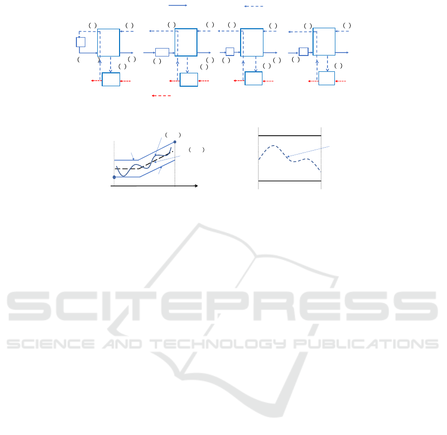
3 THE SYSTEM MODEL

As shown in Fig. 1, we consider an SC network con-

sisting of a cascade of stages (nodes) S

, i = 1,··· ,n,

characterized by counter-current order and material

streams. Management decisions for each node are

taken periodically at equally distributed time instants

kT where k ∈ Z

and T is the review period. At the

beginning of each review period [kT, (k + 1)T ) the

operations across the SC network are performed se-

quentially from S

to S

. Inside each review period,

each S

executes ﬁve actions in the following order:

receives delivery from supplier S

i+1

, logs the demand

of customer S

i−1

, measures its on hand stock level,

delivers the goods to meet demand and ﬁnally places

an order according to a suitably deﬁned replenishment

policy. Accordingly, ﬁve variables are deﬁned: s

(k),

(k), y

(k), h

(k) and u

(k). They represent the ship-

ment of goods from supplier S

i+1

, the demand from

i−1

, the on hand stock level, the delivery to customer

i−1

and the replenishment order, respectively. Each

node S

is regulated by an agent A

that solves a local

RMPC problem based on the following assumptions:

- A1) At any time instant k, and limitedly to an M

steps prediction horizon [k + 1,k + M

], the unknown

future end-customer demand d

(k + j), j = 1,·· · ,M

ﬂuctuates within a compact set D

1,k

limited below and

above by two known boundary trajectories: d

−

(k + j)

ICORES 2023 - 12th International Conference on Operations Research and Enterprise Systems

230

i+1

Order flow

Product flow

𝑈

!"#,%

𝑈

!,%

𝑈

&,%

𝐷

!"#,%

𝐷

&,%

…

ℎ

(𝑘)

𝑈

#,%

𝐷

!,%

𝐷

#,%

demand

𝑢

𝑘

ℎ

𝑘

𝑑

!"#

𝑘

𝑑

𝑘

𝑢

!"#

𝑘

𝑠

!"#

𝑘

ℎ

!"#

𝑘

𝑠

𝑘

𝑑

𝑘

𝑢

𝑘

ℎ

𝑘

…

𝑠

𝑘

…

i+1

…

𝑢

𝑘

𝑑

𝑘

i+1

forecast

demand

𝑦

𝑘

𝑦

𝑘

Information flow between agents

𝑦

!"#

𝑘

𝑦

𝑘

𝑠

𝑘 − L

Figure 1: Distributed control scheme of the n-subsystems SC network.

𝑑

# 𝑘 + 𝑗 , 𝑗 = 1, … , 𝑀

demand#forecast

𝑘 + 1

𝑘 + 𝑀

𝑑

(𝑘 + 𝑗)

𝑎

𝑏

𝑑

(𝑘 + 𝑗)

(𝑎)

the#end-customer#demand#

𝑑

𝑘 + 𝑗

𝑘 + 1

𝑘 + 𝑀𝑖

𝑢

!"#,%

𝑢

!"#,%

(𝑏)

𝑢

!"#

(k + l|k)

Figure 2: (a) Example of a set D

1,k

, (b) Example of a set D

i,k

, i > 1.

and d

(k + j), j = 1,·· · ,M

. The minimum value of

−

(k + j) and the maximum value of d

(k + j), j =

1,·· · ,M

, are denoted by d

−

1,k

and d

1,k

(points a and

b of Figure 2.(a) respectively). The demand forecast-

ing D

1,k

△

= [d

(k+1|k),··· ,d

(k+M

|k)] for agent A

is assumed to coincide with the central trajectory of

1,k

namely D

1,k

= [

(k + 1),··· ,

(k + M

)]. Fig-

ure 2.(a) shows a typical example of an end-customer

demand d

(k + j) and of a predicted end-customer de-

mand

(k + j) over a ﬁxed D

1,k

- A2) At any time instant k, the predicted demand

i,k

= [d

(k + 1|k),· ·· ,d

(k + M

|k)] for the other

agents A

, i = 2,··· ,n, coincides with the pre-

dicted optimal control sequence (i.e. the optimal

predicted replenishment policy U

i−1,k

△

= [u

i−1

(k +

1|k), · ·· ,u

i−1

(k + N

i−1

− 1|k)] transmitted by A

i−1

where M

= N

i−1

− 1. Note that also D

i,k

belongs

to a given compact set D

i,k

limited by the imposed

lower and upper values u

−

i−1,k

and u

i−1,k

respectively

(as shown in Fig. 2.(b)). How to compute U

i−1,k

−

i−1,k

and u

i−1,k

is explained in Section 4.

- A3) The goods shipped from supplier S

i+1

arrive

at customer S

with a time delay L

= n

T , where

∈ Z

. Goods arrive at customer S

new and de-

teriorate while kept in stock.

- A4) Inside each review period, the perishability rate

of the goods stocked in S

is α

∈ [α

−

,α

] ⊂ (0,1).

- A5) The operations of inventory replenishment and

goods delivery are executed simultaneously at the be-

ginning of each review period. Sales are not backo-

rdered.

The above assumptions imply that the stock level dy-

namics of the i-th node is described by the following

uncertain equation

(k + 1) = ρ

(k) + s

(k − L

) − h

(k)) (5)

where:

- y

(k) is the on hand stock level of S

, i.e. the amount

of goods left in stock after satisfying the demand at

the beginning of the k − 1 review period;

- s

(k − L

) is the goods delivered to the stage S

with

a time delay L

;

- the sum y

(k) + s

(k − L

) represents the effective

amount of goods available for sale at the beginning

of k-th review period;

- h

(k) is the demand fulﬁlled by S

, i = 1,· ·· ,n

(k)

△

= min{d

(k), y

(k) + s

(k − L

)} (6)

where d

(k) is the end-customer demand, d

(k) =

i−1

(k), i = 2,· · · ,n, is the demand issued by S

i−1

;

- ρ

△

= 1 − α

∈ [ρ

−

,ρ

] is the uncertain decay factor.

For future developments we now rewrite equation (5)

assuming A6): there exists a

k ≥ 0 such that

(k) + s

(k − L

) ≥ d

(k), ∀k ≥

k, i = 1,· ·· ,n (7)

By (6) and (7) we have h

i+1

(k) = d

i+1

(k). As

i+1

(k) = u

(k) and h

i+1

(k) = s

(k) (see Fig. 1) we

also have s

(k − L

) = u

(k − L

). Hence an equivalent

expression of (5) is

(k +1) = ρ

(k) +u

(k −L

)−h

(k)), ∀k ≥

k (8)

Assumption A6) is justiﬁed because, at each stage,

the control sequence is obtained minimizing the max-

imum weighted ℓ

norm of the distance between the

on-hand stock level and the maximum demand.

Managing Inventory Level and Bullwhip Effect in Multi Stage Supply Chains with Perishable Goods: A New Distributed Model Predictive

Control Approach

231

4 PROBLEM SETUP

To simplify the derivation of the control strategy we

refer to (8) in the ideal case

k = 0. Each A

uses

equation (8) and the predicted optimal control pol-

icy U

i−1,k

communicated by A

i−1

to predict the fu-

ture inventory level of the local subsystem S

. This

latter is in turn used to compute U

i,k

minimizing the

worst case of a local quadratic cost functional subject

to hard constraints u

−

i,k

and u

i,k

. Coordination between

contiguous agents A

i−1

and A

, is imposed by relat-

ing the respective constraints u

−

i−1

and u

i−1,k

with u

−

i,k

and u

i,k

. Each local RMPC requires each agent A

repeatedly solve a Min-Max Constrained Optimiza-

tion Problem (MMCOP) over a future N

steps control

horizon, and, according to the receding horizon con-

trol, to only apply the ﬁrst sample of the computed

predicted optimal control sequence.

4.1 Local MMCOP for A

The local MMCOP for any A

, i = 1,·· · ,n is formally

deﬁned as follows ∀k ∈ Z

min

(k|k),··· ,u

(k+N

−1|k)]

max

∈[ρ

−

,ρ

]

i,k

, (9)

−

i,k

≤ u

(k + j|k) ≤ u

i,k

, j = 0,· ·· ,N

− 1, (10)

where:

i,k

∑

l=1

(k + L

+ l)q

i,l

(k + L

+ l) +

∑

−1

l=1

i,l

∆u

(k + l|k) (11)

where e

(k + L

+ l) denotes the future values of the

tracking error given by

(k + L

+ l)

△

= r

(k + L

+ l) − y

(k + L

+ l) (12)

with

(k + L

+ l) = ρ

(k) +

−1

∑

ℓ=0

+l−ℓ

(k + ℓ − L

)

l−1

∑

ℓ=0

l−ℓ

(k + ℓ|k) −

+l−1

∑

ℓ=0

+l−ℓ

(k + ℓ). (13)

(k + L

+ l)

△







(k + L

+ l) i = 1

i−1,k

i = 2,· ·· ,n

(14)

and

∆u

(k + l|k)

△

= u

(k + l|k) − u

(k + l − 1|k) (15)

Remark 2. Some considerations on J

i,k

are now in or-

der.

-1) By A1), A2) and (14), it can be seen that M

≥

+ L

and M

= N

i−1

− 1 = N

+ L

, i > 1, namely

i−1

= N

+ L

+ 1.

-2) The time varying target inventory level r

(k) for S

is deﬁned as follows:

(k) = d

(k) and r

(k) = u

i−1,k

, i ≥ 2 (16)

For each ﬁxed k and over the corresponding predic-

tion interval [k,k + M

], i ≥ 2, deﬁnition (14) implies

that the values of the target inventory level are frozen

on u

i−1,k

. Keeping the on hand stock level as near

as possible to the possible maximum level of the de-

mand forecasting maximizes the amount of fulﬁlled

demand over each shifted prediction horizon and pre-

vents unnecessarily larger stock levels.

-3) The term

∑

−1

l=1

i,l

∆u

(k + l|k) and the way the

hard constraints (10) are deﬁned allow us to deal with

FF1 and FF2 respectively.

4.2 Determining u

−

i,k

and u

i,k

By CR1-CR3, the constraints on u

(k + j|k) imposed

by (10) are determined on the basis of the two follow-

ing criteria: 1) maximize the amount of demand sat-

isﬁed by each stage S

, 2) limit the amplitude (deﬁned

as A

i,k

) of the interval [u

−

i,k

]

△

= C

i,k

. We estimate

−

i,k

and u

i,k

with reference to two possible, limit sit-

uations compatible with (8). Consider the following

scenario:

-d

(k + L

+ j), j = 0,· · · ,N

− 1, is a constant sig-

nal with value

i,k

∈ [d

−

i,k

] = [u

−

i−1,k

]. The

two mentioned limit situations are

i,k

= u

−

i−1,k

and

i,k

= u

i−1,k

- Each control horizon H

i,k

is long enough to allow

(k + L

+ j), j = 1,··· ,N

, to practically attain the

steady-state value ˜y

i,k

under the forcing action of a

constant u

(k + j) = ˜u

i,k

, j = 0,·· · , N

− 1. The prob-

lem we now consider is: for a given constant demand

i,k

it is required to ﬁnd the interval C

i,k

where the

corresponding constant control input ˜u

i,k

takes values,

such that the resulting constant steady state state out-

put ˜y

i,k

satisﬁes ˜y

i,k

≥

i,k

, ∀ρ

∈ [ρ

−

,ρ

Some algebraic calculations (not reported for

brevity) based on z-transform methods and on the ﬁ-

nal value theorem (Kuo, 2007) show that

1,k

△

= [u

−

1,k

] =

−

1,k

] (17)

i,k

△

= [u

−

i,k

] =

−

i−1,k

,i = 2,·· · , n(18)

Recalling that A

i−1,k

denotes the amplitude of C

i−1,k

from (17),(18) we have

1,k

−

1,k

− d

−

1,k

),A

i,k

−

i−1,k

,i = 2···n (19)

ICORES 2023 - 12th International Conference on Operations Research and Enterprise Systems

232

To quantify the BE at node S

according to FF2 we

deﬁne the following measure:

i,k

i−1,k

(20)

According to (19)-(20), the proposed DRMPC

scheme implies B

i,k

= 1/ρ

−

△

= B

> 1.

The two salient conclusions are: 1) an estimate of

the overall BE (corresponding to FF2 ) which prop-

agates along the SC network, can be computed ”a

priori” and is given by B = 1/(

∏

i=1

−

), 2) our ap-

proach does not entail this kind of BE for ρ

−

→ 1.

5 REFORMULATION OF THE

MMCOP

We reformulate the local MMCOP as a WCRLS es-

timation to drastically reduce the numerical complex-

ity of the algorithm solving the original MMCOP. The

functional J

i,k

, deﬁned in (9), is minimized assuming

that the control sequence U

i,k

, is given by the sampled

version of a B-spline function. Adapting the notation

in (1) to specify that it is relative to the i-th node and

the k-th ﬁxed time instant we have

( j|k)

△

= B

i,d

( j)c

i,k

, j = k,··· ,k + N

− 1, (21)

with B

i,d

( j) = [B

i,1,d

( j),· ·· ,B

i,ℓ,d

( j)] and c

i,k

i,k,1

,·· · ,c

i,k,ℓ

]

. The parameter vector c

i,k

, deﬁning

( j|k), is computed as the solution of the WCRLS

estimation problem deﬁned beneath.

As ρ

∈ [ρ

−

], an equivalent representation of

is ρ

+ δρ

= (ρ

−

+ ρ

)/2 where

is the

nominal value and δρ

is the perturbation with respect

satisfying |δρ

| ≤ (ρ

− ρ

−

)/2. It follows that

= (

+ δρ

)

+ ∆ρ

i,k

(22)

where ∆ρ

i,k

△

= (

+ δρ

)

−

is the sum of all terms

containing δρ

in the explicit expression of (

δρ

)

. Analogously, by A1), A2), A6) and (6), the

future values h

(k + ℓ) in (13) can be expressed as

(k + ℓ) =

(k + ℓ|k) + δh

(k + ℓ|k) (23)

where

(k + ℓ|k) = d

(k + ℓ|k). Exploiting (21)-(23)

it can be shown that the future tracking error given by

(12) can be expressed as

(k + L

+l|k) = (b

i,k,l

+δb

i,k,l

)− (D

i,k,l

+δD

i,k,l

i,k

where

i,k,l

△

l−1

∑

ℓ=0

l−ℓ

i,d

(k + ℓ) (24)

δD

i,k,l

△

l−1

∑

ℓ=0

∆ρ

i,l−ℓ

i,d

(k + ℓ) (25)

i,k,l

△

= r

(k + L

+ l) −

(k)

−

−1

∑

ℓ=0

+l−ℓ

(k + ℓ − L

)

+l−1

∑

ℓ=0

+l−ℓ

(k + ℓ|k) (26)

δb

i,k,l

△

= −∆ρ

i,L

(k) −

−1

∑

ℓ=0

∆ρ

i,L

+l−ℓ

(k + ℓ − L

)

+l−1

∑

ℓ=0

+l−ℓ

δh

(k + ℓ|k) +

+l−1

∑

ℓ=0

∆ρ

i,L

+l−ℓ

(k + ℓ)

Similarly ∆u

(k +l|k) = b

i,k,l

−D

i,k,l

i,k

with D

i,k,l

−(B

i,d

(k + l) − B

i,d

(k + l − 1)) and b

i,k,l

= 0.

Deﬁning the following extended error vector

i,k







1/2

i,1

(k + L

+ 1)

1/2

i,N

−1

(k + L

+ N

− 1)

1/2

i,1

∆u

(k + 1|k)

1/2

i,N

−1

∆u

(k + N

− 1|k)







and the corresponding extended vectors b

i,k

, δb

i,k

and

matrices D

i,k

, δD

i,k

(not reported for brevity) allow

us to reformulate the local MMCOP (9)-(11) as the

following local WCRLS estimation problem:

min

i,k

max

∥δD

i,k

∥≤β

i,k

∥δb

i,k

∥≤ξ

i,k

∥e

i,k

∥

(27)

where

∥e

i,k

∥

= ∥(b

i,k

+ δb

i,k

) − (D

i,k

+ δD

i,k

∥

(28)

subject to u

−

i,k

≤ c

i,k,r

≤ u

i,k

,r = 1, ··· ,ℓ. (29)

It is seen that (28)-(29) deﬁne a problem of the

kind (2)-(4). Hence, according to Section 2.2, at any

k the local WCRLS estimation problem (27)-(29) can

be reformulated as

min

i,k

∥b

i,k

− D

i,k

∥ + β

i,k

∥c

i,k

∥ + ξ

i,k

(30)

where the components of c

i,k

must satisfy (29).

Remark 3. Note that ξ

i,k

of (30) is independent of c

i,k

so that it can be removed from the objective function.

This implies that in (30) only the upper bound β

i,k

on ∥δD

i,k

∥ needs to be determined at each k. More-

over the way the B-spline basis functions are deﬁned

by the Cox de Boor formula (De-Boor, 1978) implies

that B

i,d

(τ) = B

i,d

(τ + N

), ∀τ ∈ H

i,k

, k ∈ Z

. Hence,

by (25), one has that β

i,k

△

= β

, ∀k = 0,1,·· · and more-

over β

is can be determined putting ρ

= ρ

Managing Inventory Level and Bullwhip Effect in Multi Stage Supply Chains with Perishable Goods: A New Distributed Model Predictive

Control Approach

233

Feasibility and stability properties of the proposed

control strategy can be now formally stated in the fol-

lowing theorem (whose proof is omitted for brevity).

Theorem The proposed DRMPC strategy guaran-

tees the feasibility of each local MMCOP, the pos-

itivity of all physical variables u

(k) and y

(k), i =

1,·· · ,n, and their uniform boundedness.

6 NUMERICAL RESULTS

In this section, we perform simulated experiments on

the application of the proposed RDMPC to the man-

agement of an uncertain SC composed of n = 3 stages

, i = 1, ··· ,3, (retailer-distributor-factory). We as-

sume that the equations describing the stock level

dynamics of each S

are characterized by the same

perishability factor α

, time delay L

and initial state

(0). The model parameters of each S

are reported

in Table 1. At each k, the unknown future end-

customer demand d

(k), belongs to a known compact

set D

1,k

, with M

= 24. Figure 3 shows the actual

end-customer demand enclosed in the contiguous po-

sitioning of all the D

1,k

’s. The dashed red trajectory

is the predicted end-customer demand d

(k +l|k). We

use B-spline functions of degree d = 3 with ℓ = 6 con-

trol points over each control horizon H

i,k

. The other

tuning parameters of the local MMCOP for any A

i = 1,2, 3 are reported in Table 2.

0 50 100 150 200 250

Figure 3: The end-customer demand d

(k) and the two

boundary trajectories d

(k) and d

−

(k).

We evaluate the effectiveness of the proposed

method by deﬁning performance indicators that take

into account the ability to satisfy the demand at

each stage, to limit the inventory level and to re-

duce the BE. The ﬁrst performance indicator, that we

deﬁne, measures the normalized amount of Unsatis-

ﬁed Demand at each stage and is given by UD

△

∑

k=0

(k)

∑

k=0

(k) − h

(k)| ∈ [0 1], i = 1,2,3, where

is the length of the simulation. The second per-

formance indicator is the total sum of the Inventory

Stock in the SC after satisfying the demand at each

k = 0, ··· ,T

. In accordance with (5), it is given

by I S

△

∑

i=1

∑

k=0

(k). As for the BE, we de-

ﬁne a second performance indicator according to FF1:

∆u,i

∑

−1

k=0

(k + 1) − u

(k)|, i = 1, ··· ,n. It

measures ”a posteriori” the smoothness property of

each replenishment order u

(k), i = 1, ··· ,n. The sim-

ulation has been performed choosing ρ

= 0.885, i =

1,2,3 and it has been stopped at time k = 200 (namely

= 200). The generated orders u

(k), i = 1,2,3 are

displayed on the left hand side of ﬁgure 4. This ﬁg-

ure shows the ordering signal issued by each stage S

i = 1,2,3 with the respective time-varying lower and

upper bounds. The resulting inventory level y

(k) and

the time varying desired inventory level r

(k) for each

, i = 1,2,3 are reported on the left hand side of ﬁg-

ure 5. The imposed and fulﬁlled demands d

(k) and

(k) respectively at each S

are displayed on the left

hand side of ﬁgure 6.

A comparison has been performed with the

DTCM proposed in (Ignaciuk, 2013) where equations

(34),(35) have ben adapted to the case of an n-stage

SC with n = 3, uncertain decay factors ρ

∈ [0.86, 0.9]

and known time delays L

= 4, i = 1, 2, 3 obtaining

(k) = sat[ω

(k)] = sat[y

re f ,i

− PIP

(k)] (31)

where PIP

(k) = ρ

(k) +

∑

k−1

j=0

k− j

( j) −

∑

k−L

−1

j=0

k− j

( j) and the saturation function

sat(ω

)

△

= {ω

if ω

∈ [0,u

max,i

]; 0 if ω

0; u

max,i

if ω

> u

max,i

}. According to (45),(46) in

(Ignaciuk, 2013), u

max,i

and y

re f ,i

are inferiorly lim-

ited as: u

max,i

> d

max,i

and y

re f ,i

> d

max,i

∑

j=0

The topology of the SC network shown in ﬁgure 1 is

such that: d

max,1

= max

(k) and d

max,i

= u

max,i−1

i = 2, 3. The modiﬁed DTCM (31) has been applied

choosing: ρ

= 0.88, i = 1,2, 3, d

max,1

= 40,

max,1

= 45 > d

max,1

, u

max,2

= 50 > d

max,2

= 45,

max,3

= 55 > d

max,3

= 50, y

re f ,1

= 160 > 157,

re f ,2

= 180 > 177 and y

re f ,3

= 200 > 196.

The orders u

(k) generated (with ρ

= 0.88) and

the resulting on hand stock level y

(k) (generated

with ρ

= 0.885) are reported on the right hand side

of ﬁgures 4 and 5 respectively.

The performance evaluation of both methods is

performed on the basis of the performance indicators

previously deﬁned. The results are summarized in

table 3. Both methods fully satisfy the end-customer

demand d

(k) (as numerically quantiﬁed by the

performance indicator UD

reported in table 3)

but the DRMPC approach requires a very smaller

warehouse occupancy with respect to DTCM. This

is visually evidenced by ﬁgure 5 and numerically

quantiﬁed by I S (see table 3). The reduction of

warehouse occupancy is a consequence of tracking a

time varying inventory level r

(k) which is adapted

ICORES 2023 - 12th International Conference on Operations Research and Enterprise Systems

234

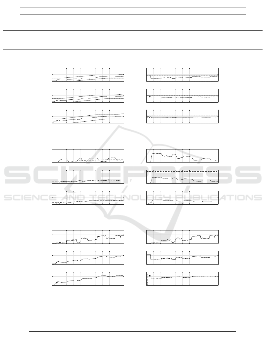
Table 1: Parameters of each node S

, i = 1, 2,3.

time delay perishability factor decay factor initial state

= 4 α

∈ [α

−

,α

] = [0.1,0.14] ρ

= 1 − α

∈ [ρ

−

,ρ

] = [0.86,0.9] y

(0) = 0

Table 2: Tuning parameters of the local MMCOP for any A

, i = 1, 2,3.

length of each H

i,k

scalar weights in (11) the scalars β

i,k

△

= β

in (30)

= M

− L

△

= N

i−1

− (L

+ 1) i > 1 q

i,l

= 20 N

= 15 N

= 10 e

−0.1 (l−1)

−1 (l−1)

= 1.88 β

= 1.38 β

= 0.89

0 20 40 60 80 100 120 140 160 180 200

100

S1: the boundary trajectories (dotted) and the ordering signal u

(k)

0 20 40 60 80 100 120 140 160 180 200

100

S2: the boundary trajectories (dotted) and the ordering signal u

(k)

0 20 40 60 80 100 120 140 160 180 200

(DRMPC)

100

S3: the boundary trajectories (dotted) and the ordering signal u

(k)

0 20 40 60 80 100 120 140 160 180 200

100

S1: the boundary trajectories (dotted) and the ordering signal u

(k)

0 20 40 60 80 100 120 140 160 180 200

100

S2: the boundary trajectories (dotted) and the ordering signal u

(k)

0 20 40 60 80 100 120 140 160 180 200

(DTCM)

100

S3: the boundary trajectories (dotted) and the ordering signal u

(k)

Figure 4: Comparison (DRMPC)-(DTCM): the ordering signal u

(k) issued by each S

0 20 40 60 80 100 120 140 160 180 200

100

200

S1: the desired reference r

(k)(dashed) and the on hand stock level y

(k) (solid)

0 20 40 60 80 100 120 140 160 180 200

100

200

S2: the desired reference r

(k) (dashed) and the on hand stock level y

(k) (solid)

0 20 40 60 80 100 120 140 160 180 200

(DRMPC)

100

200

S3: the desired reference r

(k) (dashed) and the on hand stock level y

(k) (solid)

0 20 40 60 80 100 120 140 160 180 200

100

200

S1: the desired reference r

(k)=160 (dashed) and the on hand stock level y

(k) (solid)

0 20 40 60 80 100 120 140 160 180 200

100

200

S2: the desired reference r

(k)=180 (dashed) and the on hand stock level y

(k) (solid)

0 20 40 60 80 100 120 140 160 180 200

(DTCM)

100

200

S3: the desired reference r

(k)=200 (dashed) and the on hand stock level y

(k) (solid)

Figure 5: Comparison (DRMPC)-(DTCM): the desired inventory level r

(k) and the on hand stock level y

(k) of each S

0 20 40 60 80 100 120 140 160 180 200

S1: the satisfied demand v

(k)(dashed) and the imposed demand d

(k) (solid)

0 20 40 60 80 100 120 140 160 180 200

S2: the satisfied demand v

(k) (dashed) and the imposed demand d

(k)=u

(k) (solid)

0 20 40 60 80 100 120 140 160 180 200

(DRMPC)

S3: the satisfied demand v

(k) (dashed) and the imposed demand d

(k)=u

(k) (solid)

0 20 40 60 80 100 120 140 160 180 200

S1: the satisfied demand v

(k)(dashed) and the imposed demand d

(k) (solid)

0 20 40 60 80 100 120 140 160 180 200

S2: the satisfied demand v

(k) (dashed) and the imposed demand d

(k)=u

(k) (solid)

0 20 40 60 80 100 120 140 160 180 200

(DTCM)

S3: the satisfied demand v

(k) (dashed) and the imposed demand d

(k)=u

(k) (solid)

Figure 6: Comparison (DRMPC)-(DTCM): the imposed demand d

(k) and the fulﬁlled demand h

(k) at each S

Table 3: The performance evaluation of the DRMPC and DTCM strategies.

I S BE

∆u,1

∆u,2

∆u,3

DRMPC 0 0.0089 0.004 2.1894 × 10

74.3 92 106.8

DTCM 0 0.0526 0.0201 3.4895 × 10

232.4 152 108.7

at any k on the basis of the current demand d

(k).

On the contrary DTCM deﬁnes a constant desired

inventory level y

re f ,i

for each S

, which is ”a priori”

computed using a conservative formula requiring the

Managing Inventory Level and Bullwhip Effect in Multi Stage Supply Chains with Perishable Goods: A New Distributed Model Predictive

Control Approach

235

”a priori” knowledge of the maximum value d

max,1

the end-customer demand over an indeﬁnitely long

future time interval. Moreover, as d

max,1

is never

exactly known, it is often over-estimated.

The diagrams displayed in ﬁgure 4 and the entries

of columns 5-7 of table 3 show that the DRMPC pol-

icy provides a smoother control signal with respect

to the DTCM strategy. Moreover ﬁgure 4 evidences

how the interval containing each replenishment order

(k) is tighter in the DRMPC strategy. Our approach

is able to limit the amplitude of such intervals and

consequently to strictly control the FF2 of BE.

7 CONCLUSIONS

The main novelties we propose in this paper are: 1)

the supply chain dynamics is characterized by per-

ishable goods with uncertain decay factor, 2) the

proposed DRMPC approach provides a B-splines

parametrization of the replenishment order. The

B-splines parametrization allows us to reformulate

the min-max optimization problem implied by the

DRMPC as a simpler WCRLS estimation problem.

The method we propose also allows us to deﬁne a

time-varying inventory level conciliating the opposite

control requirements CR1 and CR2. CR3 is addressed

penalizing the difference between control moves and

also parametrizing the control moves as polynomial

B-spline functions. The numerical test conﬁrms the

validity of the approach: it is actually able to reduce

the inventory level without affecting customer service

quality and without incurring an excessive control ef-

fort.

REFERENCES

Alessandri, A., Gaggero, M., and Tonelli, F. (2011). Min-

max and predictive control for the management of dis-

tribution in supply chains. IEEE Transactions on Con-

trol System Technology, 19:1075–1089.

Chaudary, V., Kulshrestha, R., and Routroy, S. (2018). State

of the art literature review on inventory models for

perishable products. Journal of Advances in Manage-

ment Research, 1:306–346.

De-Boor, C. (1978). A practical guide to splines. Springer

Verlag, New York, 2nd edition.

Dejonckeere, J., Disney, S., Lambrecht, M., and Towill, D.

(2003). Measuring and avoiding the bullwhip effect: a

control theoretic approach. European Journal of Op-

erational Research, 147:567–590.

Fu, D., Ionescu, C., Aghezzaf, E., and Kayser, R. D. (2014).

Decentralized and centralized model predictive con-

trol to reduce the bullwhip effect in supply chain

management. Computers & Industrial Engineering,

73:21–31.

Fu, D., Ionescu, C. M., Aghezzaf, E., and Kayser, R. D.

(2016). A constrained epsac to inventory control for a

benchmark supply chain system. International Jour-

nal of Production Research, 54:232–250.

Fu, D., Zhang, H., Dutta, A., and Chen, G. (2020). A coop-

erative distributed model predictive control approach

to supply chain management. IEEE Transactions on

Systems Man and Cybernetics, 50:4894–4904.

Fu, D., Zhang, H., Ionescu, C. M., Aghezzaf, E., and

Kayser, R. D. (2019). A distributed model predictive

control strategy for the bullwhip reducing inventory

management policy. IEEE Transactions on Industrial

Informatics, 15:932–941.

Giard, V. and Sali, M. (2013). The bullwhip effect in supply

chains: a study of contingent and incomplete litera-

ture. International Journal of Production Economics,

51:3380–3893.

Hipolito, T., Nabais, J., Benitez, R., Botto, M., and Negen-

born, R. (2022). A centralised model predictive con-

trol framework for logistics management of coordi-

nated supply chain of perishable goods. International

Journal of Systems Science: Operation & Logistics,

9:1–21.

Ietto, B. and Orsini, V. (2022). Resilient robust model

predictive control of inventory systems for perish-

able good under uncertain forecast information. In

2022 International Conference on Cyber-physical So-

cial Intelligence (Best paper ﬁnalists award). IEEE.

Ignaciuk, P. (2013). Discrete inventory control in systems

with perishable goods- a time delay system perspec-

tive. IET Control Theory and Applications, 8:11–21.

Kohler, P., Muller, M., Pannek, J., and Allgower, F. (2021).

Distributed economic model predictive control for co-

operative supply chain management using customer

forecast information. IFAC Journal of Systems and

Control, 15:1–14.

Kuo, B. (2007). Digital Control Systems. Oxford University

Press, Oxford, 2nd edition.

Lejarza, F. and Baldea, M. (2020). Closed-loop real-time

supply chain management for perishable products.

IFAC PapersOnLine, 53:11458–14463.

Lobo, M., Vandenberghe, L., Boyd, S., and L

ebret, H.

(1998). Second-order cone programming. Linear Al-

gebra and its Applications, 284:193–218.

Mestan, E., Metin, M. T., and Arkun, Y. (2016). Optimiza-

tion of operations in supply chain systems using hy-

brid systems approach and model predictive control.

Ind. Eng. Chem, 45:6493–6503.

Perea-Lopez, E., Ydstie, B., and Grossmann, I. (2003). A

model predictive control strategy for supply chain op-

timization. Computers and Chemical Engineering,

27:1201–1218.

ICORES 2023 - 12th International Conference on Operations Research and Enterprise Systems

236