Data Augmentation, Multimodality, Subject and Activity Speciﬁcity

Improve Wearable Electrocardiogram Denoising with Autoencoders

ao Areias Saraiva

1,2,3 a

, Mariana Abreu

1,3 b

, Ana Soﬁa Carmo

1,3 c

, Ana Fred

1,3 d

and Hugo Pl

acido da Silva

1,3 e

Department of Bioengineering, Instituto Superior T

ecnico, Univeristy of Lisbon, Portugal

Department of Computer Science and Engineering, Instituto Superior T

ecnico, Univeristy of Lisbon, Portugal

Pattern and Image Analysis Group, Instituto de Telecomunicac¸

oes, Portugal

Keywords:

Biosignal Denoising, Electrocardiogram, Accelerometry, Ambulatory Wearables, Data Augmentation.

Abstract:

Event detection based on biosignals continuously acquired by wearable devices has become an emergent

topic. Particularly, real-time event detection with the electrocardiogram (ECG) has been explored to monitor

heart conditions and epileptic seizures in the ambulatory. However, ECG acquired in the ambulatory is much

more prone to noise and artifacts, due to the dynamic nature of these environments. Therefore, real-time and

robust ECG denoising methods are crucial if event detection is meant to succeed. Denoising autoencoders

(DAEs) are studied as robust and fast methods to attenuate ECG noise and artifacts. ECG data augmentation

techniques are shown to effectively improve the performance of such a deep learning method. Activity and

subject speciﬁc models are shown to output better ECG denoised estimates, than non-speciﬁc ones. And using

accelerometry (ACC) as noise reference exempliﬁes how biosignal multimodality improves ECG attenuation

of muscle and motion artifacts. Therefore, this work establishes effective design techniques to be considered

when engineering ECG deep learning models.

1 INTRODUCTION

Portable electrocardiography for the ambulatory is

currently a necessity to monitor patients outside the

hospital (Bansal and Joshi, 2018; Bayoumy et al.,

2021). At the same time, automation of that moni-

toring has become an emerging topic (Prieto-Avalos

et al., 2022), since human professional monitoring

is infeasible at all times. Events of interest to be

detected in real-time are, for instance, atrial ﬁbril-

lation (Abu-Alrub et al., 2022), heart failure (Chen

et al., 2021), epileptic seizures (Vandecasteele et al.,

2021), and falls (Butt et al., 2021). Even for non-

medical use, commercial wearable devices to continu-

ously record the electrocardiogram (ECG), have been

marketed for ﬁtness purposes (e.g., Fitbit

), or even

https://orcid.org/0000-0003-3715-0304

https://orcid.org/0000-0002-9340-6610

https://orcid.org/0000-0001-7954-3718

https://orcid.org/0000-0003-1320-5024

https://orcid.org/0000-0001-6764-8432

ﬁtbit.com; accessed in Nov 2022

for everyday check-ups (e.g., Withings Move

However, the ambulatory recording of ECG

presents its challenges, primarily because the environ-

ment outside the hospital is dynamic and uncontrolled

(Rodrigues et al., 2017). Therefore, and adding up to

the fact that wearable hardware is usually less robust

than clinical-grade instruments, the ECG acquired in

the ambulatory is more likely to become contami-

nated with noise and artifacts (Chatterjee et al., 2020).

A highly distorted ECG signal will interfere with the

ability of any event detection algorithm to correctly

interpret it, and, consequently, event detection will

fail (Mohd Apandi et al., 2020). If that would be the

case, and if the clinical team is counting on the wear-

able to make informed decisions, those will become

conditioned, and the patient’s clinical condition can

become compromised. Therefore, before event de-

tection takes place, real-time robust ECG denoising

constitutes an important preprocessing step.

Denoising autoencoders (DAEs) have been widely

proposed to denoise the ECG (Arsene, 2020; Nur-

maini et al., 2020; Xiong et al., 2015; Chiang et al.,

withings.com/withings-move; accessed in Nov 2022

Saraiva, J., Abreu, M., Carmo, A., Fred, A. and Plácido da Silva, H.

Data Augmentation, Multimodality, Subject and Activity Speciﬁcity Improve Wearable Electrocardiogram Denoising with Autoencoders.

DOI: 10.5220/0011883400003414

In Proceedings of the 16th International Joint Conference on Biomedical Engineering Systems and Technologies (BIOSTEC 2023) - Volume 4: BIOSIGNALS, pages 133-145

ISBN: 978-989-758-631-6; ISSN: 2184-4305

 2023 by SCITEPRESS – Science and Technology Publications, Lda. Under CC license (CC BY-NC-ND 4.0)

133

2019; Reljin et al., 2020). These works have achieved

great performances, however usually synthetic or real

noise time series are retrospectively added to the clean

ECG, which simpliﬁes the DAE task to undoing an

additive operation. In contrast, this work proposes

a framework to train DAEs to map noisy ECG ac-

quired with wearable electrodes to the simultaneously

acquired ECG with gel electrodes.

We found out that, in this way, the denoising task

becomes much more difﬁcult, for the goal is no longer

to merely undo a linear operation, but rather to atten-

uate non-stationary noise processes that may interact

with each other in non-linear ways. Hence, addition-

ally, design techniques were studied to improve DAE

performance, namely data augmentation, activity and

subject speciﬁcity, and multimodality. It is hypothe-

sised that these are four crucial design techniques that

should always be followed when engineering ECG

deep learning models:

Data Augmentation. Deep learning (DL) models

must be trained with a high number of labelled ex-

amples (Goodfellow et al., 2016). On the one hand,

the number of examples needs to be large enough

so that the model is able to generalise well. On the

other hand, the train examples need to be represen-

tative of the heterogeneity the model will be tested

against, otherwise it may lead to overﬁtting; but they

also cannot be too heterogeneous, otherwise it may

lead to underﬁtting. Overﬁtting and underﬁtting phe-

nomena must be avoided when engineering machine

learning (ML) models, and they can be prevented with

a high number of examples balanced in heterogene-

ity. A common problem in training these models is,

therefore, to access large datasets, correctly labelled,

with balanced heterogeneity, particularly for biosig-

nal datasets. A popular approach to solve this is to ex-

pand the datasets using data augmentation techniques

(Pan et al., 2020; Huerta et al., 2021).

Activity-Speciﬁc Models. The ECG acquired while

subjects execute different daily life activities is prone

to contain very speciﬁc noise processes, resulting

from the speciﬁc form of motion those activities in-

troduce. It is hypothesised that these noise processes

are somewhat similar for each activity. If so, DAEs

should, in theory, be better at denoising ECG of a

given activity if trained only with ECGs of that ac-

tivity. These are called activity-speciﬁc models.

Subject-Speciﬁc Models. Subject variability is also

responsible for different ECG waveforms and noise

processes (Ashley and Niebauer, 2004), related with

physiological and anatomical variance, or the individ-

ual way a subject executes an activity, or even the

way they wear the device. Hence, subject-speciﬁc

Atrial

Depolarization

Ventricular

Depolarization

Ventricular

Repolarization

Figure 1: Illustration of a typical ECG waveform. QRS

complex (in blue) refers to the Q, R and S curves together.

DAEs are hypothesised to perform better than subject-

independent ones.

Multimodality. Employment of multiple biosignal

modalities, such as respiration (An et al., 2022),

and accelerometry (ACC) (Raya and Sison, 2002;

Abecassis et al., 2018), has shown to be of added

value; in a denosing task this is often coined a noise-

reference. In this work, it is hypothesised that ACC

contains useful motion information that can be used

to attenuate motion artifacts present on the ECG.

The remainder of the article is organised as fol-

lows. Section 2 introduces the background on chest

ECG, the common noise processes it presents, how

its overall quality can be mathematically evaluated,

and how chest ACC can serve as a complementary

way to document the torso physiology. Section 3 de-

scribes how chest ECG and ACC were experimentally

acquired with volunteers performing everyday tasks.

Section 4 introduces the DAE architecture used to test

these hypotheses and its general training process. Fi-

nally, the remaining sections discuss the impact of the

techniques introduced before: data augmentation in

Section 5.1, activity speciﬁcity in Section 5.2, sub-

ject speciﬁcity in Section 5.3, and multimodality in

the training process in Section 5.4. Conclusions and

applications are discussed in Section 6.

2 WEARABLE

ELECTROCARDIOGRAMS

The ECG measures the electrical activity of the heart

at the body surface. The recorded biosignal corre-

sponds to changes in the polarisation of cardiac mus-

cle tissue, which is responsible for the coordinated

contraction of the heart. Cardiomyocytes are depo-

larised by the action potentials generated by a spe-

cialised conducting system, giving rise to the differ-

ent phases of the cardiac cycle. Each cardiac cycle is

comprised of three stages: the atrial contraction, the

BIOSIGNALS 2023 - 16th International Conference on Bio-inspired Systems and Signal Processing

134

inter-ventricular propagation, and the ventricular con-

traction (Ashley and Niebauer, 2004). In the absence

of cardiac dysfunctions, the electrocardiogram (ECG)

signal presents a characteristic pattern, depicted in

Figure 1, which comprises ﬁve main waves – P, Q,

R, S and T – that are produced by those three stages.

A clinical-grade ECG would be acquired by at-

taching two to ten wet electrodes on the chest and

limbs, each providing a different view angle and di-

rection – a lead – from which it acquires the heart de-

polarisation. However, ambulatory and wearable de-

vices usually do not acquire signals with twelve leads,

but rather with just one or two on the chest, abdomen

or left upper limbs. Also, wearables often use dry

electrodes, whereas in clinical units wet electrodes are

used (Bansal and Joshi, 2018).

From the ECG time series, it is usually derived an-

other one called the R-R peak interval (RRI) time se-

ries. This corresponds to the time difference between

each consecutive pair of R peaks. From the RRI, the

heart rate variability (HRV) features are commonly

extracted, which is a set of statistics, rich in physio-

logical information, that can serve as biomarkers for

the detection of events of interest (Behbahani et al.,

2013). Since the computation of the RRI relies on

the accurate identiﬁcation of the R peaks, it is cru-

cial for event detection algorithms that ECG segments

present enough quality for the identiﬁcation of all R

peaks. Even for highly contaminated ECG segments,

they can still be of value for event detection if the R

peaks are identiﬁable (Munoz-Minjares et al., 2021).

2.1 Noise and Artifacts Present in ECG

Electrodes capture any electrical potentials, whatever

they are, and do not distinguish between what truly

is our signal of interest and everything else that is

not. So, when acquiring ECG, specially with dry

electrodes, the ECG trace is susceptible to numerous

noise and artifact sources. Background noise, η, and

the signal of interest, y, are usually additive, which

means that both components superimpose each other

and may become indistinguishable in the acquired

time series, x, that is, x[n] = y[n] + η[n]. Next are

introduced the common noise processes described in

the literature (Semmlow and Griffel, 2014).

Power-line Interference (PLI). Offsets due to

electrical couplings between external electromagnetic

ﬁelds and the human body (50Hz in Europe and 60Hz

in the US). The most traditional and simple method to

remove PLI is to apply a notch ﬁlter (Kutz, 2010).

Baseline Wander (BW). Pressure on the electrodes

during acquisition will cause deformation of the

skin and, consequently, variations in skin impedance,

which, in turn, will create an offset potential in the

acquired signal. Also, chest and diaphragm move-

ment due to respiration, gastrointestinal movements,

and normal gating are sufﬁcient to induce BW. Res-

piration movements of the rib cage produce a wander

on the base axis of the recorded ECG trace, that is, the

baseline moves up and down, rather than maintaining

constant. This can cause T waves to be higher than

R waves, which may end up being detected as false

R peaks (Kutz, 2010). The BW spectrum is usually

lower than 0.5–1 Hz, hence the most traditional way

to remove it being with a highpass ﬁlter. However, if

it presents spiky or trendy structures, losing its quasi-

sinusoidal morphology, a highpass ﬁlter can come as

a naive strategy (Mohaddes et al., 2020).

Myogenic Noise (EMG). Generated by skeletal

muscle activity. EMG typically ranges from 10 Hz to

5 kHz, whereas the ECG typically ranges from 0.05

Hz to 100 Hz (Kutz, 2010). Hence, at least up to

a point, both biosignals can be separated in the fre-

quency domain. Traditionally, bandpass ﬁlters are

used to attenuate EMG noise; however EMG is a

nonstationary and nonlinear biopotential (Mohaddes

et al., 2020), so this is often an insufﬁcient effort.

Electrodermal Noise (EDA). Accumulation of

sweat under the electrodes changes the skin

impedance, in turn changing the skin electrical po-

tential. This noisy offset varies in a pressure, temper-

ature, hydration, and time dependent manner, hence

the superimposed drifts can be difﬁcult to remove

from low-frequency ECG components (Kutz, 2010).

Motion Artifacts (MAs). In daily life activities,

limbs and trunk movement and normal gating can cre-

ate artifacts in the ECG that look like physiological

features, although they are not. This kind of move-

ments can be seen as a nonstationary and nonlinear

process (Mohaddes et al., 2020). Dry electrodes are

particularly prone to MAs, because upon motion elec-

trodes often stop touching the skin for a few mo-

ments, creating an air gap, which translates into an

increased capacitance in the interface. Conversely,

the gel present in wet electrodes helps to minimise

impedance variations caused by MAs (Kutz, 2010).

2.2 ECG Signal Quality Indexes

Two ECG signal quality indexes (SQIs) (Clifford

et al., 2012; Li et al., 2007; Li et al., 2014) can be

used to empirically evaluate the ECG quality. The

ﬁrst is the kurtosis signal quality index (kSQI):

Data Augmentation, Multimodality, Subject and Activity Speciﬁcity Improve Wearable Electrocardiogram Denoising with Autoencoders

135

Figure 2: Biosignal acquisition setup. Left: chest electrocardiogram acquired with dry electrodes embedded in the band

textile (Band-ECG) and chest electrocardiogram acquired with gel electrodes (Gel-ECG) placement. Right: Body location of

all modalities.

kSQI =

E{(y −

}

, (1)

where y is any ECG signal,

y its mean, σ

its stan-

dard deviation, and E{·} is the expected value, i.e.,

the average. It evaluates the absence of noise in gen-

eral, and segments with kSQI ≤ 5 present high levels

of noise and unsatisfactory quality. The second SQI

is the R-quantity signal quality index (qSQI), which

quantiﬁes the agreement of any two R-peak detection

algorithms with the ratio:

qSQI =

+ R

, (2)

where R

and R

are the number of R peaks detected

by each of the chosen algorithms, and R is the number

of R peaks detected in common by both algorithms,

assumed to be the true number of R peaks. ECG seg-

ments with qSQI > 0.9 can be considered with sat-

isfactory quality. In this work, the R-peaks detectors

used to compute qSQI were the Hamilton algorithm

(Hamilton, 2002) and the Christov algorithm (Chris-

tov, 2004), as suggested in (Saraiva, 2022a).

2.3 Chest and Torso Movement

Chest ACC can be acquired to complement the ECG.

ACC sensors convert motion into electrical voltage

based on the gauge effect, capacitive, or piezoelectric

physical phenomena. The recorded signals are usu-

ally measured in meters per squared second (m.s

−2

)

or g-force units (1g ≈ 9.81m.s

−2

) (Kavanagh and

Menz, 2008). Usually, three ACC channels are ac-

quired, one per each dimension of the physical space,

which allow us to extract translational and rotational

information about the torso movement.

3 EXPERIMENTAL DATASET

ACQUISITION

An acquisition protocol was devised to collect human

biosignals in dynamic environments, which was ap-

proved by the Ethics Committee of Instituto Superior

ecnico, with the reference 22/2022. A set of 17 sub-

jects volunteered to participate in our biosignal acqui-

sition sessions. The cohort comprehends 59% male

and 41% female Caucasian subjects. The median age

is 24 years old, with the younger subject having 18

and the older subject having 57 years old. At the time

of acquisition, eleven subjects had recovered from a

COVID-19 infection in the previous six months. No

subject had a history of cardiac disease, implanted de-

vices, pain or difﬁculty in breathing. Every subject

participated voluntarily in this study, having signed an

informed consent, that authorises the use and sharing

of all data for research.

3.1 Hardware Setup

A chestband device was crafted out of a Scien-

tISST board

for the purpose of this study. Scien-

tISST boards are general-purpose biosignal acquisi-

tion boards, which can be modiﬁed according to re-

search needs. Four sensors were soldered to four ana-

logue channels of the board: two ECG sensors, a 3-

axis ACC sensor, and a respiration sensor. All sen-

sors acquired the respective biosignals at a sampling

frequency of 300 Hz.

The ScientISST board, the sensors and all associ-

ated hardware were embodied into a textile chestband

from Polar

, similar to the ones our group uses to

monitor patients with epilepsy at the hospital (Carmo

scientisst.com/sense; accessed in Dec 2022

polar.com/en/products/accessories/polar-soft-strap;

accessed in Dec 2022

BIOSIGNALS 2023 - 16th International Conference on Bio-inspired Systems and Signal Processing

136

ECG

ACC

DAE

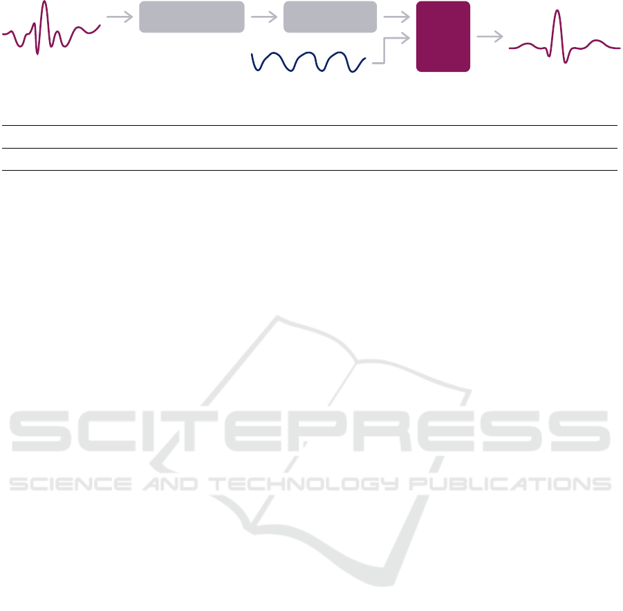
BW FILTERINGNORMALIZATION

Figure 3: Proposed ECG denoising pipeline. Inputs: Noisy ECG and correspondent ACC. Output: Denoised ECG estimate.

Table 1: Useful recorded duration (in minutes) in each session.

A B C D E F G H I J K L M N O P Q R

45.2 27.6 46.1 39.9 31.7 36.1 41.1 31.05 36.1 40.4 41.1 44.4 16.4 17.6 45.4 15.0 47.8 33.1

et al., 2022). One ECG sensor was connected to the

dry conductive plastic electrodes of the chestband,

hence from herein it will be referred to as Band-ECG.

The other ECG sensor was connected to disposable

wet electrodes, hence it will be referred to as Gel-

ECG. Two of the wet electrodes were placed con-

tralateraly on the chest (Lead I), mirroring the textile

electrodes. The ground electrode was placed on the

left iliac crest. Since the activities performed in these

acquisitions involved high-amplitude movement and

high sweat release, the Gel-ECG wet electrodes were

secured in place with Transpore surgical tape, con-

trarily to the wearable dry electrodes. As will be-

come clear ahead, the Gel-ECG signal will be used

as ground-truth of the Band-ECG signal. Hence, both

were placed to capture identical Lead I ECG, as de-

picted in Figure 2.

3.2 Preprocessing

Both ECG sensors included an analogue [0.5, 40] Hz

passband ﬁlter. Two median ﬁlters were applied to

the Band-ECG time series, to estimate BW, the out-

put of which was subtracted from the original ECG,

resulting in BW-free time series. This preprocessing

has been validated in previous works (Xia et al., 2018;

Saraiva, 2022b), for robust real-time BW denoising of

ECG acquired in nonstationary and uncontrolled en-

vironments. Hence, the following experiments on the

Band-ECG start from with this preprocessed time se-

ries, as illustrated in Figure 3.

The Gel-ECG time series were enhanced with a

FIR ﬁlter of [1.2, 40] Hz passing band and order of

250. This is because the Gel-ECG channel will serve

as ground-truth of Lead I ECG of each subject.

No ﬁltering was applied to the ACC time series,

as conveyed in Figure 3.

3.3 Acquisition Protocol

In each session, the volunteers were asked to orderly

perform the following activities:

1. Lift: To repeatedly lift a heavy object;

2. Greetings: To repeatedly handshake and to wave;

3. Gesticulate: To gesticulate while talking;

4. Jumps: To jump repeatedly;

5. Walk-Before: To walk outside before running;

6. Run: To run outside;

7. Walk-After: To walk outside after running.

This protocol was considered to be illustrative of

daily life activities that are prone to hinder ECG qual-

ity. These activities either due to excessive sweat re-

lease, associated motion, or both, usually lead to noise

and artifacts in the recorded biosignals.

For different reasons, not all subjects performed

all activities, and the running and walking durations

were different for each subject. Table 1 shows the use-

ful recorded duration of each session. One of the sub-

jects volunteered for two sessions on different days,

hence there are a total of 18 sessions, identiﬁed from

A to R. In each session, a median of 55 useful minutes

were recorded, summing up to a cohort total of 10.58

hours. By ”useful” it should be understood ”after dis-

carding the periods in which no activity was being ex-

ecuted”.

3.4 Initial Quality Assessment

Cohort median kSQI of Band-ECG channels was 3.5

times lower than that of Gel-ECG signals, convey-

ing that more noise was present on the wearable-

alike ECG. Particularly, Lift, Jumps, Run, and Walk-

After segments showed unacceptable kSQI below 5.

Moreover, the median R peak detection agreement of

two detectors (qSQI) was 1.00 when using Gel-ECG

for all activities, except Jumps (0.98), whereas using

Band-ECG signals was 0.96 on average. In particular,

Run segments showed qSQI below 0.9 for Band-ECG

signals. Therefore, the ECG acquired with the chest

band presents as noisier and with poorer quality than

that acquired with gel electrodes, not necessarily just

because of the differences in hardware, but also due

to its resilience to the executed activities.

Data Augmentation, Multimodality, Subject and Activity Speciﬁcity Improve Wearable Electrocardiogram Denoising with Autoencoders

137

4 DENOISING AUTOENCODER

DAEs were designed to attenuate EMG noise, EDA

noise, MAs, and any other type of process that devi-

ates the Band-ECG waveform from that of the Gel-

ECG. Unlike other denoising methods, DAEs allevi-

ate the need to characterise the noise processes, and

instead they estimate how a version of the signal with-

out noise would look like (Goodfellow et al., 2016).

This is because these models undergo a training pro-

cess with the goal of learning an implicit representa-

tion of the ECG trace without noise. This represen-

tation is an internal state of neural network’s weights

and biases (the model’s parameters) that, when ap-

plied to a noisy ECG segment, output a denoised ver-

sion of it. These parameters are learned from large

datasets of input (noisy) and output (clean) pairs.

4.1 Architecture

As aforementioned in Section 1, it is hypothesised

that the motion information of the torso, present in the

ACC time series, is correlated, causally or not, with

the MAs present in the ECG time series, and that this

information can be used to attenuate them. Hence,

the DAE inputs are (4, 300) matrices, where 4 is the

number of segments (1 ECG + 3 ACC), and 300 is

the number of samples of each, which corresponds to

1 second. The ECG segment is timely synchronised

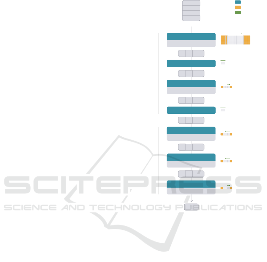
with the ACC segment. Figure 4 illustrates these ma-

trices, as well as the complete network architecture,

which was inspired in (Abecassis et al., 2018). The

network architecture is divided in two modules: en-

coder and decoder.

The encoder task is to represent the input seg-

ments in a latent space, that isolates noise and arti-

facts from the ECG process. In our approach, the en-

coder module has four layers. The input passes ﬁrst

by a 2D convolutional layer that extracts 8 features

with a kernel of size (4, 7). In this process, the kernel

strides (or shifts) every 1 sample. Additionally, three

samples of padding are added to each input. The ac-

tivation function of this layer is the hyperbolic tan-

gent. Then, a maximum pooling layer of kernel size

(2, 1), which strides by two, selects the maximum of

each pair of values in each feature, reducing the fea-

ture length from 300 to 150. A second 2D convo-

lutional layer extracts 4 features using a kernel size

(3, 1), which strides by one. One value of padding is

added to each input feature. The same activation func-

tion is used of this layer. A second maximum pooling

layer, equivalent to the one before, selects the maxi-

mum of each pair of values in each feature, reducing

the feature length from 150 to 75. Therefore, the la-

2D CONVOLUTIONAL

tanh

300

2D T-CONVOLUTIONAL

tanh

2D T-CONVOLUTIONAL

tanh

2D T-CONVOLUTIONAL

tanh

8 1 300

MAX POOLING

8 1 150

2D CONVOLUTIONAL

tanh

4 1 150

MAX POOLING

4 1 75

8 1 150

8 1 300

ECG

300

ECG

ACC X

ACC Y

ACC Z

ENCODER

DECODER

Padding

Layer

Stride

Figure 4: Proposed DAE architecture. Kernel sizes on the

right side of each layer. Tensor sizes in (C, H, W) format.

tent space has a size of 4 features of 75 points each,

i.e., downsampling occurs from 300 to 75 points.

The decoder task is to recover the segment to the

original space, potentially outputting a denoised ver-

sion of the input. The decoder module has three 2D

transpose convolutional layers, that reverse the en-

coder process. The ﬁrst layer takes 4 features and out-

puts 8, using a kernel of size (3, 1). It strides by two

and outputs with (1, 0) padding, increasing the feature

length from 75 to 150. The second layer also outputs

8 features, using a kernel of size (3, 1). It strides by

two and outputs with (1, 0) padding, increasing the

feature length from 150 to 300. These two layers are

activated by the hyperbolic tangent. The last layer en-

compasses the 8 features into 1, using a kernel of size

(3, 1), and has no activation function. Its output is the

potentially denoised ECG segment.

BIOSIGNALS 2023 - 16th International Conference on Bio-inspired Systems and Signal Processing

138

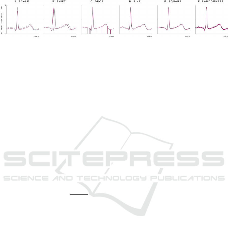
Figure 5: Examples of derived ECG segments when applying data augmentation techniques, in pink. Original time series in

grey. Scale M = 0.85. Shift D = 0.05. Drop p = 0.02. Sine A = 0.02. Square A = 0.01. Randomness A = 0.01. Illustrative

heartbeat segment of 700 ms.

4.2 Training and Evaluation

The DAEs were trained using the Adam optimizer

(Kingma and Ba, 2014). Each network was allowed

to be trained for as many epochs as needed until con-

vergence was reached. Convergence was deﬁned by

the validation loss not decreasing for 20 epochs. The

output loss of each iteration was computed using the

mean squared error (MSE) against the targets, which

were the corresponding Gel-ECG segments. Essen-

tially, given an object (Band-ECG, ACC) the network

should output a segment with minimal error against

the pair target (Gel-ECG). In each experiment, the ex-

amples (object, target) were divided in 20%, trimmed

from the centre of each time series, for the test dataset,

and the remaining 80% of segments would constitute

the train dataset. The train:validation ratio was 8:2.

The denoised estimates,

y, were compared with

their timely corresponding Gel-ECG segment, y, us-

ing the normalized mean squared error (NMSE):

NMSE (dB)

= 10 ·log

||y −

y||

||y −

y||

. (3)

This metric is similar to the MSE, in the sense

that the estimation squared errors are in the numer-

ator, and the normalisation factor in the denominator.

The normalisation factor is the squared errors of the

signal’s mean constant function. Hence, semantically,

the NMSE tells us how good the denoised estimate is

in comparison with the signal’s mean. If the NMSE is

negative, the denoised estimate error is smaller than

the signal’s mean error – which is the desirable. Con-

trarily, if the NMSE is positive, then the signal’s mean

predicts the true signal better than the denoised esti-

mate – which is the undesirable.

Additionally, the ECG SQIs previously described

in Section 2.2 were used to compare the quality of

Band-ECG segments before and after denoising.

5 RESULTS AND DISCUSSION

This section addresses the research questions raised

in Section 1, in the same order they were introduced.

The ECG process can be thought of comprehending

three main sources of variability:

• Environmental: Electrode variability, pressure,

hydration, temperature, and skin conductance in-

troduce variability to the ECG trace. This is ad-

dressed, not only, but primarily, in Subsection 5.1.

• Activity: If the subject is at rest or performing an

activity of some pattern, it introduces variability

to the ECG. This is explored in Subsection 5.2.

• Subject: The subject’s physiology and own way

of wearing the chestband introduce variability to

the ECG trace. This is explored in Subsection 5.3.

5.1 Impact of Data Augmentation

The techniques recently suggested in (Nonaka and

Seita, 2022) were implemented to augment the num-

ber of ECG and ACC segments of each activity. Given

a biosignal segment, similar segments were derived,

without signiﬁcantly altering its original natural mor-

phology, by applying the following operations:

• Scale: Contraction or dillation, in amplitude, by a

multiplier, M (Figure 5A).

• Shift: Left or right translation, in time, by D ×

number of samples (Figure 5B).

• Drop: Multiplication of each sample by zero with

probability p (Figure 5C).

• Sine: Addition of a sinusoidal wave of random

frequency, f , and amplitude A (Figure 5D).

• Square: Addition of a square pulse of random

frequency, f , and amplitude A (Figure 5E).

• Randomness: Addition of gaussian noise of am-

plitude A (Figure 5F).

Parameter M, in Scale, should be between [0.25,1[

for contraction or between ]1, 4] for dilation. Param-

eter D, in Shift, should be between ]0, 1[. The max-

imum displacement is achieved when D = 0.5. The

Data Augmentation, Multimodality, Subject and Activity Speciﬁcity Improve Wearable Electrocardiogram Denoising with Autoencoders

139

Table 2: Average test losses of DAEs trained with datasets augmented ”Multiplier” times, grouped by augmentation technique.

Values in ×10

−3

Multiplier Scale Shift Drop Sine Square Randomness All

10 178.23 111.43 140.82 91.943 81.306 82.924 42.534

50 101.40 93.354 84.532 62.463 41.050 43.263 26.135

100 57.343 49.935 61.930 34.928 22.856 27.050 14.938

shift direction (left or right) is random. Parameter p,

in Drop, should be between ]0, 1[, since it is a proba-

bility. Parameter A should be between ]0, 1] in Sine,

]0, 0.02] in Square and Randomness, so that the nat-

ural biosignal morphology does not get signiﬁcantly

altered. Frequency f is random between [0.001, 0.02]

in Sine, and between [0.001, 0.1] in Square. As il-

lustrated in Figure 5, the derived segments (in pink)

could have very well been acquired in a real scenario,

due to environmental variability.

Universal DAE. On a ﬁrst basis, a DAE to be used

for all subjects and for all activities was trained only

with real examples. There are 37821 examples in the

dataset, which correspond to the total number of sec-

onds reported in Table 1. Herein this and the other

models presented in this subsection will be termed

universal DAEs. The model was trained for 262

epochs, in batches of 64 examples, and initial learn-

ing rate of 0.0005. An average test loss of 0.5305 was

achieved, which is not satisfactory, since the biosig-

nals were normalised in amplitude between 0 and 1.

Different Augmentation Multipliers. The dataset

of real examples was then linearly augmented 10

times with each of the six described techniques, re-

sulting in six augmented datasets, each containing

416031 examples, which corresponds to eleven times

the number of real examples. Six DAEs were trained

and tested with each of these augmented datasets, in

the same conditions as before, and the average test

losses are reported in Table 2. The test loss de-

creased when using each of these augmented datasets.

The same experiment was repeated with datasets aug-

mented 50 times with the same techniques, and test

losses further decreased for every model. Repeating

the experiment with datasets augmented 100 times

also further reduced the test losses of every model,

to one order of magnitude lower than that of the uni-

versal DAE.

Different Augmentation Techniques. Neural net-

works by nature lack explainability, however, in an

attempt to understand these results, one might at-

tribute the success of Sine, Square, and Random-

ness techniques (Table 2) to the fact that they actu-

ally generate different examples in a nonlinear way,

that cannot be traced back to the original examples,

unless the augmentative process that was added is

kept stored, therefore increasing environmental vari-

ability in a nonlinear way. Conversely, Scale, Shift,

and Drop techniques apply linear transformations or

nullify some samples. Scale contracts or expands

the biosignals’ amplitude, which occurs in real envi-

ronments, but most of the waveform characteristics

are still the same. Shift translates segments in time,

which could be achieved by nothing more than seg-

menting the biosignals in a different way. For this

reason, from the next subsection forward only Sine,

Square, and Randomness techniques are employed.

It might seem paradoxical to increase environmental

variability, however the dramatic increase in the num-

ber of examples allows the models to implicitly cap-

ture these environmental differences and to discrimi-

nate them from the ECG pattern, consequently lead-

ing to better generalisations and to avoid underﬁtting.

All Augmentation Techniques. Another experi-

ment was conducted by augmenting the original

dataset all-together with the six techniques, 10, 50 and

100 times. These datasets contained approximately

more than 2.6, 13.2, 26.5 million examples, respec-

tively. The test losses can be found in the last col-

umn of Table 2. It can be concluded that the test

loss decreases by increasing the dataset size. How-

ever, for the dataset augmented 100 times, the test

loss (0.0149) is only 0.0079 lower than the best result

achieved with a dataset generated by a unique tech-

nique (Square, 0.0229), hinting that more examples

do not necessarily lead to signiﬁcant improvements.

Comparisons aside, a test loss of 0.0149 may still not

be satisfactory, as shall be discussed later. In this case,

since segments are normalised in amplitude between

0 and 1, such a loss represents a 1.5% deviation from

the targets, which in artifacts can still appear to be

quite noisy. Activity and subject speciﬁcity strategies

are explored ahead to improve the denoising perfor-

mance. Meanwhile, the impact of data augmentation

will continue to be addressed.

5.2 Impact of Activity Speciﬁcity

The full dataset was divided by activity, including

Baseline when the subjects were at rest in the begin-

ning of the session, into smaller datasets, that is, eight

BIOSIGNALS 2023 - 16th International Conference on Bio-inspired Systems and Signal Processing

140

datasets with the number of examples indicated in Ta-

ble 3. Each of these activity-speciﬁc datasets was also

augmented 50 and 100 times, using Sine, Square, and

Randomness. For each of these, a DAE was trained

for at most 150 epochs, in the same conditions as be-

fore. The test losses are given in Table 4.

Table 3: Total useful duration, in seconds, of each activity.

Lift Greetings Gesticulate Jumps Walk-B Run Walk-A

1262 767 1469 132 2970 26953 2697

When no data augmentation is applied, and only

real examples are used to train the activity-speciﬁc

DAEs, the average test losses are two orders of mag-

nitude lower than that of the best universal DAE.

When the datasets of each activity are augmented,

the average test losses are one order of magnitude

lower than the universal DAEs trained with an aug-

mented dataset. Concretely, the average test loss is

2.5 times smaller for Run DAEs and 12 times smaller

for Baseline DAEs. Gesticulate and Greetings mod-

els achieved the lower test losses. Therefore, activity-

speciﬁc DAEs perform better than non-speciﬁc ones,

at least up to the point of subject variability in task

execution and the environmental differences.

5.3 Impact of Subject Speciﬁcity

Assuming each subject’s dataset is representative

enough to capture the different ways they can exe-

cute an activity, the full dataset was divided by sub-

ject and by activity into smaller datasets, so that only

environmental conditions could inﬂuence the denois-

ing process. Hence, A datasets per subject, being A

the number of activities recorded with each subject.

Each of these datasets was augmented 100 times, us-

ing Sine, Square, and Randomness techniques. For

each of these, a DAE was trained in the same condi-

tions as before. The test losses are reported in the ﬁrst

row of Table 5.

Inspecting the cohort median, when training is

speciﬁc of the subject, the average test loss is one or-

der of magnitude lower for all activities, except for

Jumps and Run, than that of the subject-independent

activity-speciﬁc models. Jumps and Run segments

continue to be the most challenging to denoise, simi-

larly to Table 4. Nonetheless, for Run segments, a me-

dian 0.119% deviation from the target is more accept-

able than that achieved with a subject-independent

DAE. And for some subjects, the Run test loss was

one order of magnitude lower than that of subject-

independent models, such as in session B (0.000429)

and session O (0.000304) (not shown). Moreover,

Baseline’s loss also decreased one order of magni-

tude, and, similar to Table 4, it is the lowest test loss,

which is expected since subjects were at rest in these

periods. Therefore, subject-speciﬁc DAEs perform

better than non-speciﬁc ones, at least up to the point

of environmental differences.

5.4 Importance of Motion Information

One might question if the ACC segments, given along

with the noisy ECG, actually contribute to the de-

noising process, or if the optimiser is minimising the

loss between the noisy and target ECGs by train-

ing the networks to ignore the ACC inputs. The

trained weights immediately after the input layer were

checked and no evidence was found that, up to this

level, the ACC inputs were being nulliﬁed. However,

a much more ﬁne inspection would have to take place

in the remaining trained parameters to answer if and

how this would occur. But we do not need to know

how the networks use the ACC inputs in the denois-

ing process, we simply need to know if they do. To

overcome such a cumbersome study, the same activ-

ity and subject speciﬁc DAEs were retrained with no

ACC information.

In this experiment, per each object, three time

series were still fed to the network along with the

noisy ECG – otherwise the architecture would have

to change – but these time series were fabricated and

were not the real ACC ones. To synthesise ACC,

time series of the same length were generated with

Gaussian noise of zero mean and unit standard devi-

ation, N (0, 1). The same example pairs of objects

and targets were used, however the ACC segments of

each object were replaced by the Gaussian time series,

which has no real motion information. The dataset

was augmented in the same way, and the models were

trained under the same conditions. The median test

losses can be found in the last row of Table 5. The test

MSE in every activity is similar and in the same order

of magnitude as the universal DAE, except for Base-

line segments, meaning these models do not output

satisfactory denoised estimates if the ACC-dedicated

segments are not actually the chest ACC time series.

It is understandable that Baseline models show lower

MSE due to the absence of motion in the input seg-

ments during this period. Therefore, the ACC time

series contain motion information regarding the chest

that is useful to denoise ECG.

5.5 Final Design

The performance of the designed activity and sub-

ject speciﬁc models were validated in a real scenario,

Data Augmentation, Multimodality, Subject and Activity Speciﬁcity Improve Wearable Electrocardiogram Denoising with Autoencoders

141

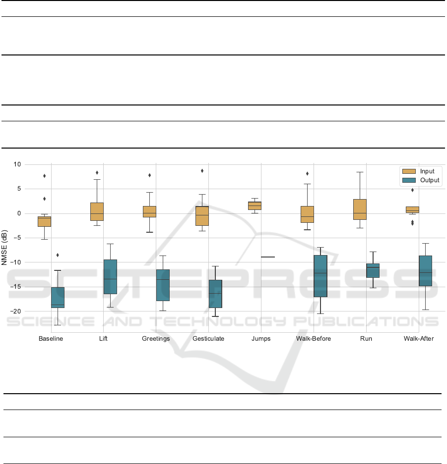
Table 4: Average test losses of DAEs trained with activity-speciﬁc datasets, grouped by augmentation multiplier. Values in

×10

−3

Multiplier Baseline Lift Greetings Gesticulate Jumps Walk-Before Run Walk-After

0 1.660 2.903 4.153 1.723 3.394

3.395 6.381 3.743

50 1.343 2.530 2.034 1.430 3.249 2.991 6.283 2.901

100 1.005 2.000 1.487 1.037 3.027 2.543 5.918 2.396

Trained in batches of 16 examples, because there were not enough examples.

Table 5: Cohort median of average test loss of DAEs trained with activity-speciﬁc and subject-speciﬁc datasets, grouped by

activity. Former row: With real and augmented ACC; Later row: With no real ACC. Values in ×10

−3

Baseline Lift Greetings Gesticulate Jumps Walk-Before Run Walk-After

With ACC 0.172 0.442 0.286 0.211 1.264 0.553 1.198 0.706

No ACC 28.134 908.421 631.102 120.807 937.195 720.910 944.261 852.044

Figure 6: Improvement in NMSE of subject and activity speciﬁc DAEs tested only with real examples.

Table 6: Comparing ECG signal quality indexes (SQIs) before and after denoising steps, grouped by activity. Cohort Quartile

1 (Q1) and Quartile (Q3) values, in the format ”Q1–Q3”. Values in red are below satisfactory the speciﬁc SQI threshold.

Baseline Lift Greetings Gesticulate Jumps Walk-B Run Walk-A

kSQI Input 9.1–14.2 1.4–5.1 3.7–7.5 3.7–12.4 3.4–4.2 1.5–8.1 0.8–2.9 0.9–2.4

kSQI Output 12.4–22.1 10.0–16.5 12.4–20.1 10.1–19.5 11.1-11.3 10.9–15.8 11.3–14.5 9.2–17.3

qSQI Input 0.98–1.00 0.91–0.96 0.95–1.00 0.96–1.00 0.78–0.92 0.94–1.00 0.86–0.99 0.94–1.00

qSQI Output 1.00–1.00 0.94–1.00 0.97–1.00 1.00–1.00 0.97–0.98 0.97–1.00 0.95–1.00 0.98–1.00

where the networks are not tested with augmented

examples. With the same trained parameters, each

DAE was tested with the respective non-augmented

test set, i.e., only with the real examples segmented

from the original time series. For instance, the Run

DAE of session F was tested with a time series of

4.28 minutes, whereas the Lift DAE was tested with

only 29 seconds (cohort durations not shown). The

NMSEs of these inputs and output denoised estimates

against the Gel-ECG are compared in Figure 6. The

denoised median NMSE decreased below −10 dB for

all activities, and Gesticulate NMSE decreased below

−15 dB. Gesticulate, Greetings and Lift segments ob-

tained the higher improvements, respectively, −15.9,

−13.6 and −13.3 dB. Run and Jumps segments ob-

tained the lower improvements, although still valu-

able, of respectively, −11.0 and −10.4 dB. This indi-

cates that the denoised estimations approximate better

the Gel-ECG than the signal’s mean.

The ﬁrst block of Table 6 shows that segments

BIOSIGNALS 2023 - 16th International Conference on Bio-inspired Systems and Signal Processing

142

Figure 7: Example of Walk-Before DAE of session Q. Po-

tentially false R peaks highlighted in yellow.

from all activities, except Baseline, showed unaccept-

able kSQI before denoising (in red). After DAE de-

noising all interquartile kSQI increased. The median

kSQI was higher than 11 for all activities after de-

noising, demonstrating there was less noise present in

the Band-ECG segments after denoising. The second

block of Table 6 shows that the R peaks agreement

by two algorithms was below 0.9 in some Jumps and

Run input segments (in red). After subject and ac-

tivity denoising, the R peaks of these segments were

more salient and unequivocally identiﬁed by the two

different algorithms. Nearly all Baseline and Gestic-

ulate segments showed 1.00 agreement. Therefore,

removal of BW is not sufﬁcient to make better R peak

detections, and the DAE denoising process most con-

tributed to accurate detections. As aforementioned,

particularly in highly noisy environments, it is very

important that R peaks can still be accurately detected

in order to extract HRV features. Figure 7 showcases

an example of how multiple high-amplitude peaks

were attenuated in walking activities. Such high-

amplitude peaks could very well be mistakenly iden-

tiﬁed as R peaks. Moreover, in this example, Q and S

waves were well pronounced in all heartbeats; and P

and T waves were well corrected in most heartbeats,

both in amplitude and in time, to approximate those

of the Gel-ECG (target).

6 CONCLUSIONS

The training process of an ECG-based DAE architec-

ture was studied. The best results for the test dataset

were achieved when DAEs were trained speciﬁcally

for each subject and each activity, with augmented

datasets, and using chest ACC as noise-reference.

Therefore, subject and activity speciﬁcity, data aug-

mentation, and multimodality, together prove as ef-

fecting design techniques to take into consideration

when engineering ECG deep learning models.

It should be noted that it is data augmentation

that possibilities the design of these speciﬁc models,

otherwise there would not be enough subject-speciﬁc

and activity-speciﬁc examples for each subject, gath-

ered from only 55 minutes (median) of multi-activity

sessions. Hence, data augmentation enables subject-

speciﬁc models even from short duration acquisitions.

Moreover, the proposed denoising method has two

main advantages. Firstly, the ECG can be blindly seg-

mented in real-time in 1-second segments, producing

outputs with no ringing effects, therefore dispensing

the need for R peak computation to segment the ECG

by heartbeats. Secondly, the proposed DAE outputs

denoised estimates in polynomial time, since the 2D

convolution operation is majored at O(N

), where N

is the segment number of samples, hence it is feasible

for online denoising in wearables.

ACKNOWLEDGEMENTS

This work was partially funded by the IST re-

search grant BL88/2022, under the scope of project

1018P.06071.1.01.01 ”CardioLeather”, by the

IT research grant BI16/2021, under the project

PCIF/SSO/0163/2019 ”SafeFire”, and by the

Fundac¸

ao para a Ci

encia e Tecnologia (FCT) /

Minist

erio da Ci

encia, Tecnologia e Ensino Supe-

rior (MCTES) research grants 2021.08297.BD and

2022.12369.BD, through national funds and when

applicable co-funded by EU funds.

REFERENCES

Abecassis, L., Ho, M., Tit-Lartey, O., Hwang, W., Gath-

mann, T., Lum, Z., Loong, N. Y., and Moo, J. (2018).

Machine Learning based Denoising of Electrocardio-

gram Signals from a Wearable ECG Monitor. BSc.

Report, Imperial College London, Department of Bio-

engineering.

Abu-Alrub, S., Strik, M., Ramirez, F. D., Moussaoui,

N., Racine, H. P., Marchand, H., Buliard, S.,

ıssaguerre, M., Ploux, S., and Bordachar, P. (2022).

Smartwatch Electrocardiograms for Automated and

Manual Diagnosis of Atrial Fibrillation: A Compar-

ative Analysis of Three Models. Front Cardiovasc

Med, 9:836375.

An, X., Liu, Y., Zhao, Y., Lu, S., Stylios, G. K., and Liu, Q.

(2022). Adaptive Motion Artifact Reduction in Wear-

able ECG Measurements Using Impedance Pneumog-

raphy Signal. Sensors, 22(15):5493.

Arsene, C. (2020). Design of Deep Convolutional Neural

Network Architectures for Denoising Electrocardio-

graphic Signals. In 2020 IEEE Conference on Com-

putational Intelligence in Bioinformatics and Compu-

tational Biology (CIBCB), pages 1–8.

Data Augmentation, Multimodality, Subject and Activity Speciﬁcity Improve Wearable Electrocardiogram Denoising with Autoencoders

143

Ashley, E. A. and Niebauer, J. (2004). Conquering the

ECG. Remedica.

Bansal, A. and Joshi, R. (2018). Portable out-of-hospital

electrocardiography: A review of current technolo-

gies. Journal of Arrhythmia, 34(2):129–138.

Bayoumy, K., Gaber, M., Elshafeey, A., Mhaimeed, O.,

Dineen, E. H., Marvel, F. A., Martin, S. S., Muse,

E. D., Turakhia, M. P., Tarakji, K. G., and Elshazly,

M. B. (2021). Smart wearable devices in cardiovascu-

lar care: Where we are and how to move forward. Nat

Rev Cardiol, 18(8):581–599.

Behbahani, S., Dabanloo, N. J., Nasrabadi, A. M., Teixeira,

C. A., and Dourado, A. (2013). Pre-ictal heart rate

variability assessment of epileptic seizures by means

of linear and non-linear analyses. Anatolian Journal

of Cardiology, 13(8):797–803.

Butt, F. S., La Blunda, L., Wagner, M. F., Sch

afer, J.,

Medina-Bulo, I., and G

omez-Ullate, D. (2021). Fall

Detection from Electrocardiogram (ECG) Signals and

Classiﬁcation by Deep Transfer Learning. Informa-

tion, 12(2):63.

Carmo, A. S., Abreu, M., Fred, A. L. N., and da Silva, H. P.

(2022). EpiBOX: An Automated Platform for Long-

Term Biosignal Collection. Front. Neuroinform., 16.

Chatterjee, S., Thakur, R. S., Yadav, R. N., Gupta, L., and

Raghuvanshi, D. K. (2020). Review of noise removal

techniques in ECG signals. IET Signal Processing,

14(9):569–590.

Chen, L., Yu, H., Huang, Y., and Jin, H. (2021). ECG

Signal-Enabled Automatic Diagnosis Technology of

Heart Failure. J Healthc Eng, 2021:5802722.

Chiang, H.-T., Hsieh, Y.-Y., Fu, S.-W., Hung, K.-H., Tsao,

Y., and Chien, S.-Y. (2019). Noise Reduction in ECG

Signals Using Fully Convolutional Denoising Autoen-

coders. IEEE Access, 7:60806–60813.

Christov, I. I. (2004). Real time electrocardiogram QRS de-

tection using combined adaptive threshold. BioMedi-

cal Engineering OnLine, 3(1):28.

Clifford, G. D., Behar, J., Li, Q., and Rezek, I. (2012).

Signal quality indices and data fusion for determining

clinical acceptability of electrocardiograms. Physiol.

Meas., 33(9):1419–1433.

Goodfellow, I., Bengio, Y., and Courville, A. (2016). Deep

Learning. Adaptive Computation and Machine Learn-

ing. The MIT Press, Cambridge, Massachusetts.

Hamilton, P. (2002). Open source ECG analysis. In Com-

puters in Cardiology, pages 101–104.

Huerta, A., Martinez-Rodrigo, A., Rieta, J., Alcaraz, R.,

and IEEE (2021). ECG Quality Assessment via Deep

Learning and Data Augmentation. In 2021 CINC.

Kavanagh, J. J. and Menz, H. B. (2008). Accelerometry: A

technique for quantifying movement patterns during

walking. Gait & Posture, 28(1):1–15.

Kingma, D. P. and Ba, J. (2014). Adam: A Method for

Stochastic Optimization.

Kutz, M. (2010). Biomedical Engineering and Design

Handbook, Volumes I and II (2nd Edition). McGraw-

Hill Professional Publishing, New York, USA.

Li, Q., Mark, R. G., and Clifford, G. D. (2007). Robust heart

rate estimation from multiple asynchronous noisy

sources using signal quality indices and a Kalman ﬁl-

ter. Physiol. Meas., 29(1):15–32.

Li, Q., Rajagopalan, C., and Clifford, G. D. (2014). A

machine learning approach to multi-level ECG signal

quality classiﬁcation. Comp. Methods Prog. Biomed.,

117(3):435–447.

Mohaddes, F., da Silva, R. L., Akbulut, F. P., Zhou, Y., Tan-

neeru, A., Lobaton, E., Lee, B., and Misra, V. (2020).

A Pipeline for Adaptive Filtering and Transformation

of Noisy Left-Arm ECG to Its Surrogate Chest Signal.

Electronics, 9(5):866.

Mohd Apandi, Z. F., Ikeura, R., Hayakawa, S., and Tsut-

sumi, S. (2020). An Analysis of the Effects of Noisy

Electrocardiogram Signal on Heartbeat Detection Per-

formance. Bioengineering (Basel), 7(2):53.

Munoz-Minjares, J. U., Lopez-Ramirez, M., Vazquez-

Olguin, M., Lastre-Dominguez, C., and Shmaliy, Y. S.

(2021). Outliers detection for accurate HRV-seizure

baseline estimation using modern numerical. Biomed-

ical Signal Processing and Control, 67.

Nonaka, N. and Seita, J. (2022). RandECG: Data Augmen-

tation for Deep Neural Network Based ECG Classi-

ﬁcation. In Takama, Y., Matsumura, N., Yada, K.,

Matsushita, M., Katagami, D., Abe, A., Kashima, H.,

Hiraoka, T., Uchiya, T., and Rzepka, R., editors, Ad-

vances in Art. Intel., volume 1423, pages 178–189.

Nurmaini, S., Darmawahyuni, A., Sakti Mukti, A. N., Rach-

matullah, M. N., Firdaus, F., and Tutuko, B. (2020).

Deep Learning-Based Stacked Denoising and Autoen-

coder for ECG Heartbeat Classiﬁcation. Electronics,

9(1):135.

Pan, Q., Li, X., and Fang, L. (2020). Data Augmentation

for Deep Learning-Based ECG Analysis. In Feature

Engineering and Computational Intelligence in ECG

Monitoring, pages 91–111. Springer, Singapore.

Prieto-Avalos, G., Cruz-Ramos, N. A., Alor-Hern

andez,

G., S

anchez-Cervantes, J. L., Rodr

ıguez-Mazahua, L.,

and Guarneros-Nolasco, L. R. (2022). Wearable De-

vices for Physical Monitoring of Heart: A Review.

Biosensors, 12(5):292.

Raya, M. and Sison, L. (2002). Adaptive noise cancelling of

motion artifact in stress ECG signals using accelerom-

eter. In Proc. of the 2nd Joint 24th Ann. Conf. and

the Ann. Fall Meeting of the Biomedical Eng. Soc.

(IEMBS), volume 2, pages 1756–1757 vol.2.

Reljin, N., Lazaro, J., Hossain, M. B., Noh, Y. S., Cho,

C. H., and Chon, K. H. (2020). Using the Re-

dundant Convolutional Encoder–Decoder to Denoise

QRS Complexes in ECG Signals Recorded with an

Armband Wearable Device. Sensors, 20(16):4611.

Rodrigues, J., Belo, D., and Gamboa, H. (2017). Noise

detection on ECG based on agglomerative clustering

of morphological features. Computers in Biology and

Medicine, 87:322–334.

Saraiva, J. (nov-2022a). Deep Residual Learning for

Epileptic Seizure Prediction and Tools to Expedite

Biosignal Research. MSc. Thesis, Department of

Computer Science and Engineering, Instituto Superior

ecnico, Universidade de Lisboa, Lisbon.

BIOSIGNALS 2023 - 16th International Conference on Bio-inspired Systems and Signal Processing

144

Saraiva, J. (nov-2022b). Denoising and Artifact Re-

moval of Ambulatory Electrocardiogram for Patient

Continuous-Monitoring. MSc. Thesis, Department of

Bioengineering, Instituto Superior T

ecnico, Universi-

dade de Lisboa, Lisbon.

Semmlow, J. L. and Griffel, B. (2014). Biosignal and Med-

ical Image Processing. CRC Press, 3rd ed. edition.

Vandecasteele, K., Cooman, T. D., Chatzichristos, C.,

Cleeren, E., Swinnen, L., Ortiz, J. M., Huffel, S. V.,

umpelmann, M., Schulze-Bonhage, A., Vos, M. D.,

Paesschen, W. V., and Hunyadi, B. (2021). The power

of ECG in multimodal patient-speciﬁc seizure moni-

toring: Added value to an EEG-based detector using

limited channels. Epilepsia, 62(10).

Xia, Y., Zhang, H., Xu, L., Gao, Z., Zhang, H., Liu, H.,

and Li, S. (2018). An Automatic Cardiac Arrhyth-

mia Classiﬁcation System With Wearable Electrocar-

diogram. IEEE Access, 6:16529–16538.

Xiong, P., Wang, H., Liu, M., and Liu, X. (2015). De-

noising Autoencoder for Eletrocardiogram Signal En-

hancement. Journal of Medical Imaging and Health

Informatics, 5(8):1804–1810.

Data Augmentation, Multimodality, Subject and Activity Speciﬁcity Improve Wearable Electrocardiogram Denoising with Autoencoders

145