FInC Flow: Fast and Invertible k × k Convolutions for Normalizing Flows
Aditya Kallappa, Sandeep Nagar and Girish Varma
International Institute of Information Technology, Hyderabad, India
Keywords:
Normalizing Flows, Deep Learning, Invertible Convolutions.
Abstract:
Invertible convolutions have been an essential element for building expressive normalizing flow-based gen-
erative models since their introduction in Glow. Several attempts have been made to design invertible k × k
convolutions that are efficient in training and sampling passes. Though these attempts have improved the ex-
pressivity and sampling efficiency, they severely lagged behind Glow which used only 1 × 1 convolutions in
terms of sampling time. Also, many of the approaches mask a large number of parameters of the underlying
convolution, resulting in lower expressivity on a fixed run-time budget. We propose a k × k convolutional
layer and Deep Normalizing Flow architecture which i.) has a fast parallel inversion algorithm with running
time O(nk
2
) (n is height and width of the input image and k is kernel size), ii.) masks the minimal amount of
learnable parameters in a layer. iii.) gives better forward pass and sampling times comparable to other k × k
convolution-based models on real-world benchmarks. We provide an implementation of the proposed parallel
algorithm for sampling using our invertible convolutions on GPUs. Benchmarks on CIFAR-10, ImageNet, and
CelebA datasets show comparable performance to previous works regarding bits per dimension while signifi-
cantly improving the sampling time.
1 INTRODUCTION
Normalizing flow is an important subclass of Deep
Generative Models that offers distinctive benefits
(Kobyzev et al., 2020). In comparison to GANs
(Goodfellow et al., 2014a) and VAEs (Kingma et al.,
2019), they are trained using a very intuitive Maxi-
mum Likelihood loss function. Images and the latent
vector, which is required to have a Gaussian distri-
bution, correspond one-to-one in flow models. De-
spite these intriguing characteristics, GANs and VAEs
are utilized more frequently. This is due to the need
for the Normalizing Flows transformations to be in-
vertible, which significantly restricts the neural net-
work types employed. For deployment in a real-world
scenario, the invertible transformations must be effi-
ciently calculable in the forward and sample stages.
A significant breakthrough came with Glow
(Kingma and Dhariwal, 2018) which used 1 × 1 in-
vertible convolutions to design normalizing flows. If
it exists, the inverse function for a 1 × 1 convolution
also happens to be a 1 × 1 convolution. Since com-
puting 1 × 1 convolution has fast parallel algorithms
for which running time does not depend on the spatial
dimensions, they are also highly efficient in forward
pass (i.e. computing latent vector from an image) as
well as the sampling passes (i.e. computing image
from a sampled latent vector). Extending Glow to use
invertible k × k convolutions promises to improve the
expressivity further, allowing it to model more com-
plex datasets. However, this is a challenging prob-
lem since the inverse function for a k × k convolu-
tion, in general, is given by a n
2
× n
2
matrix where
n = H = W (i.e. the spatial dimensions). Hence, while
the forward pass can be fast, the trivial approach for
the sampling pass will cost O(n
4
) operations per con-
volutional layer.
CInC Flow (Nagar et al., 2021) introduced a
padded 3 × 3 convolution layer design and gave it
the necessary and sufficient conditions to make it in-
vertible. They showed that the convolution matrix
is lower triangular by ensuring padding in only two
sides of the input. Furthermore, all the diagonal en-
tries of the convolution matrix are equal to a single
weight parameter. By setting this parameter to 1, they
ensured that the convolutions are invertible, and Jaco-
bian is always 1.
We build on their work by proposing a parallel in-
version algorithm for their convolution design. The
parallel algorithm only uses O(nk
2
) sequential opera-
tions, unlike O(n
2
k
2
) operations used by most previ-
ous works. We also build a normalizing flow archi-
338
Kallappa, A., Nagar, S. and Varma, G.
FInC Flow: Fast and Invertible k k Convolutions for Normalizing Flows.
DOI: 10.5220/0011876600003417
In Proceedings of the 18th International Joint Conference on Computer Vision, Imaging and Computer Graphics Theory and Applications (VISIGRAPP 2023) - Volume 5: VISAPP, pages
338-348
ISBN: 978-989-758-634-7; ISSN: 2184-4321
Copyright
c
 2023 by SCITEPRESS – Science and Technology Publications, Lda. Under CC license (CC BY-NC-ND 4.0)

Figure 1: Convolution of a 3 × 3 TL (Top Left) padded image with a 2 × 2 filter viewed as a linear transform of vectorized
input(x) by the convolution matrix M. The TL padding on the input results in the making matrix M lower triangular, and all
diagonal values correspond to w
k,k
of the filter. Each row of M can be used to find a pixel value. The rows or pixels with the
same color can be inverted in parallel since all the other values required for computing them will already be available at a step
of our inversion algorithm 1.
tecture, where channel-wise splitting is further used
to parallelize operations.
Our Contributions.
1. We design a k × k invertible convolutional layer
with a fast and parallel invertible sampling algo-
rithm (see Sections 4.1, 4.2).
2. We build a normalizing flow architecture based on
the fast invertible convolution, which uses channel
wise splitting to improve the parallelism further
(see Sections 4.3, 4.4).
3. We provide a fast GPU implementation of our par-
allel inversion algorithm and benchmark the sam-
pling times of the model (see Section 5). We show
greatly improved sampling times due to our paral-
lel inversion algorithm, while giving similar bits
per dimensions as compared to other works.
2 RELATED WORK
Generative Modeling. The idea of generative mod-
eling stems from training a generative model whose
sample comes from the same distribution as the train-
ing data distribution. Most of the generative models
can be grouped as Generative adversarial networks
(GANs) (Goodfellow et al., 2014b; Brock et al.,
2019), Energy-based models (EBMs) (Zhang et al.,
2022; Song et al., 2021a), Variational autoencoders
(VAEs) (Kingma and Welling, 2013; Kingma et al.,
2019; Hazami et al., 2022), Autoregressive models
(Oord et al., 2016; Nash et al., 2020), Diffusion mod-
els (Ho et al., 2020; Song et al., 2021b; Song and
Ermon, 2019) and Flow-based models (Dinh et al.,
2014, 2017; Hoogeboom et al., 2019; Kingma and
Dhariwal, 2018; Ho et al., 2019; Ma et al., 2019; Na-
gar et al., 2021).
Normalizing Flows. Flows-based models construct
complex distributions by transforming a probabil-
ity density through a series of invertible mappings
(Rezende and Mohamed, 2015). At the end of these
invertible mapping, we obtain a valid distribution;
hence, this type of flow is referred to as a Normalizing
Flow model. Flow models apply the rule for change
of variables; the initial density ‘flows’ through the
sequence of invertible mappings (Dinh et al., 2017).
Flow-based models generalize a dataset distribution
into a latent space (Kobyzev et al., 2020).
Invertible kxk Convolutions. An invertible neural
network requires the inverse of the network with fast
and efficient computation of the Jacobian determinant
(Song et al., 2019). An invertible neural network can
be used for generation and classification with more
interpretability. (Kingma and Dhariwal, 2018) pro-
posed an invertible 1 × 1 convolution building on top
of NICE (Dinh et al., 2014) and RealNVP (Dinh et al.,
2017) consisting a series of flow step combined in a
multi-scale architecture. Each flow step consists of
actnorm followed by an invertible 1 × 1 convolution,
followed by a coupling layer (see Sec 4.3). Emerging
(Hoogeboom et al., 2019) presented method to gen-
eralized 1 × 1 convolution to invertible k × k convo-
lutions. Emerging chains two specific auto regressive
convolutions (Kingma and Welling, 2013) to form a
single convolutional layer following the associativity
of the convolution operation. Each of these autore-
gressive convolutions is chosen such that the result-
ing convolution matrix M is triangular with an inverse
time of each of the convolutions is O(n × n × k
2
).
MintNet (Song et al., 2019) presented a method for
designing invertible neural networks by combining
building blocks with a set of composition rules. The
inversion of the proposed blocks necessitates a se-
quence of dependent computations that increase the
FInC Flow: Fast and Invertible k k Convolutions for Normalizing Flows
339

Table 1: Comparison of the learnable parameters. where n × n is input size, k × k is filter size which is constant, c is number
of input/output channels. d is the number of latent dimensions. # of ops: required number of operations for the inversion of
convolutional layers. The complexity of Jacobian: Time complexity for calculating the Jacobian of a single convolution layer.
For FInC Flow and CInC Flow, the Jacobian is 1, since the Convolution matrix is lower triangular with diagonal entries being
1.
Method # of ops # params / CNN layer Complexity of Jacobian Inverse
FInC Flow (our) (2n −1)k
2
k
2
− 1 1 exact
Woodbury (Lu and Huang, 2020) cn
2
k
2
O(d
2
(c +n)+ d
3
) exact
MaCow (Ma et al., 2019) 4nk
2
k(⌈
k
2
⌉ − 1) O(n
3
) exact
Emerging (Hoogeboom et al., 2019) 2n
2
k
2
k(⌈
k
2
⌉ − 1) O(n) exact
CInC Flow (Nagar et al., 2021) n
2
k
2
k
2
− 1 1 exact
MintNet (Song et al., 2019) 3n
k
2
3
O(n) approx
SNF (Keller et al., 2021) k
2
k
2
approx approx
network’s sampling time. SNF (Keller et al., 2021)
proposed a method to reduce the computation com-
plexity of the Jacobian determinant by replacing the
gradient term with a learned approximate inverse for
each layer. This method avoids the determinant of
Jacobian and makes it approximate, and requires an
additional backward pass for inversion of convolu-
tion. MaCow (Ma et al., 2019) while many other pa-
pers make use of the invertibility of triangular matrix
to reduce inversion time, MaCow outperforms all of
them by performing the inverse in O(nk
2
) by care-
fully masking 4 kernels at the top, left, bottom, right
to achieve a full convolution, but this flow model use
four autoregressive convolutions to make an effec-
tive standard convolution. Woodbury (Lu and Huang,
2020) this paper employs the Woodbury transforma-
tion for invertible convolution, which is a generalized
permutation layer that models dimension dependen-
cies along the channel and spatial axes using the chan-
nel and spatial transformation. ButterflyFlow (Meng
et al., 2022) introduced a new family of an invertible
layer that works for special underlying structures and
needs a sequence of layers for an effective invertible
convolution.
Fast Algorithms for Invertible Convolutions.
CInC Flow (Nagar et al., 2021), derive necessary and
sufficient conditions on a padded CNN for it to be
invertible and require a single CNN layer for every
effective invertible CNN layer. The padded CNN can
leverage the advantage of parallel computation for in-
version, resulting in faster and more efficient compu-
tation of Jacobian determinants.
The distinguishing feature of our invertible con-
volutions as compared to previous works is that we
have a parallel inversion algorithm that does only
(2n − 1)k
2
operations where n is input size and k is
kernel size. MaCow is the closest approach that takes
twice the number of operations. Some of the ap-
proaches, like MintNet and SNF, do achieve a lesser
number of operations. However, they are not proper
normalizing flows as they compute only an approx-
imate inverse. We use the convolution design from
CInC Flow but give a parallel inversion algorithm
for it. Furthermore, our FInC Flow Unit is designed
to efficiently parallelize the operations by splitting
the convolution operations channel-wise. In Table 1,
we compare our proposed flow model with the ex-
isting model in terms of the receptive fields/number
of learnable parameters, complexity of computing the
inverse of convolution layer for sampling.
3 PRELIMINARIES
Normalizing Flows. Formally, Normalizing Flows
is a series of transformations of a known simple prob-
ability density into a much more complex probability
density using invertible and differentiable functions.
These invertible function allows to write the proba-
bility of the output as a differentiable function of the
model parameters. As a result, the models can be
trained using backpropagation with the negative log
likelihood loss function.
Let X ∈ R
d
be a random variable with tractable
density p
X
. Let f : R
d
→ R
d
be a differentiable and
invertible function. If Y = f (X) then the density of Y
can be calculated as
p
X
(x) = p
Y
(y)


detJ
f


where J
f
=
∂ f (x )
∂x
.
Note that J
f
is a d × d matrix called the Jacobian.
If X is transformed using a sequence of functions f
i
’s.
That is f = f
1
◦ f
2
◦ f
3
◦ ··· ◦ f
r
. Now probability den-
sity, p
Y
(y) can be expressed as
p
Y
(y) = p
X
( f
−1
(y)) ·
1
∏
i=r
|J
f
−1
i
(y
i
)|. (1)
VISAPP 2023 - 18th International Conference on Computer Vision Theory and Applications
340

where y
i
= f
−1
i
◦ · ·· ◦ f
−1
r
(x). The log-probability of
p
Y
which will be used to model the complex image
distribution is given by,
log p
Y
(y) = log p
X
( f
−1
(y
r
)) +
r
∑
i=1
log|det J
f
−1
i
(y
i
)|.
(2)
The functions f
−1
i
will be given by neural network
layers and the above function can be computed dur-
ing the forward pass of the neural network. The nega-
tive of this function called the negative log likelihood
(NLL) is minimized when images in the dataset are
given highest probabilities. Hence it gives a simple,
interpretable loss function for training the model.
Invertible Convolutions. The convolution of an in-
put X with shape H × W × C with a kernel K with
shape k × k ×C ×C is Y = X × K of shape (H − (k +
1)) × (W − (k + 1)) ×C which is equal to
Y
i, j,c
o
=
∑
l,h<k
C
∑
c
i
=1
X
i+l, j+k,c
i
K
l,k,c
i
,c
o
(3)
Notice that the dimensions of X and Y are not neces-
sarily the same. To ensure that the X and Y are the
same size, we apply padding to the input X. For an
input image X with shape H × W × C, the (t, b, l, r)
padding of X is the image
ˆ
X of shape (H + t + b) ×
(W + l + r) ×C is defined as
ˆ
X
i, j,c
=
(
X
i−t, j−l,c
if i −t < H and j − l < W
0 otherwise
(4)
The convolution operation is a linear transformation
of the input. For the vectored (flattened) input X, de-
noted by x, the output vector y can be written as y =
Mx. Matrix M is the called as the Convolution Matrix
and the dimensions of this matrix is HWC × HWC.
As long as matrix M is invertible, the convolutional
layer can be included as a part of the Normalizing
Flows. The common approach to building invertible
convolutions is by making M upper triangular and en-
suring invertibility by making diagonal entries to be
nonzero.
Algorithms for Computing Inverse of Convolu-
tions. For normalizing flows built using invertible
convolutions, the sampling pass will involve comput-
ing the inverse of the convolution matrix. This in-
volves solving a linear systems of equations Mx = y.
For a general square matrix of size n × n, the time
complexity for inversion is O(n
3
). For a lower tri-
angular matrix of size n × n, the time complexity
for inversion is O(n
2
) because of back-substitution
method. Notice that the size of convolution matrix,
M) is n
2
× n
2
(refer Figure 1) and also that row of
the matrix has only k
2
entries at the maximum, re-
sults in an inversion time of O(n
2
k
2
) which is used in
many of the previous works like Emerging and CInC
Flows. We show that this method can be parallelized
for carefully designed convolutions giving a complex-
ity of only O(nk
2
).
4 FInC FLOW: OUR APPROACH
In this section we describe our approach including
convolution layer design which has a fast parallel in-
version algorithm with running time O(nk
2
). For
more clarity, we refer to height of the image as H,
width as W and channels as C in this section.
4.1 Convolution Design
As it is obvious from equation x = M
−1
y, the in-
verse timings depends on M. Emerging (Behrmann
et al., 2019) masks almost half of the convolution ker-
nel values to ensure M is a Lower Triangular Matrix.
However, we follow the method followed in CInC
Flow, where only a few values of the convolution ker-
nel are masked. For an input image X with shape
H ×W ×C, the top-left(TL) i.e., (t, 0, l, 0) padding of
X is the image X
(TL)
of shape (H + t) × (W + l) ×C
is defined in equation 5 and similarly for the top-right
(TR) as equation 6, bottom-left (BL) as equation 7,
bottom-right (BR) as equation 8.
X
(TL)
i, j,c
=
(
X
i−t, j−l,c
i −t > 0 ∧ j − l > 0
0 otherwise
(5)
X
(TR)
i, j,c
=
(
X
i−t, j,c
i −t > 0 ∧ j − r < W
0 otherwise
(6)
X
(BL)
i, j,c
=
(
X
i, j−l,c
i − b < H ∧ j − l > 0
0 otherwise
(7)
X
(BR)
i, j,c
=
(
X
i, j,c
i − b < H ∧ j − r < W
0 otherwise
(8)
Figure 1 shows the convolution of a TL padded 3 × 3
image with a 2×2 filter is equivalent to a matrix mul-
tiplication between convolution matrix M and vec-
tored input x . We leverage this to find the inverse
faster. We discuss this in more detail in the subse-
quent sections. Also padded input X
(TR)
, X
(BL)
and
X
(BR)
are equivalent to X
(TL)
once they are flipped
along corresponding dimension(s).
FInC Flow: Fast and Invertible k k Convolutions for Normalizing Flows
341

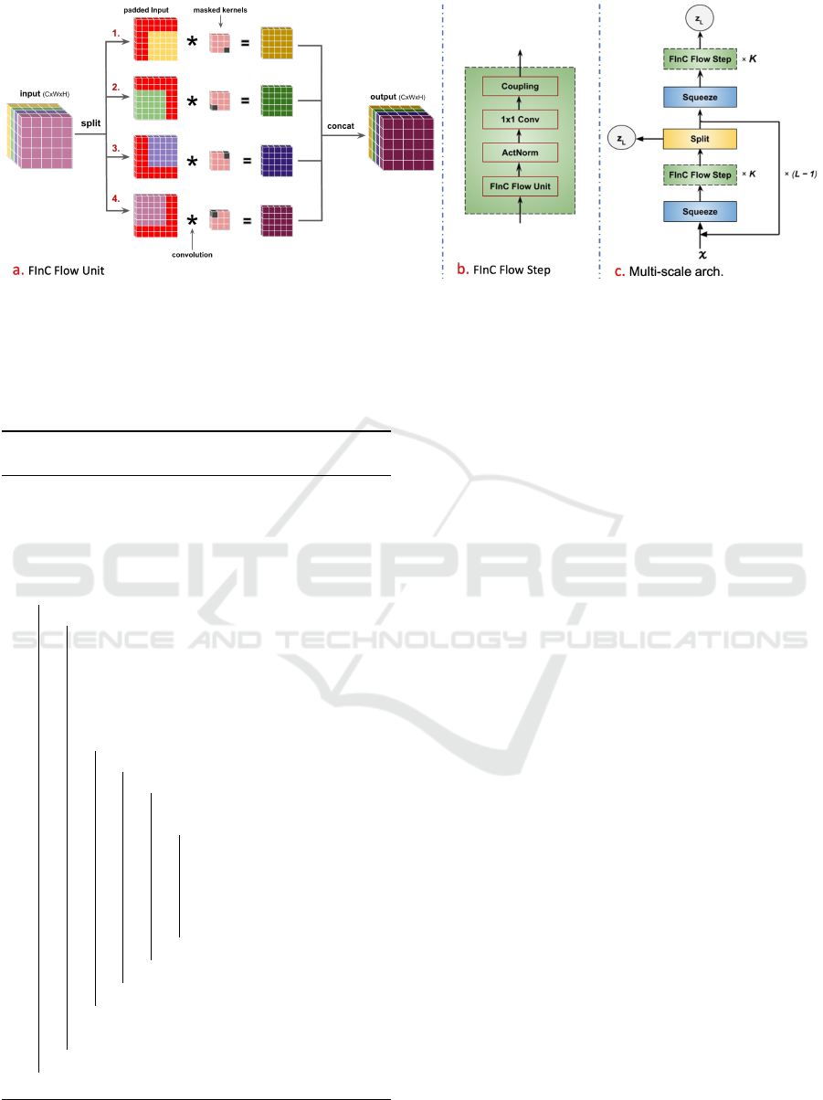
Figure 2: (a) FInC Flow unit: to utilize the independence of convolution on channels the input channels are sliced into four
equal parts and then padded (1. top-left, 2. top-right, 3. bottom-right, 4. bottom-left) to keep the input size and output
size same. Next, parallelly convoluted each sliced channel with the corresponding masked kernel (masked corner of kernels:
1. bottom-right, 2. bottom-left, 3. top-left, 4. top-right). Finally, concatenate the output from each convolution. (b) We
propose a FInC Flow architecture 4.3 where each FInC Flow Step consists of an actnorm step, followed by an invertible 1 × 1
convolution, followed by coupling layer. (c) Flow is combined with a multi-scale architecture 4.4.
Algorithm 1: Fast Parallel Inversion Algorithm of
TL padded convolution block(PCB).
Input: K: Kernel of shape (C,C, k
H
, k
W
)
Y : output of the conv of shape (C, H,W )
Result: X: inverse of the conv. with shape
(C, H,W ).
1 Initialization: X ← Y ;
2 for d ← 0, H +W − 1 do
3 for c ← 0,C − 1 do
/* The below lines of code
executes parallelly on
different threads on GPU
for every index (c, h, w) of
X on the dth diagonal. */
4 for k
h
← 0, k
H
− 1 do
5 for k
w
← 0, k
W
− 1 do
6 for k
c
← 0,C − 1 do
7 if pixel (k
c
, h − k
h
, w − k
w
)
not out of bounds then
8 X[c, h, w] ←
X[c, h, w] − X[k
c
, h −
k
h
, w − k
w
] ∗
K[c,k
c
, k
H
− k
h
−
1, k
W
− k
w
− 1];
9 end
10 end
11 end
12 end
/* synchronize all threads */
13 end
14 end
4.2 Parallel Inversion Algorithm
We have presented our algorithm in Algorithm 1. The
algorithm can be understood using Figure 1.
Definition 1 (Diagonal Elements). Two pixels x
i, j
and x
i
′
, j
′
are said to be secondary diagonal elements
if i + i
′
= j + j
′
. For brevity, we refer to these ele-
ments from here on simply as Diagonal Elements.
Theorem 1 proves that every element of on the
diagonal can be computed parallelly and Line 2 of
the algorithm takes care of that. We initialize X to
Y in Line 1 and compute X in Line 8 which is given
in Equation 10. It is important that we wait for the
threads to synchronize before we move to the next di-
agonal, as they are needed for computing the elements
of the next diagonal. The not out of bounds in Line 7
means we are remaining in the k ×k convolution win-
dow and also we are not including pixel (i, j) while
computing x
i, j
as given in Equation 10
Theorem 1. The inverse of the pixels on the diag-
onals of a TL padded convolution can be computed
independently and parallelly.
Proof. The (i, j)
th
pixel value of the output Y with
shape H ×W can be calculated as
y
i, j
= (M
iW + j,:
)
T
· x
which means y
i, j
is the dot product of M
iW + j,:
i.e.,
the corresponding row of matrix M and the vectored
input x. Because it is a TL padded convolution, y
i, j
depends only on the values of k × k window of x
≤i,≤ j
pixels where x
≤i,≤ j
are the pixels that are on the top
and left side of the pixel x
i, j
including x
i, j
. Because
VISAPP 2023 - 18th International Conference on Computer Vision Theory and Applications
342

all the diagonal values are w
k,k
, we have,
y
i, j
= w
k,k
x
i, j
+ f (x
<i,< j
)
x
i, j
=
y
i, j
− f (x
<i,< j
)
w
k,k
where x
<i,< j
are the pixels which are strictly top
and left side of (i, j). Following the masking pattern
of CInC Flow, we have w
k,k
= 1 and f is a linear func-
tion which is given by weighted sum of the given pix-
els weighed by the filter values. So,
x
i, j
= y
i, j
− f (x
<i,< j
) (9)
x
i, j
= y
i, j
−
k
∑
p=0
k
∑
q=0
x
i−p, j−q
K
p,q
where p = q ̸= 0
(10)
Let two pixels x
i, j
and x
i
′
, j
′
be on the same diag-
onal. This also means that only one of the follow-
ing settings is true a) i < i
′
and j > j
′
or b) i > i
′
or
j < j
′
. Either way, we can conclude that computa-
tion of x
i, j
is not dependent on x
i
′
, j
′
and vice versa
following the result in Equation 9. Hence they can be
computed independently. Once x
i, j
is computed, fol-
lowing the Equation 9 and the above result, we can
compute x
i+1, j
and x
i, j+1
. Since, the sets of pixels
x
<i+1,< j
and x
<i,< j+1
both include the elements of
x
<i, j
and also x
i, j
, we can write
x
i+1, j
= y
i+1, j
− f (x
<i+1,< j
)
= y
i+1, j
− αx
i, j
− f
1
(x
<i,< j
) (11)
x
i, j+1
= y
i, j+1
− f (x
<i,< j+1
)
= y
i, j+1
− βx
i, j
− f
2
(x
<i,< j
) (12)
where α and β are kernel weights.
From Equations 11 and 12, we can conclude that
x
i+1, j
and x
i, j+1
which are on the same diagonal can
be calculated parallelly in a single step.
Theorem 2. Algorithm 1 uses only (H + W − 1)k
2
sequential operations.
Proof. We have proved in Theorem 1 that the inverse
pixels on a single diagonal can be computed parallelly
in one iteration of Algorithm 1. Since there are H +
W − 1 number of diagonals in a matrix and there are
at maximum k
2
entries in a row of the convolutional
matrix, the number of sequential operations needed
will be (H +W − 1)k
2
.
Thus the running time of our algorithm is O(nk
2
)
where n = H = W
4.3 FInC Flow Unit
Figure 2a visualizes our k × k convolution block. We
call this block as FInC Flow Unit. We use all the
4 padding techniques mentioned before to different
channels of the image. For this purpose, we split the
input into four equal parts along the channel axis. We
do TL padding to the first part, TR to the second part,
BL to the third part and TR to the fourth part. Then we
use a masked filter on each of these parts to perform
the convolution operation parallelly. We call each of
this padded image along with it’s corresponding ker-
nel as Padded Convolution Block (PCB).
4.4 Architecture
Figure 2c shows the complete architecture of our
model. Our model architecture resembles the archi-
tecture of Glow. The multi-scale architecture involves
a block of a Squeeze layer, FInC Flow Step repeated
K number of times and a Split layer. The whole block
is repeated L − 1 number of times. A Squeeze layer
follows this and finally FInC Flow Step repeated K
times. At the end of each split layer, half of the chan-
nels are ’split’ (taken away) and modeled as Gaussian
distribution samples. These splited half channels are
latent vectors. The same is done for the output chan-
nels. These are denoted as z
L
in Figure 2(c). Each
FInC Flow Step consists of a FInC Flow Unit, an Act-
norm Layer, a 1×1 Convolutional Layer, followed by
a coupling layer.
Actnorm Layer: Acts as an activation normalization
layer similar to that of a batch normalization layer. In-
troduced in Glow, this layer performs the affine trans-
formation using scale and bias parameters per chan-
nel.
1 × 1 Convolutional Layer: This layer introduced in
Glow does a 1 × 1 convolution for a given input. Its
log determinant and inverse are very easy to compute.
It also improves the effectiveness of coupling layers.
Coupling Layer: RealNVP introduced a layer in
which the input is split into two half. The first half re-
mains unchanged, and the second half is transformed
and parameterized by the first half. The output is
concatenation of first half and the affine transforma-
tion, by functions parameterized by the first, of sec-
ond half. The inverse and log determinant of coupling
layer are computed in a straightforward manner. Cou-
pling layer consists of 3×3 convolution followed by a
1×1 and a modified 3×3 convolution used in Emerg-
ing.
Squeeze: This layer takes features from spatial to
channel dimension (Behrmann et al., 2019), i.e., it re-
duces the feature dimension by total four, two across
FInC Flow: Fast and Invertible k k Convolutions for Normalizing Flows
343

Table 2: Comparison of the bits per dimension (BPD), forward pass time (FT) and sampling time (ST) on standard benchmark
datasets of various k × k convolution based Normalizing Flow models. FT and ST are presented in seconds.
Model MNIST CIFAR-10 Imagenet-32x32 Imagenet-64x64
BPD FT ST BPD FT ST BPD FT ST BPD FT ST
Emerging – 0.16 0.62 3.34 0.49 17.19 4.09 0.73 25.79 3.81 1.71 137.04
MaCow – – – 3.16 1.49 3.23 – – – 3.69 2.91 8.05
CInC Flow – – – 3.35 0.42 7.91 4.03 0.62 11.97 3.85 1.57 55.71
MintNet 0.98 0.16 17.29 3.32 2.09 230.17 4.06 2.08 230.44 – – –
FInC Flow (our) 1.05 0.14 0.09 3.39 0.37 0.41 4.13 0.48 0.52 3.88 1.43 2.11
the height dimension and two across the width dimen-
sion resulting in increases the channel dimension by
four. As used by (Dinh et al., 2017), we use squeeze
layer to reshape the feature maps to have smaller res-
olution but more channels.
Split: Input is splited into two halves across the chan-
nel dimension. We retain the first half, and a function
parameterized by first half transform the second half.
The transformed second half is modeled as Gaussian
samples, are the latent vectors. We do not use the
checkerboard pattern used in RealNVP (Dinh et al.,
2017) and many others to keep the architecture sim-
ple.
5 RESULTS
Bits Per Dimension (BPD): BPD is closely related
to NLLLoss given in equation 2. BPD of H ×W ×C
image is given by
bpd =
NLLLoss × log
2
e
HWC
(13)
Table 2 shows the BPD comparative results of vari-
ous models with our model. We present the results
of MaCow-var which uses Variational Dequantization
which was introduced in Flow++ (Ho et al., 2019).
BPDs recorded are the reported numbers from the re-
spective model papers.
Sampling Time: Table 2 shows the comparative re-
sults of our model with other models. For MaCow,
we use the official code released by the authors. We
use the code for Emerging, which was implemented
in PyTorch by the authors of SNF.. We have imple-
mented CInC Flow in PyTorch and used it to generate
results. The FTs and STs are recorded by averaging
ten runs on untrained models (including our model).
In Figure 3, we plot the relationship between the
input image size and inverse sampling time. As the
input image size increase, our Parallel Inversion Al-
gorithm improve by utilizing the independence in the
convolution matrix M. If we input a single image
(batch size = 1), our model performs similarly to the
CInC Flow and Emerging. MaCow is far slower be-
cause it does the masking of four kernels to maintain
the receptive field. To do one convolution, it needs
four convolutions to complete one standard convolu-
tion, making it slower. Emerging requires two consec-
utive autoregressive convolutions to have the same re-
ceptive field as standard convolution and solver com-
pared to FInC Flow. For batch size = 4 and larger,
FInC Flow beats the Emerging, MaCow , and CInC
Flow by a big difference (see Figure 3) while main-
taining the same receptive field.
Scaling Sampling Time with Spatial Dimensions:
Table 3 shows the comparison among the invertible
convolution-based models. To keep it fair, we restrict
the total parameters across all the models to be close
to 5 M. We note down the average sampling time (ST)
to generate 100 images over ten runs while doubling
the size of the sampled image from 16×16 all the way
to 128 × 128 and also doubling our batch size from 1
all the way to 128. Our model outperforms all the
other models in most, if not all, the settings. All the
models were untrained and run on a single NVIDIA
GTX 1080Ti GPU.
Image Reconstruction and Generation: In Fig-
ure 4, we present the effectiveness of the FInC Flow
model in the reconstruction (sampling) of the images.
First, we feed the input image to forward flow and get
the latent vector (z
L
). To reconstruct the images from
the latent vector (z
L
), give the z as input to the in-
verse flow. Figure 4 present the reconstructed face im-
ages for the CelebA dataset after training our model
for 100 epochs. The model takes a random sample
from the Gaussian distribution for the latent vector to
generate sample images. This latent vector is used
to generate images by going backward in the flow
model. In Figure 5, we present generated sample by
our model on the MNIST, CIFAR-10, and ImageNet-
64x64 dataset.
VISAPP 2023 - 18th International Conference on Computer Vision Theory and Applications
344

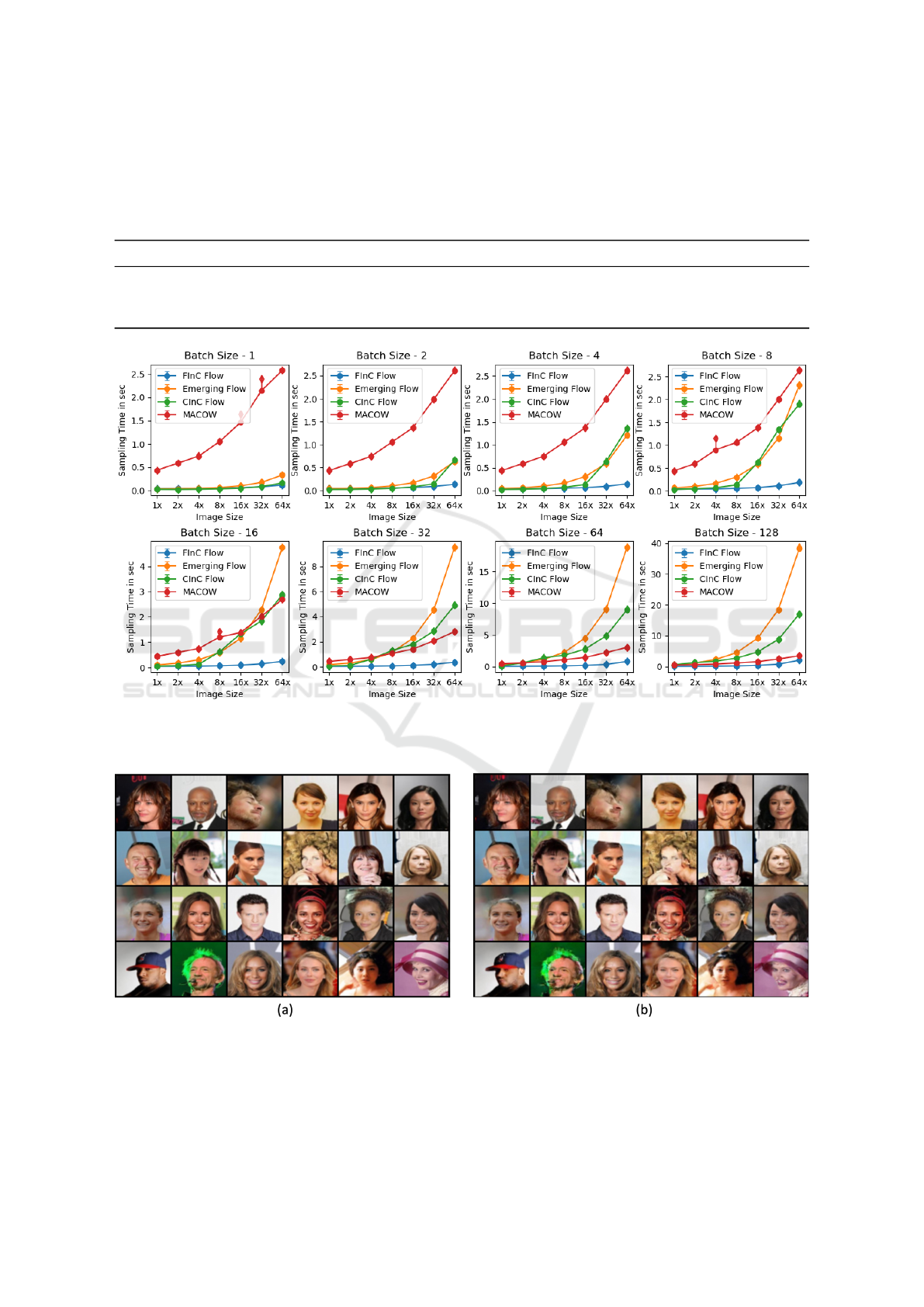
Table 3: CIFAR-10: comparison of learnable parameters and the sampling time. FInC Flow has less number of learnable
parameters with the same receptive field and fast layers (all the times are averaged over ten loops for n = 100 sample images
in seconds). ST = Sample time, FT = Forward Time. MaCow-FG is the fine-grained MaCow model and MaCow-org stands
for MaCow model utilizes the original multi-scale architecture which is the same as Glow. MaCow and our method is closely
similar in term of the convolutional design. So, here we show that our proposed method do fast sampling while maintaining
the faster forward time.
Models Setting (K and L) Learnable params (M = million) FT(n=100) ST(n=100)
MaCow-FG [4, [12, 12], [12, 12], 12] 37.19M 0.88 2.64
MaCow-org [4, [12, 12], [12, 12], 12], [4, 4] 38.4M 1.48 3.23
FInC Flow (our) [28, 28, 28] 39.46M 0.37 0.41
Figure 3: Sampling Times for four models - our, Emerging, CInC Flow, MaCow. Each plot gives the 95% Confidence Interval
(CI) time of the ten runs to sample 100 images. X-axis represents the sizes of the image sampled starting from 16 × 16 × 2
(H ×W ×C) all the way to 128 × 128 × 2.
Figure 4: Comparison of (a) original and (b) reconstructed image samples for the 64 × 64 CelebA dataset after FInC Flow
model for 100 epochs. From the images, we can conclude our model reconstruct original image.
FInC Flow: Fast and Invertible k k Convolutions for Normalizing Flows
345

Figure 5: Uncurated generated samples images from our
flow model.
6 CONCLUSION
With a parallel inversion approach, we present a k × k
invertible convolution for Normalizing flow models.
We utilize it to develop a model with highly efficient
sampling pass, normalizing flow architecture. We
implement our parallel algorithm on GPU and pre-
sented benchmarking results, which show a signif-
icant enhancement in forward and sampling speeds
when compared to alternative methods for k × k in-
vertible convolution.
REFERENCES
Behrmann, J., Grathwohl, W., Chen, R. T., Duvenaud,
D., and Jacobsen, J.-H. (2019). Invertible residual
networks. In International Conference on Machine
Learning, pages 573–582. PMLR.
Brock, A., Donahue, J., and Simonyan, K. (2019). Large
scale GAN training for high fidelity natural image
synthesis. In International Conference on Learning
Representations.
Deng, L. (2012). The mnist database of handwritten digit
images for machine learning research. IEEE Signal
Processing Magazine, 29(6):141–142.
Dinh, L., Krueger, D., and Bengio, Y. (2014). Nice: Non-
linear independent components estimation. arXiv
preprint arXiv:1410.8516.
Dinh, L., Sohl-Dickstein, J., and Bengio, S. (2017). Density
estimation using real nvp. In International Conference
on Learned Representations.
Goodfellow, I., Pouget-Abadie, J., Mirza, M., Xu, B.,
Warde-Farley, D., Ozair, S., Courville, A., and Ben-
gio, Y. (2014a). Generative adversarial nets. In
Ghahramani, Z., Welling, M., Cortes, C., Lawrence,
N., and Weinberger, K., editors, Advances in Neural
Information Processing Systems, volume 27. Curran
Associates, Inc.
Goodfellow, I., Pouget-Abadie, J., Mirza, M., Xu, B.,
Warde-Farley, D., Ozair, S., Courville, A., and Ben-
gio, Y. (2014b). Generative adversarial nets. Advances
in neural information processing systems, 27.
Hazami, L., Mama, R., and Thurairatnam, R. (2022).
Efficient-vdvae: Less is more. arXiv preprint
arXiv:2203.13751.
Ho, J., Chen, X., Srinivas, A., Duan, Y., and Abbeel, P.
(2019). Flow++: Improving flow-based generative
models with variational dequantization and architec-
ture design. In International Conference on Machine
Learning, pages 2722–2730. PMLR.
Ho, J., Jain, A., and Abbeel, P. (2020). Denoising diffusion
probabilistic models. Advances in Neural Information
Processing Systems, 33:6840–6851.
Hoogeboom, E., Van Den Berg, R., and Welling, M.
(2019). Emerging convolutions for generative normal-
izing flows. In International Conference on Machine
Learning, pages 2771–2780. PMLR.
Keller, T. A., Peters, J. W., Jaini, P., Hoogeboom, E., Forr
´
e,
P., and Welling, M. (2021). Self normalizing flows.
In International Conference on Machine Learning,
pages 5378–5387. PMLR.
Kingma, D. P. and Ba, J. (2015). Adam: A method for
stochastic optimization. In Bengio, Y. and LeCun,
Y., editors, 3rd International Conference on Learn-
ing Representations, ICLR 2015, San Diego, CA, USA,
May 7-9, 2015, Conference Track Proceedings.
Kingma, D. P. and Dhariwal, P. (2018). Glow: Generative
flow with invertible 1x1 convolutions. Advances in
neural information processing systems, 31.
Kingma, D. P. and Welling, M. (2013). Auto-encoding vari-
ational bayes. arXiv preprint arXiv:1312.6114.
Kingma, D. P., Welling, M., et al. (2019). An introduction
to variational autoencoders. Foundations and Trends®
in Machine Learning, 12(4):307–392.
Kobyzev, I., Prince, S. J., and Brubaker, M. A. (2020). Nor-
malizing flows: An introduction and review of current
methods. IEEE transactions on pattern analysis and
machine intelligence, 43(11):3964–3979.
Krizhevsky, A. (2009). Learning multiple layers of features
from tiny images.
Liu, Z., Luo, P., Wang, X., and Tang, X. (2015). Deep
learning face attributes in the wild. In Proceedings
of the IEEE international conference on computer vi-
sion, pages 3730–3738.
Lu, Y. and Huang, B. (2020). Woodbury transformations
for deep generative flows. Advances in Neural Infor-
mation Processing Systems, 33:5801–5811.
Ma, X., Kong, X., Zhang, S., and Hovy, E. (2019). Macow:
Masked convolutional generative flow. Advances in
Neural Information Processing Systems, 32.
Meng, C., Zhou, L., Choi, K., Dao, T., and Ermon, S.
(2022). Butterflyflow: Building invertible layers with
butterfly matrices. In International Conference on
Machine Learning, pages 15360–15375. PMLR.
Nagar, S., Dufraisse, M., and Varma, G. (2021). CInc flow:
Characterizable invertible 3$\times$3 convolution. In
The 4th Workshop on Tractable Probabilistic Model-
ing.
Nash, C., Ganin, Y., Eslami, S. A., and Battaglia, P. (2020).
Polygen: An autoregressive generative model of 3d
meshes. In International conference on machine
learning, pages 7220–7229. PMLR.
Oord, A. v. d., Dieleman, S., Zen, H., Simonyan, K.,
Vinyals, O., Graves, A., Kalchbrenner, N., Senior,
A., and Kavukcuoglu, K. (2016). Wavenet: A
VISAPP 2023 - 18th International Conference on Computer Vision Theory and Applications
346

generative model for raw audio. arXiv preprint
arXiv:1609.03499.
Rezende, D. and Mohamed, S. (2015). Variational inference
with normalizing flows. In International conference
on machine learning, pages 1530–1538. PMLR.
Russakovsky, O., Deng, J., Su, H., Krause, J., Satheesh, S.,
Ma, S., Huang, Z., Karpathy, A., Khosla, A., Bern-
stein, M., et al. (2015). Imagenet large scale visual
recognition challenge. International journal of com-
puter vision, 115(3):211–252.
Song, Y., Durkan, C., Murray, I., and Ermon, S. (2021a).
Maximum likelihood training of score-based diffusion
models. Advances in Neural Information Processing
Systems, 34:1415–1428.
Song, Y. and Ermon, S. (2019). Generative modeling by
estimating gradients of the data distribution. Advances
in Neural Information Processing Systems, 32.
Song, Y., Meng, C., and Ermon, S. (2019). Mintnet: Build-
ing invertible neural networks with masked convolu-
tions. Advances in Neural Information Processing
Systems, 32.
Song, Y., Sohl-Dickstein, J., Kingma, D. P., Kumar, A.,
Ermon, S., and Poole, B. (2021b). Score-based gen-
erative modeling through stochastic differential equa-
tions. In International Conference on Learning Rep-
resentations.
Zhang, D., Malkin, N., Liu, Z., Volokhova, A., Courville,
A., and Bengio, Y. (2022). Generative flow networks
for discrete probabilistic modeling. In Chaudhuri, K.,
Jegelka, S., Song, L., Szepesvari, C., Niu, G., and
Sabato, S., editors, Proceedings of the 39th Interna-
tional Conference on Machine Learning, volume 162
of Proceedings of Machine Learning Research, pages
26412–26428. PMLR.
ADDITIONAL DETAILS
Code to our implementation is available here: https:
//github.com/aditya-v-kallappa/FInCFlow
Datasets. We train our model on standard bench-
mark datasets MNIST (Deng, 2012), CIFAR-10
(Krizhevsky, 2009), and ImageNet (Russakovsky
et al., 2015) sampled down to 32×32 and 64×64. We
also train our model on CelebA (Liu et al., 2015) sam-
pled down to 64 × 64. Figure 4a present the CelebA-
64 × 64 reconstructed samples and Figure 5b for the
CIFAR-10 and ImageNet-64x64 generated samples.
Hyperparameters. To train our model, we use
Adam optimizer (Kingma and Ba, 2015) with learn-
ing rate of 0.001 with an exponential decay of
0.99997 per epoch. For training on Imagenet, we also
make sure that the gradients stay between −1 and +1
by clipping them.
Masking To make sure the masked values in the
Padded Conv Blocks, we ensure they are not affected
by back propagation. To achieve this, we reset the
gradients of the masked values to zero after every
training iteration.
Cuda Code Details. To run CUDA code, we use
PyTorch-LTS 1.8.2 and cudatoolkit 10.2. While we
can implement Algorithm 2 to find inverse of each
padded block individually, we can take advantage of
the fact that all 4 Padded Conv Blocks are equiva-
lent after proper flipping of padded inputs and kernels.
This is done by using Algorithm 2 on GPU.
First we split Y into 4 parts across channel dimension
following the architecture shown in 2. This is given
in Line 1. Then we flip Y and kernels to match TL-
padding which is given in Line 2. Then we concate-
nate them to get the final Y and K respectively which
are given in Lines 3 and 4. Then we apply Algorithm
2 to find the inverse. We do the reverse process of
the above to get the correct X. The steps are given in
Lines 5, 6, 7, 8.
We fix the number of threads of each grid of the GPU
to be 1024, the number of grids
x
to be the batch size
and grids
y
to be 4 which is the number of Padded
Conv Blocks in a single FInC Flow Unit. This en-
sures that not only GPU inverts the whole FInC Flow
Unit at once but also on a batch of images.
Algorithm 2: Fast Parallel Inversion Algorithm for
FInC Flow Unit.
Input: K
1
, K
2
, K
3
, K
4
- Convolution Kernels
of different PCB, Y - Output of the
FInC Flow Unit
Result: X - Input to the FInC Flow Unit /
Inverse of the FInC Flow Unit
1. Y
1
,Y
2
,Y
3
,Y
4
← split(Y )
2. Flip Y
2
,Y
3
,Y
4
, K
2
, K
3
, K
4
(inplace) appropriately
to match TL padding
3. X ← concat(Y
1
,Y
2
,Y
3
,Y
4
)
4. K ← concat(K
1
, K
2
, K
3
, K
4
)
5. Apply Algorithm 1 with input K,Y to get X
6. X
1
, X
2
, X
3
, X
4
← split(X)
7. Flip X
2
, X
3
, X
4
appropriately to get the correct
output
8. X ← concat(X
1
, X
2
, X
3
, X
4
)
Running MaCow, Emerging, CInC Flow, SNF.
For MaCow and SNF, we use the official code re-
FInC Flow: Fast and Invertible k k Convolutions for Normalizing Flows
347

leased by the authors. Emerging was implemented in
PyTorch by the authors of SNF. We make use of that.
We have implemented CInC Flow on PyTorch to get
the results.
Computing Run-time and Confidence Intervals.
We run the model (both forward and sampling) 11
times and ignore the 1
st
run as it includes the initial-
ization time. We calculate the mean, standard devi-
ation and 95% confidence interval and plot the num-
bers.
To calculate forward time, we pass 100 images, as for
sampling times, we sample 100 images. We present
these numbers in Table-3.
For sampling time comparison of different models
shown in Figure 3, we set the total number of param-
eters for all the models to be close to 5M to make it a
fair comparison.
Hardware/Training Time. Our hardware setup
consists of Intel Xeon E5-2640 v4 processor pro-
viding 40 cores, 80 GB of DDR4 RAM, 4 Nvidia
GeForce GTX 1080 Ti GPUs each with 12 GB of
VRAM. We train our model on all GPUs using Py-
Torch’s Data Parallel class. We implement early stop-
ping mechanism for smaller datasets like MNIST,
CIFAR-10. For others we train the model for a max-
imum epochs. To evaluate Forward Time and Sam-
pling Time, we use only one of the GPUs.We eval-
uate our FInC Flow model on MNIST, CIFAR-10,
Imagenet-32x32, and Imagenet-64x64 datasets for
three metrics - (a) Loss expressed in Bits per Dimen-
sion (BPD), (b) Forward Pass Time (FT): Time taken
for 100 images to be passed through the model and (c)
Sampling Time(ST): Time taken by the model to gen-
erate 100 images. To do this, we train our model with
Adam Optimizer with a learning rate (lr ) of 0.001
and exponentially reduce the lr by 0.99997 after each
epoch. We have used 4 NVIDIA GTX 1080 Ti GPUs
to train our model. Evaluation(FT/ST) is done on a
single GPU.
VISAPP 2023 - 18th International Conference on Computer Vision Theory and Applications
348