Latent Code Disentanglement Using Orthogonal Latent Codes and

Inter-Domain Signal Transformation

Babak Solhjoo

and Emanuele Rodol

Department of Computer Science, Sapienza University of Rome, Via Salaria 113, Rome, Italy

Keywords:

Variational Auto Encoders, Artiﬁcial Intelligence, Orthogonal Latent Code, Disentanglement, Hybrid,

Inter-Domain Signal Transfer, Image, Voice.

Abstract:

Auto Encoders are speciﬁc types of Deep Neural Networks that extract latent codes in a lower dimensional

space for the inputs that are expressed in the higher dimensions. These latent codes are extracted by forcing

the network to generate similar outputs to the inputs while limiting the data that can ﬂow through the network

in the latent space by choosing a lower dimensional space (Bank et al., 2020). Variational Auto Encoders

realize a similar objective by generating a distribution of the latent codes instead of deterministic latent codes

(Cosmo et al., 2020). This work focuses on generating semi-orthogonal variational latent codes for the inputs

from different source types such as voice, image, and text for the same objects. The novelty of this work

is on aiming to obtain uniﬁed variational latent codes for different manifestations of the same objects in the

physical world using orthogonal latent codes. In order to achieve this objective, a speciﬁc Loss Function has

been introduced to generate semi-orthogonal and variational latent codes for different objects. Then these

orthogonal codes have also been exploited to map different manifestations of the same objects to each other.

This work also uses these codes to convert the manifestations from one domain to another one.

1 INTRODUCTION

The VAEs are able to generate latent codes for the

data where these latent codes can be later used to gen-

erate new samples or used for other purposes such as

noise removal. However, in the original version of the

VAEs, there is no way to place the latent codes in the

desired places in the latent space. These codes are

generated through the training process automatically

and the trainer has almost no control over their loca-

tion. This can be problematic in certain cases when

there is an interest in obtaining a certain code in the

latent domain. Moreover, the generated code for the

same objects with different manifestations will be dif-

ferent. For instance, if there is an image of an ”Ap-

ple”, and the recorded voice of the word ”Apple”, the

generated latent code will be different for them since

the data domain is different. However, having a com-

mon code for the same features would be useful. This

is very similar to the human brain which is able to

comprehend a feature or an object such as an apple de-

spite the fact that the incoming data might have differ-

ent data domains. Most of the research on the VAE is

https://orcid.org/0000-0003-3771-1255

https://orcid.org/0000-0003-0091-7241

concentrated over a single domain of the data. There

is limited research on a network with the capability of

handling data coming from different domains of the

data.

This work aims to propose a method using which

it is possible to generate similar codes for the same

features coming from different data domains. The

method uses orthogonal codes in the latent domain

for each unique feature. Then these codes are used

to transfer the data from one domain to another one.

More speciﬁcally this work shows the possibility of

transferring voice signals to the image domain. The

applications of such a system are countless ranging

from search engines to creating an AI technology with

the capability of processing information from multi-

ple channels and combining them. In addition, having

unique codes provide the possibility to develop spe-

cialized networks independently over separate data

domains and integrate them later.

2 RELATED WORKS

Artiﬁcial Neural Networks (ANN) are a set of net-

works inspired by biological neural networks. These

Solhjoo, B. and Rodolà, E.

Latent Code Disentanglement Using Orthogonal Latent Codes and Inter-Domain Signal Transformation.

DOI: 10.5220/0011860200003393

In Proceedings of the 15th International Conference on Agents and Artiﬁcial Intelligence (ICAART 2023) - Volume 2, pages 427-436

ISBN: 978-989-758-623-1; ISSN: 2184-433X

 2023 by SCITEPRESS – Science and Technology Publications, Lda. Under CC license (CC BY-NC-ND 4.0)

427

networks are constructed from a set of neurons that

simply sum up the inputs from other neurons or in-

puts with a speciﬁc weight and then apply an activa-

tion function over the results. Each neuron might be

interconnected with many other neurons. Assuming

the use of non-linear activation functions in these net-

works, these complex networks can be used to solve

and address complex problems(Hopﬁeld, 1985)(Guo

et al., 2022).

In (Hopﬁeld, 1985), the authors use ANN net-

works to show the possibility of using these net-

works for optimizing different problems. The authors

speciﬁcally apply these networks to Traveling Sales-

man Problem which is known as a complex optimiza-

tion problem and represent its power over solving this

problem.

In the literature different ANN architectures are

proposed to address different sets of problems. Dis-

crete Hopﬁeld Neural Networks (DHNN), is a spe-

ciﬁc type of ANN network that is designed to address

the combinatorial problem. These networks divided

the neurons into the input and output neurons and neu-

rons are either in bipolar (-1,1) or binary (0,1) states.

The lack of a symbolic rule to represent the connectiv-

ity of the neurons is one of the problems in the DHNN

networks. In (Guo et al., 2022), authors propose a

novel logical rule that is capable of mixing system-

atic logical rules with non-systematic logical rules by

exploiting a random clause generator.

The Variational Auto Encoders are another type

of ANN network that can be used in different ﬁelds

such as compressing, de-noising, and generating data.

These networks are constructed from two main parts

known as Encoder and Decoder. Encoders and De-

coders are constructed using multi-layers of neural

networks. The network has a bottleneck in the middle

with a low capacity to pass the information from the

Encoder network to the Decoder side of the network

forcing the system to generate a lower dimensional

representation of each signal known as latent codes.

In (Cosmo et al., 2020) VAE is used to generate de-

formable 3D shapes with higher accuracy. This sys-

tem uses a disentanglement technique by dividing the

latent space into two sub-spaces, one part dedicated

to intrinsic features of the 3D shapes and the other to

extrinsic features of the shape. By this method, each

sub-space of the latent code stores a speciﬁc type of

data related to the object. This algorithm uses three

Loss Functions for training which are Reconstruc-

tion, Interpolation, and Disentanglement. The Dis-

entanglement Loss term itself is also obtained from a

combination of two terms that are disentanglement-

int, and disentanglement-ext.

In (Pu et al., 2016), a speciﬁc conﬁguration of

VAE is used to predict the labels and captions for the

images. In this system, a Convolutional Neural Net-

work (CNN) is used as an encoder and a Deep Gen-

erative Deconvolutional Network (DGDN) as a de-

coder. The mentioned latent codes are also fed into a

Bayesian Support Vector Machine (BSVM) to gener-

ate labels. It is also connected to a Recurrent Neural

Network (RNN) to generate captions for the images

using their latent code. In this work, the latent space is

shared between the DGDN network which is respon-

sible for decoding and reconstruction of the images,

and the BSVM or RNN network. The training of the

network has been done by minimizing the variational

lower bound of the Cost Function.

In (Venkataramani et al., 2019), a VAE is used for

source separation. To realize this objective this sys-

tem learns a shared latent code space between mixed

and clear voice signals. This work considers source

separation as a style transfer problem in VAEs. It as-

sumes the mixture data is actually a clean voice mixed

up with some noises and hence the objective of the

network is to transfer the style of input and represent

it as the output which is a clean form of the signal.

In (Sadeghi and Alameda-Pineda, 2020) and

(Sadeghi et al., 2020), VAEs have been used to en-

hance voice quality using audio-visual information.

This model exploits the visual data of lips movements

in addition to the audio data. The main idea is that

although the voice might be recorded improperly or

degraded by the noise, the visual data of lip move-

ments are mostly untouched and extractable. In this

work, the Short Time Fourier Transform (STFT) of

the voice is extracted in the ﬁrst step which provides

the frequency representation of the voice signals in

each time frame. The VAE is trained using these bins

and learns the latent domain distribution for the voice

signals. The lower bound of the Likelihood Function

ELBO is maximized to estimate the parameters of the

network. In addition to this Audio VAE (AVAE) net-

work, this method introduces two networks to fetch

the speech data from the visual inputs which are re-

ferred to as Base Visual VAE (BVVAE) and Aug-

mented Visual VAE (AVVAE). The inputs of these

networks are actually lips images that are captured

and centered using computer vision methods. The

BVVAE is a two-layered fully connected network.

Finally, in order to obtain a combined audio-visual

model, the Conditional VAE (CVAE) framework has

been exploited. For training the combined model, the

network is provided with the data as well as the re-

lated class labels in order to estimate the data distri-

bution.

In (Palash et al., 2019), the authors use a VAE

in processing the textual data in order to transfer the

ICAART 2023 - 15th International Conference on Agents and Artiﬁcial Intelligence

428

style of the text. More speciﬁcally, a VAE is used to

convert positive texts to negative ones and vice versa.

To do so, an encoder network is implemented fol-

lowed by two different decoders. One of the decoders

is responsible for generating positive styles and the

other is responsible to generate negative styles. The

sentences are given associated with some tags. These

tags are converted to numerical values ranging from

-2 to 2 which represent ”Surely Negative”, ”Slightly

Negative”, ”Neutral”, ”Slightly Positive” and ”Surely

Positive” and evaluation is done by the resultant nu-

merical values.

In (Wang et al., 2018), the authors reviewed the

use of the KL Divergence Function. In the normal

VAEs, KL divergence is used to compare the similar-

ity of two distributions. However, there are two main

problems with KL divergence measure. First, the KL

divergence does not satisfy the trigonometric distance

Equation. It means that there is no clear relation be-

tween D

(P||Q) + D

(Q||L) and D

(P||L). The

other problem is related to the fact that the divergence

increases as the overlap between two distributions de-

creases which means that if two distributions do not

have any overlap the divergence will increase to in-

ﬁnity and consequently the gradient will be lost. To

solve these problems, in this method, Hellinger dis-

tance is exploited along with CVAE to produce music.

The Hellinger distance is non-negative, symmetric,

and trigonometric. The generated music results with

Helinger distance provide a better subjective feeling

and also need lower latent space dimensions to gen-

erate the same music in comparison to the original

model.

In (Wang et al., 2019), a Gated Recurrent Unit

(GRU) is exploited to build a Variational Recurrent

Auto-Encoders (VRAE) to model music generation in

the symbolic domain. In this system, there are three

GRU encoders that are responsible to encode the note

features dT

, T

, and P

. Another GRU in the encoder

is responsible to capture the context vector from the

other three encoders. The note unrolling is realized

by a decoder network which is composed of 7 GRUs.

Three of these GRUs are responsible for modeling

attribute-speciﬁc context. One is modeling the con-

textual unit and three are for constructing the note el-

ements. The hierarchical decoder proceeds with note

generation in three steps. First, it produces the dT

based on note

t−1

. Then using this information and

again using note

t−1

the T

is extracted. In the ﬁnal

step using all previous information, the pitch is gen-

erated.

As mentioned although these works apply the

VAEs to different domains of the data, they are con-

centrated only on one speciﬁc domain. Also, there

Table 1: Hardware used for training and testing the Voice

VAE.

Minimum hardware requirements for Voice VAE

Device Speciﬁcations

CPU Intel(R) Core(TM) i7-8750H @2.20

2.21 GHz

GPU NVIDIA GeForce RTX 2070 with

Max-Q Design

Disk 512GB SSD + 1TB HDD

RAM 32.0 GB

Type 64bit

is almost no control over the placement of the la-

tent codes in the latent domain. In the next section,

we propose a method for constructing a model using

which a speciﬁc code can be generated in the latent

domain for the object signals coming from the differ-

ent signal domains.

3 PROPOSED MODEL

In this work, we propose a system that is able to gen-

erate similar orthogonal codes for the same features

of the objects coming from different data domains.

The method described in this section is tested over the

voice, image, and text domains, however, the method

can be generalized to any other domains. The details

of the hardware used to train and test the models are

listed in Table 1.

3.1 Voice Model

The ﬁrst model is designed to generate unique orthog-

onal codes for the voice signals. The dataset used for

this purpose is the MNIST-Voice dataset. The model

is constructed using a 10-layer encoder and 10-layer

decoder network. The encoder and decoder networks

are chosen to be symmetric. Figure 1 represents the

model structure.

The ﬁrst and last layers of the encoder and decoder

networks are normalization layers. In this layer, a new

normalization method is implemented and we call it

Max M% normalization. This method sorts the sig-

nals from the maximum value to the minimum. Then

the M value with the maximum amplitude is selected

and their average is calculated. The signal is nor-

malized using this value. This normalization method

gives better results in comparison to simple max nor-

malization or STD normalization.

Table 2 lists the details of the layers in this net-

work. The Activation Functions of each layer is se-

lected to be Relu in order to add non-linearity to the

model while avoiding the problems caused vanishing

Latent Code Disentanglement Using Orthogonal Latent Codes and Inter-Domain Signal Transformation

429

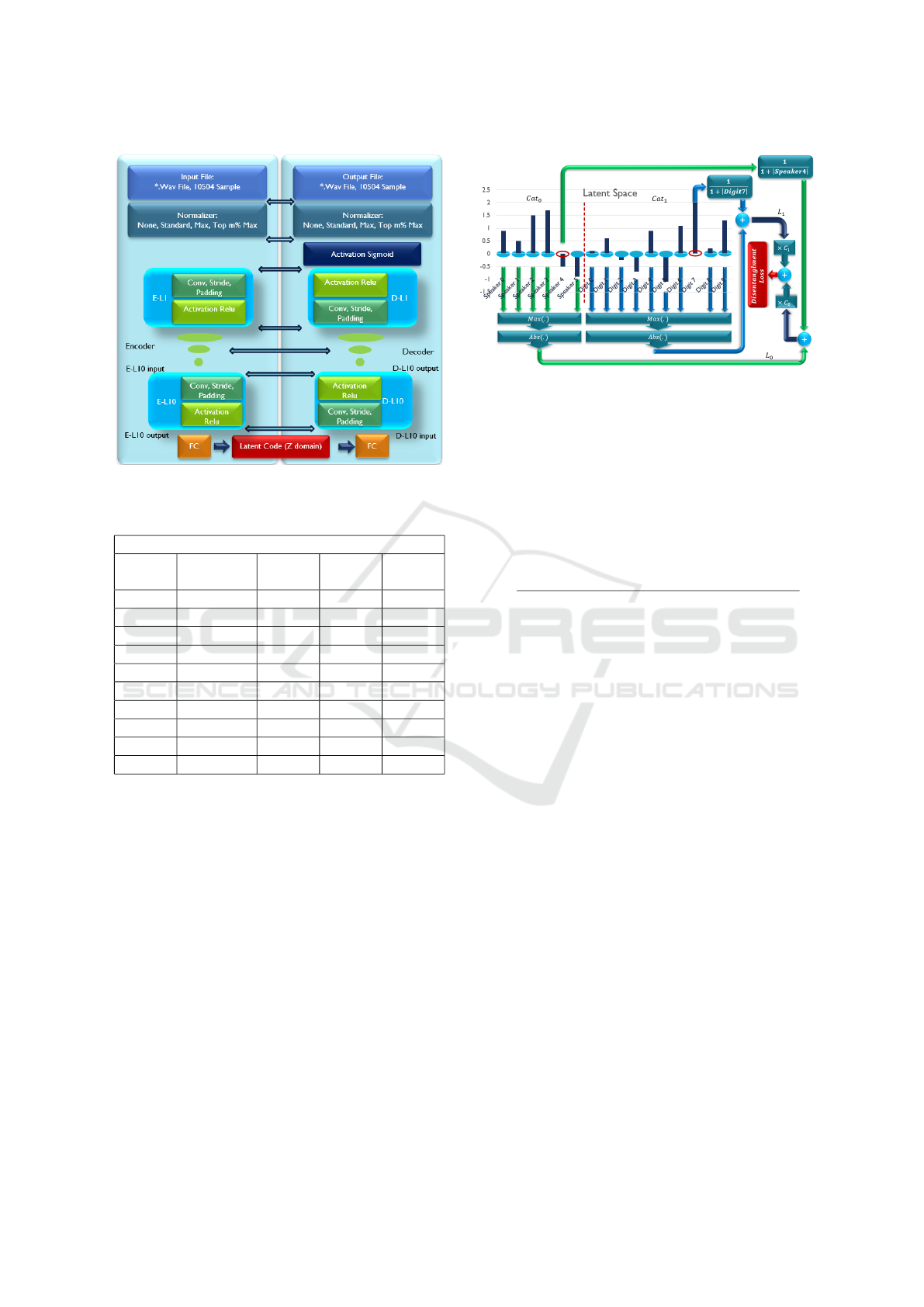
Figure 1: Proposed Voice VAE architecture.

Table 2: Convolutional layer details for Voice VAE.

Details of each convolutional layer for Voice-VAE

Layer

Index

Output

Channels

Kernels

Size

Stride Padding

L1 1026 64 16 1

L2 285 32 8 1

L3 79 16 2 1

L4 76 8 1 1

L5 73 7 1 1

L6 70 6 1 1

L7 67 5 1 1

L8 64 4 1 1

L9 62 4 1 1

L10 60 3 1 1

gradient. Only in the last layer, in the decoder side

there is also a Sigmoid Activation Function in order to

smooth the generated signal, suppress the spike values

and normalize it between 0 and 1.

After the convolutional layers, there is a fully

connected layer and its output is ﬂattened. The la-

tent domain is logically divided into categories. The

codes obtained from the fully connected layer are nor-

malized using the related category vector amplitude.

Then the sampling is done using a Gaussian distribu-

tion and the result is fed into the decoder. The sam-

pling distribution’s mean value is obtained by the en-

coder. The standard deviation of the distribution is

proportional to the mean value plus a constant value

as stated in the (1).

Sampling

= µ.l + σ

min

(1)

In Equation (1), l stands for the normalized la-

Figure 2: Disentanglement Loss calculation procedure.

tent code. Also, µ and σ

min

are the hyperparameters.

The latent domain is selected to be 16-dimensional

for the Voice model since there are 6 speakers and

10 digits. The orthogonal code generation is real-

ized by introducing a speciﬁc Disentanglement Loss

Function. The proposed Loss Function contains Re-

construction, Sparsity, Interpolation, and Disentan-

glement Loss that are expressed in Equation (2).

L =

+ B

(2)

In Equation (2), L

represents the Reconstruction

Loss which is obtained by the L2 norm distance be-

tween the original signal and the reconstructed signal.

represents the Sparsity Loss which is the L1 norm

distance between the original signals and the recon-

structed signals. L

is the Interpolation Loss. In or-

der to obtain the Interpolation Loss, two signals such

as S

and S

are selected and combined using a ran-

dom value linearly. This original combined signal is

denoted as S

. The original signals are fed into the

encoder network and their corresponding latent codes

are obtained. These latent codes are denoted as L

and

. The combination of these latent codes with the

same random value is calculated and fed into the de-

coder. The resultant signal is denoted as S

. The L2

norm distance between the S

and S

is considered

as Interpolation Loss. Equation (3) and (4), describe

the calculation of the Interpolation Loss.

= |S

− S

(3)

= |αS

+ (1 − α)S

− Dec(αl

+ (1 − α)l

(4)

is the Disentanglement Loss. Figure (2) de-

scribes the procedure of the Disentanglement Loss

calculation.

In the training of the voice model, the MNIST-

Voice dataset has been used. This dataset contains the

ICAART 2023 - 15th International Conference on Agents and Artiﬁcial Intelligence

430

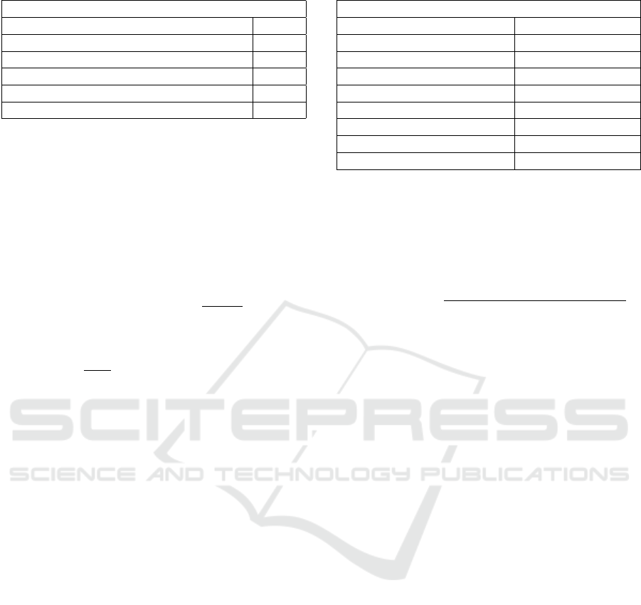
Table 3: Importance Factors in the Loss Function.

Loss Function Importance Factors for Voice VAE

Parameter Value

Reconstruction Importance 1

Sparsity Importance 0.3

Interpolation Importance 0.02

Disentanglement Importance of Speakers 0.25

Disentanglement Importance of Digits 0.25

voice of 6 speakers who have recorded the digits 0 to

9. Hence, to train this model we have assumed that

the latent space is 16 dimensional where the ﬁrst 6 di-

mensions store the data for each speaker, and the later

10 dimensions store the data for the digits. The speak-

ers are considered as cat0 and digits are considered as

cat1. For a more sophisticated dataset, we might have

more categories. For each category, the Disentangle-

ment Loss is calculated as Equation (5).

d, j

= Max(cat

6=i

1 + | f

(5)

Where in Equation (5), Max(cat

6=i

calculates

the maximum latent value for the unrelated latent di-

mensions and

1+| f

calculates the Loss for the related

latent dimension. Hence, if unrelated latent dimen-

sions have a high value the ﬁrst term will increase.

The second term on the other hand will decrease if

the related latent dimension has a high value. Hence,

minimizing this term will result in suppressed values

in unrelated dimensions while reinforcing the values

in the related dimensions in the latent space. This

Loss is calculated for each category (in this case for

the Speakers and Digits category) and the results are

summed up using a coefﬁcient.

In (2), the I

, I

and I

represents the importance

coefﬁcients of the Loss terms. Notice that I

and L

are denoted symbolically as one Loss term here but in

fact, it contains the Loss terms for two categories and

there are two importance coefﬁcients, one for each

category. Table 3 represents the importance coefﬁ-

cients used in the network training.

The network is trained in the beginning using only

the Reconstruction Loss and then in the later itera-

tions, other Loss terms are introduced. This is done to

make the system more stable and force it to converge

to an area that is proper from a reconstruction point of

view. The injection of new Loss term causes a spike in

the overall Loss. Because the network is not adopted

in accordance with the new Loss term. Hence, M

, M

, and M

multipliers are considered to smooth

the spikes in Loss Function as the iteration index in-

crease. These multipliers are equal to zero until a cer-

tain iteration that are denoted as Start Iterations and

they increase to 1 linearly according to Equation (6)

Table 4: Training iterations for Voice VAE.

Training Start/Stop Iterations for Voice VAE

Iteration of Loss Term Iteration Index

Reconstruction Start 1

Sparsity Start 6000

Sparsity Stop 6100

Interpolation Start 6500

Interpolation Start 6600

Disentanglement Start 6800

Disentanglement Start 7300

Overall Training Stop 10000

as the number of iterations increases and new Loss

terms are added. These multipliers stay steady at 1

once they reach a certain iteration and are denoted as

Stop Iteration. Table 4 represents the Start and Stop

Iterations for multipliers.

EachLossTerm

Interation

Current

− Iteration

Start

I ter ation

Stop

− Iteration

Start

(6)

The last coefﬁcients in the (2) are B

to B

. During

the training, it can be seen that for some Importance

coefﬁcient values in the Loss Function some of the

Loss terms increase in favor of other terms that de-

crease. It causes a divergence for some Loss terms

during the training. Although it results in the mini-

mization of the overall Loss Function, we are more

interested in the scenario in which all Loss terms de-

crease or are near to each other even though the over-

all decrease in Loss Function is lesser than the case

in which one Loss term increases considerably and

others decrease. Hence, once the Loss terms are cal-

culated after applying Importance coefﬁcients and in-

jection Multipliers, the obtained Loss terms are sorted

from max to min. Then for the maximum term, a co-

efﬁcient with a high value is applied, while for the

smaller Loss terms, a smaller coefﬁcient is applied.

This results in a schema in which the Loss term with

the highest value will have the highest importance to

decrease. However, once it is reduced enough such

that it becomes the second biggest Loss term, its im-

portance will be reduced for the optimizer, and hence

the optimizer does not continue to decrease this Loss

term with the cost of keeping other Loss terms in

higher values. Table 5 represents the coefﬁcients ap-

plied to lose terms according to their amplitude during

the training. Figure 3 represents the effect of applying

the B

coefﬁcient.

The reconstructed signal sample is depicted in

Figure 4. The audio signals are available on the

GitHub page of the paper (Solhjoo, b), (Solhjoo, a),

(Solhjoo, c).

Figure 5 and 6 represent the average value of the

Latent Code Disentanglement Using Orthogonal Latent Codes and Inter-Domain Signal Transformation

431

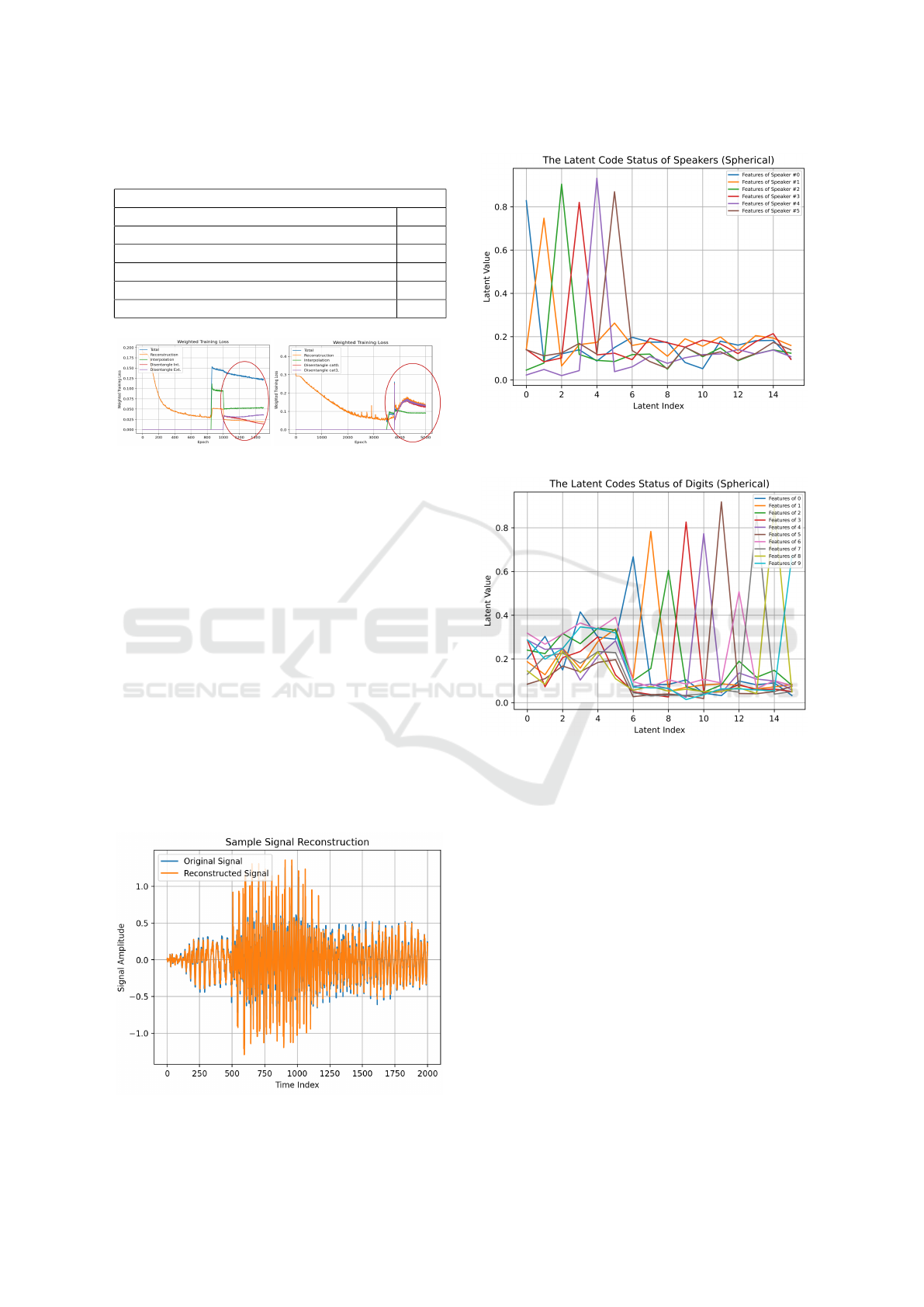
Table 5: Loss term Balancing Factors with respect to their

amplitude.

Loss Terms Balancing Coefﬁcients for Voice VAE

Maximum Loss Terms (Descending Order) Value

Max0 1

Max1 0.5

Max2 0.4

Max3 0.3

Max4 0.2

Figure 3: Left: Loss terms divergence without B

Factors;

Right: Loss terms convergence with B

Factors.

generated latent codes for different speakers and dig-

its respectively. To obtain these ﬁgures the latent

codes are normalized using the latent code amplitude.

Hence the dimension with the highest amplitude for

a feature implicitly means that most of the data are

encoded in that dimension. The ﬁgures represent the

proper disentanglement between the latent for differ-

ent features. Although the generated codes are not

exactly orthogonal they resemble this feature to a no-

ticeable extent.

3.2 Image Model

We also trained a model for digit images using the

MNIST-Image dataset. The methodology for train-

ing the image VAE is very similar to the one applied

in the Voice VAE. The only difference is in the fact

Figure 4: Sample voice signal reconstruction.

Figure 5: Average value of the latent codes for speakers in

Voice VAE.

Figure 6: Average value of the latent codes for the digits in

Voice VAE.

that the convolutional layers for the Voice VAE are 1-

dimensional while for Image VAE are 2-dimensional.

Table 6 represents the details of the convolutional lay-

ers for the Image VAE. In this network, each layer is

followed by a Relu Activation Function. In the last

layer of the decoder network, there is also a Sigmoid

Activation Function for the same reasons explained in

the voice model.

Table 7 represents the important Factors used in

Image VAE training. The MNIST-Image dataset

contains different digits with different hand-writings.

However, there is no detail about different writers.

Hence here it has been assumed that all digits are writ-

ten by a single writer. Accordingly, the latent space

for the Image-VAE is selected to be 11 dimensional

where 1 dimension is dedicated to the writer and 10

dimensions for the digits. Since there is only one

writer, it is already known that all writings belong to

ICAART 2023 - 15th International Conference on Agents and Artiﬁcial Intelligence

432

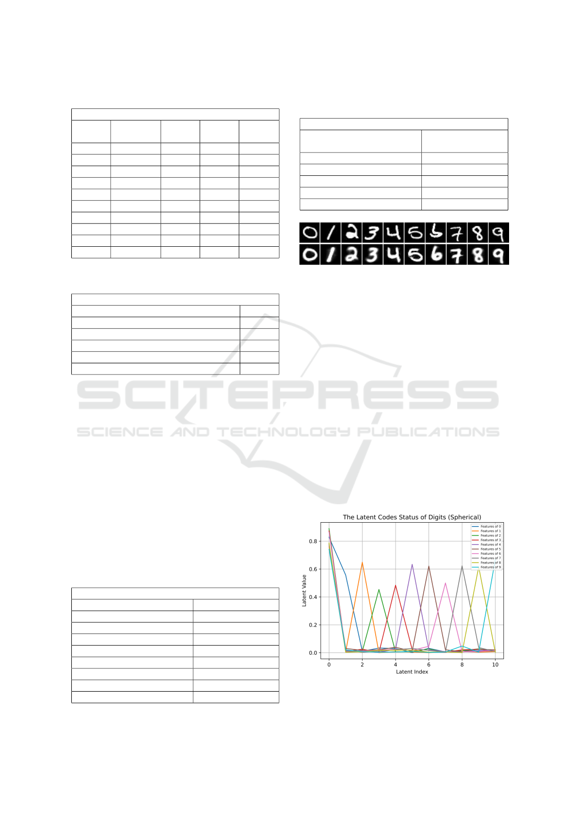
Table 6: Convolutional layer details for Image VAE.

Details of each convolutional layer for Image VAE

Layer

Index

Output

Channels

Kernels

Size

Stride Padding

L1 1012 7 2 1

L2 405 5 1 1

L3 162 3 1 1

L4 115 3 1 1

L5 82 3 1 1

L6 59 3 1 1

L7 42 3 1 1

L8 30 3 1 1

L9 21 3 1 1

L10 15 3 1 1

Table 7: Importance Factors in the Loss Function for Image

VAE.

Loss Function Importance Factors for Image VAE

Parameter Value

Reconstruction Importance 1

Sparsity Importance 0.3

Interpolation Importance 0.02

Disentanglement Importance of Writers 0

Disentanglement Importance of Digits 0.4

a speciﬁc writer and hence the Disentanglement Im-

portance Factor for the writer is selected to be zero.

The Image-VAE is trained for 800 iterations. The

Start and Stop Iterations for Loss terms in the Image-

VAE training are listed in Table 8.

The Loss terms Balancing Factors for Image VAE

are similar to Voice VAE and it is listed in Table 9.

The trained model performance for reconstructing

images is depicted for some samples in Figure 7.

The latent codes generated for different digits are

averaged and depicted in Figure 8. As depicted in the

ﬁgure the latent codes for digits are almost orthogonal

and separated. The latent code in the ﬁrst dimension

always has a high value as it represents the writer and

it was assumed that there is only one writer for all

digits.

Table 8: Training iterations for Image VAE.

Training Start/Stop Iterations for Image VAE

Iteration of Loss Term Iteration Index

Reconstruction Start 1

Sparsity Start 400

Sparsity Stop 410

Interpolation Start 450

Interpolation Start 460

Disentanglement Start 480

Disentanglement Start 530

Overall Training Stop 800

Table 9: Loss term Balancing Factors with respect to their

amplitude.

Loss Terms Balancing Coefﬁcients for Image VAE

Maximum Loss Terms By

Descending Order

Coefﬁcient

Value

Max0 1

Max1 0.5

Max2 0.4

Max3 0.3

Max4 0.2

Figure 7: Reconstructed images using the Image VAE.

Up row are the original images; below row are the recon-

structed images.

At this point, we have two networks that are able

to generate similar codes for the same features (for

instance digit 5) despite the fact that their data do-

mains are very different. Now if, for instance, the

character ”5” is associated with a code such as ”1-

0000010000” then this image can be generated in-

stantly. Hence, it can be observed that this method

provides an immediate possibility to generate the tex-

tual characters using latent codes and vice versa. Fig-

ure 9 represents the generated digits that are obtained

from the hand-crafted orthogonal codes such as ”1-

0000010000”. This should be noticed that the gener-

ated codes in the latent domains are not exactly 0 in

unrelated dimensions hence some imperfections can

be seen in these images speciﬁcally in digit 4. The

decoded images for hand-crafted codes presented in

Figure 9 aim to demonstrate that even an approxima-

Figure 8: Average value of the latent codes for the digits in

Image VAE.

Latent Code Disentanglement Using Orthogonal Latent Codes and Inter-Domain Signal Transformation

433

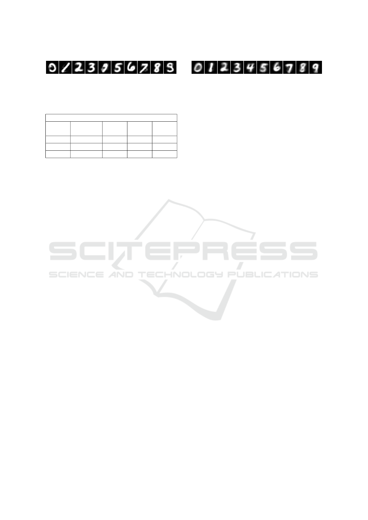
Figure 9: Image generation using handcrafted orthogonal

codes.

Table 10: Convolutional layer details for the bridge net-

work.

Details of each convolutional layer for Bridge Net

Layer

Index

Output

Channels

Kernels

Size

Stride Padding

L1 64 3 1 1

L2 64 3 1 1

L3 64 3 1 1

tion over the latent codes can generate acceptable out-

puts.

3.3 Inter-Domain Signal

Transformation: Voice to Image

Noting the fact that the latent codes obtained from dif-

ferent signal domains are very similar to each other

using the proposed method, we compose a hybrid

network in this section. This hybrid network takes

the encoder network of the Voice VAE and the de-

coder network of the Image VAE. The objective is to

generate an image using the related voice. The only

problem here is that the latent space for the Image

VAE is 11-dimensional while for Voice VAE is 16-

dimensional. Hence, we also create a thin bridge net-

work to map 16-dimensional space to 11 dimensions.

An alternative for this method is to simply remove the

speaker category section of the latent codes obtained

from the Voice VAE and only feed the digits part to

the image decoder. If this alternative approach is se-

lected, a high value (' 1) should be inserted in the

ﬁrst dimension of the crafted latent code in the writer

position since there is only one writer position in the

latent space.

The details of the bridge network designed for

mapping the voice latent to image latent are listed in

Table 10.

The bridge network is trained lightly using the

voice signals as the input of the Voice VAE encoder

and corresponding images in the output of the Image

VAE decoder. For training the bridge network, only

the Reconstruction Loss is considered. Figure 10 rep-

resents the sample results obtained from the conver-

sion of the voice signals to the images and it reﬂects

the fact that the conversion of the signal domain using

orthogonal encoding in the latent domain is possible

and provides acceptable results.

The hyper-parameters mentioned in Table 2 to Ta-

Figure 10: Images constructed from voice signals.

ble 10 are obtained empirically by training different

models and observing the results. To do so more than

100 models are trained for the Voice VAE. A similar

approach has been taken for Image and Bridge Net-

works. The enlisted parameters seem to provide bet-

ter audio-visual results.

4 CONCLUSIONS

In this work, we presented a method that is capable to

generate unique and orthogonal codes for the features

coming from different signal domains. This method

provides the possibility to train specialized networks

for different domains of data separately and then com-

bine their results in the latent domain. It is also rep-

resented that it is possible to create hybrid systems

using which the data can be transferred from one do-

main to another one. In this paper, we used voice,

image, and textual data domains to show the power of

this method and obtained acceptable results.

REFERENCES

Bank, D., Koenigstein, N., and Giryes, R. (2020). Autoen-

coders. arXiv preprint arXiv:2003.05991.

Cosmo, L., Norelli, A., Halimi, O., Kimmel, R., and

Rodol

a, E. (2020). LIMP: Learning latent shape rep-

resentations with metric preservation priors. In Com-

puter Vision – ECCV 2020, pages 19–35. Springer In-

ternational Publishing.

Guo, Y., Kasihmuddin, M. S. M., Gao, Y., Mansor, M. A.,

Wahab, H. A., Zamri, N. E., and Chen, J. (2022).

Yran2sat: A novel ﬂexible random satisﬁability logi-

cal rule in discrete hopﬁeld neural network. Advances

in Engineering Software, 171:103169.

Hopﬁeld, J.J., T. D. (1985). “neural” computation of deci-

sions in optimization problems. Biological Cybernet-

ics, 52:141–152.

Palash, M. H., Das, P. P., and Haque, S. (2019). Sentimental

style transfer in text with multigenerative variational

auto-encoder. In 2019 International Conference on

Bangla Speech and Language Processing (ICBSLP),

pages 1–4.

Pu, Y., Gan, Z., Henao, R., Yuan, X., Li, C., Stevens, A.,

and Carin, L. (2016). Variational autoencoder for deep

learning of images, labels and captions. In Lee, D.,

Sugiyama, M., Luxburg, U., Guyon, I., and Garnett,

R., editors, Advances in Neural Information Process-

ing Systems, volume 29, pages 2352–2360. Curran

Associates, Inc.

ICAART 2023 - 15th International Conference on Agents and Artiﬁcial Intelligence

434

Sadeghi, M. and Alameda-Pineda, X. (2020). Robust un-

supervised audio-visual speech enhancement using a

mixture of variational autoencoders. In ICASSP 2020

- 2020 IEEE International Conference on Acoustics,

Speech and Signal Processing (ICASSP), pages 7534–

7538.

Sadeghi, M., Leglaive, S., Alameda-Pineda, X., Girin, L.,

and Horaud, R. (2020). Audio-visual speech enhance-

ment using conditional variational auto-encoders.

IEEE/ACM Transactions on Audio, Speech, and Lan-

guage Processing, 28:1788–1800.

Solhjoo, R. https://github.com/babak-solhjoo/image-vae-

results.

Solhjoo, R. https://github.com/babak-solhjoo/voice-vae-

results.

Solhjoo, R. https://github.com/babak-

solhjoo/voice2imagevae.

Venkataramani, S., Tzinis, E., and Smaragdis, P. (2019). A

style transfer approach to source separation. In 2019

IEEE Workshop on Applications of Signal Processing

to Audio and Acoustics (WASPAA), pages 170–174.

Wang, Y., Hu, T., Wang, Z., Cai, J., and Du, H. (2018).

Hellinger distance based conditional variational auto-

encoder and its application in raw audio generation.

In 2018 IEEE 18th International Conference on Com-

munication Technology (ICCT), pages 75–79.

Wang, Y.-A., Huang, Y.-K., Lin, T.-C., Su, S.-Y., and Chen,

Y.-N. (2019). Modeling melodic feature dependency

with modularized variational auto-encoder. In ICASSP

2019 - 2019 IEEE International Conference on Acous-

tics, Speech and Signal Processing (ICASSP), pages

191–195.

APPENDIX

A pseudo-code for training a VAE with orthogonal la-

tent codes is presented below:

//Initializing M_i values

M_Reconstruction=1

M_Sparity=0

M_Interp=0

M_Disent=0

//Training over iterations

for Iteration in range(0,MaxIter):

//Signal normalization

Signal[l]=SignalBatchSampler()

SortedSig[l]=Sort(Signal)

NormFactor[l]=Average(SortedSig[l,0:M])

NormalizedSig[l]=Signal[l]/NormFactor[l]

//Encoding signal

PrimaryLatent[l]=Encoder(NormalizedSig[l])

//Normalize each category in latent code

for all categories in PrimaryLatent[l]:

{

NormCat[l,i]=L2Norm(Cat[l,i])

LatentCode[l]=

Concatination[Cat[l,i]/NormCat[l,i]]

}

//Resampling

SampStd[l]=LatentCode[l]*L+Std_min

LatentRe[l]=

Gaussian(SampStd[l], Latent[l])

//Decoding the signal

RecSignal[l]=Decoder(LatentRe[l])

//Output signal normalization

SortedRecSig[l]=Sort(RecSignal[l])

NormFactorRec[l]=Average(SortedSig[l,0:M])

NormRecSig[l]=RecSignal[l]/NormFactorRec[l]

//Calculating Reconstruction Loss

RecLoss[l]=

L2Norm(NormRecSig[l]-NormalizedSig[l])

//Calculating Sparsity Loss

SparsityLoss[l]=

L1Norm(NormRecSig[l]-NormalizedSig[l])

//Calculating Interpolation Loss

//Sampling and normalizing another signal

Signal[k]=SignalBatchSampler()

SortedSig[k]=Sort(Signal)

NormFactor[k]=Average(SortedSig[k,0:M])

NormalizedSig[k]=Signal[k]/NormFactor[k]

//Calculating latent code for the 2nd signal

PrimaryLatent[k]=Encoder(NormalizedSig[k])

//Normalize each category in latent code

for all categories in PrimaryLatent[k]:

{

NormCat[k,i]=L2Norm(Cat[k,i])

LatentCode[k]=

Concatination[Cat[k,i]/NormCat[k,i]]

}

//Sample a value with uniform distribution

Rand=UniformRandom()

//Combine signals in the time domain

MixedOrigSig[l]=

Rand*NormalizedSig[l]+

(1-Rand)*NormalizedSig[k]

//Combine latent codes of original signals

MixedLatent[l]=

Rand*LatentCode[l]+(1-Rand)*LatentCode[k]

//Resampling

SampStd[l]=MixedLatent[l]*L+Std_min

MixedLatentRe[l]=

Gaussian(SampStd[l], MixedLatent[l])

//Reconstructed signal from mixed latent

LatentMixedRecSig[l]=Decoder(MixedLatentRe[l])

Latent Code Disentanglement Using Orthogonal Latent Codes and Inter-Domain Signal Transformation

435

SortedMixRecSig[l]=Sort(LatentMixedRecSig[l])

NormFactorMixRec[l]=

Average(SortedMixRecSig[l,0:M])

NormMixRecSig[l]=

MixedRecSignal[l]/NormFactorMixRec[l]

//Calculating Interpolation Loss

InterpolLoss[l]=

L2Norm(MixedOrigSig[l]-NormMixRecSig[k])

//Calculating Disentanglement Loss

DisentangleLoss = 0

for all Cat in PrimaryLatent[l,n]:

{

UnrelatedDims=

Exclude(Related dimension in Cat)

PartialUnrelateLoss=Max(UnrelatedDims)

PartialRelatedLoss=1/(1+PrimaryLatent[l,n])

DisentangleLoss=

DisentangleLoss+PartialUnrelateLoss+

PartialRelatedLoss

}

//Calculating Mi multipliers

if(Iteration>SparsityStartIter and

Iteration<sparsityStopIter)

{

M_Sparity=(Iteration-SparsityStartIter)/

(SparsityStopIter-SparsityStartIter)

}

if(Iteration>=SparsityStopIter) M_Sparity=1

if(Iteration>InterpStartIter and

Iteration<InterpStopIter)

{

M_Interp=(Iteration-InterpStartIter)/

(InterpStopIter-InterpStartIter)

}

if(Iteration>=InterpStopIter) M_Interp=1

if(Iteration>DisentStartIter and

Iteration<DisentStopIter)

{

M_Disent=(Iteration-DisentStartIter)/

(DisentStopIter-DisentStartIter)

}

if(Iteration>=DisentStopIter) M_Disent=1

//Applying Mi to prioritize loss terms

LossTerms=Sort(RecLoss[l],SparsityLoss[l],

InterpolLoss[l],DisentangleLoss[l])

TotalLoss=WeightedSum(Bi*Mi*Ii*LossTerms)

Minimize TotalLoss by the backpropagating

gradient.

\section*{APPENDIX}

ICAART 2023 - 15th International Conference on Agents and Artiﬁcial Intelligence

436