Linking Data Separation, Visual Separation, and Classifier Performance
Using Pseudo-labeling by Contrastive Learning
B
´
arbara Caroline Benato
1 a
, Alexandre Xavier Falc
˜
ao
1 b
and Alexandru-Cristian Telea
2 c
1
Laboratory of Image Data Science, Institute of Computing, University of Campinas, Campinas, Brazil
2
Department of Information and Computing Sciences, Faculty of Science, Utrecht University, Utrecht, The Netherlands
Keywords:
Data Separation, Visual Separation, Semi-supervised Learning, Embedded Pseudo-labeling, Contrastive
Learning, Image Classification.
Abstract:
Lacking supervised data is an issue while training deep neural networks (DNNs), mainly when considering
medical and biological data where supervision is expensive. Recently, Embedded Pseudo-Labeling (EPL) ad-
dressed this problem by using a non-linear projection (t-SNE) from a feature space of the DNN to a 2D space,
followed by semi-supervised label propagation using a connectivity-based method (OPFSemi). We argue that
the performance of the final classifier depends on the data separation present in the latent space and visual
separation present in the projection. We address this by first proposing to use contrastive learning to produce
the latent space for EPL by two methods (SimCLR and SupCon) and by their combination, and secondly by
showing, via an extensive set of experiments, the aforementioned correlations between data separation, visual
separation, and classifier performance. We demonstrate our results by the classification of five real-world
challenging image datasets of human intestinal parasites with only 1% supervised samples.
1 INTRODUCTION
While supervised learning has achieved great suc-
cess, using datasets with either (i) few data points
or (ii) few supervised, i.e. labeled, points, is funda-
mentally hard, and especially critical in e.g. medi-
cal contexts where obtaining (labeled) points is ex-
pensive. For (i), methods such as few-shot learn-
ing (Sung et al., 2018; Sun et al., 2017), transfer-
learning (Russakovsky et al., 2015), and data aug-
mentation have been used to increase the sample
count. For (ii), solutions include semi-supervised
learning (Iscen et al., 2019; Wu and Prasad, 2018),
pseudo-labeling (Lee, 2013; Jing and Tian, 2020), and
meta-learning (Pham et al., 2021).
Pseudo-labeling, also called self-training, takes a
training set with few supervised and many unsuper-
vised samples and assigns pseudo-labels to the lat-
ter samples – a process known as data annotation –
and re-trains the model with all (pseudo)labeled sam-
ples. Yet, as the name suggests, pseudo-labels are not
perfect, as they are extrapolated from actual labels,
a
https://orcid.org/0000-0003-0806-3607
b
https://orcid.org/0000-0002-2914-5380
c
https://orcid.org/0000-0003-0750-0502
which can affect training performance (Benato et al.,
2018; Arazo et al., 2020). Also, pseudo-labeling
methods still require training and validation sets with
thousands of supervised samples per class to yield
reasonable results (Miyato et al., 2018; Jing and Tian,
2020; Pham et al., 2021).
Both pseudo-labeling, and broader, the success of
training a classifier, depend on a key aspect – how
easy is the data separable into different groups of
similar points. Projections, or dimensionality reduc-
tion methods, are well known techniques that aim to
achieve precisely this (Nonato and Aupetit, 2018; Es-
padoto et al., 2019). Two key observations were made
in this respect (discussed in detail in Sec. 2):
O1 Visual separability (VS) in a projection mimics
the data separability (DS) in the high dimen-
sional space;
O2 Data separability (DS) is key to achieving high
classifier performance (CP);
These observations have been used in several
directions, e.g., using projections to assess DS
(VS→DS) (der Maaten et al., 2009); using pro-
jections to find which samples get misclassified
(VS→CP) (Nonato and Aupetit, 2018); increasing DS
to get easier-to-interpret projections (DS→VS) (Kim
Benato, B., Falcão, A. and Telea, A.
Linking Data Separation, Visual Separation, and Classifier Performance Using Pseudo-labeling by Contrastive Learning.
DOI: 10.5220/0011856300003417
In Proceedings of the 18th International Joint Conference on Computer Vision, Imaging and Computer Graphics Theory and Applications (VISIGRAPP 2023) - Volume 5: VISAPP, pages
315-324
ISBN: 978-989-758-634-7; ISSN: 2184-4321
Copyright
c
 2023 by SCITEPRESS – Science and Technology Publications, Lda. Under CC license (CC BY-NC-ND 4.0)
315

et al., 2022b); using projections to assess classi-
fication difficulty (VS→CP) (Rauber et al., 2017a;
Rauber et al., 2017b); and using projections to build
better classifiers (VS→CP) (Benato et al., 2018; Be-
nato et al., 2021a). However, to our knowledge, no
work so far has explored the relationship between DS,
VS, and CP in the context of using pseudo-labeling
for machine learning (ML).
We address the above by studying how to gener-
ate a high DS using contrastive learning approaches
which have shown state-of-the-art results (Chen et al.,
2020; Grill et al., 2020; He et al., 2020; Khosla et al.,
2020) and have surpassed results of (self-and-semi-)
supervised methods and even known supervised loss
functions such as cross-entropy (Chen et al., 2020).
We compare two contrastive learning models (Sim-
CLR (Chen et al., 2020) and SupCon (Khosla et al.,
2020)) and propose a hybrid approach that combines
both. We evaluate DS by measuring CP for a classi-
fier trained with only 1% supervised samples. Then,
we evaluate VS fed with the encoder’s output of our
trained contrastive models. Lastly, we investigate CP
by using our above pseudo-labeling to train a deep
neural network. We perform all our experiments in
the context of a challenging medical application (clas-
sifying human intestinal parasites in microscopy im-
ages).
Our main contributions are as follows:
C1: We use contrastive learning to reach high DS;
C2: We show that projections constructed from con-
trastive learning methods (with good DS) lead to
a good VS between different classes;
C3: We train classifiers with pseudo-labels generated
via good-VS projections to achieve a high CP.
Jointly taken, our work brings more evidence
that links the observations O1 and O2 mentioned
above, i.e., that VS, DS, and CP are strongly cor-
related and that this correlation, and 2D projections
of high-dimensional data, can be effectively used to
build higher-CP classifiers for the challenging case
of training-sets having very few supervised (labeled)
points.
2 RELATED WORK
Self-supervised Learning. Self-supervised con-
trastive methods in representation learning have been
the choice for learning representations without using
any labels (Chen et al., 2020; Grill et al., 2020; He
et al., 2020; Khosla et al., 2020). Such methods work
by using a so-called contrastive loss to pull similar
pairs of samples closer while pushing apart dissimi-
lar pairs. To select (dis)similar samples without using
label information, one can generate multiple views of
the data via transformations. For image data, Sim-
CLR (Chen et al., 2020) used transformations such as
cropping, Gaussian blur, color jittering, and grayscale
bias. MoCo (He et al., 2020) explored a momentum
contrast approach to learn a representation from a pro-
gressing encoder while increasing the number of dis-
similar samples. BYOL (Grill et al., 2020) used only
augmentations from similar examples. SimCLR has
shown significant advances in (self-and-semi-) super-
vised alearning and achieved a new record for im-
age classification with few labeled data. Supervised
contrastive learning (SupCon) (Khosla et al., 2020)
generalized both SimCLR and N-pair losses and was
proven to be closely related to triplet loss. SupCon
surpasses cross-entropy, margin classifiers, and other
self-supervised contrastive learning techniques.
Pseudo-labeling. An alternative to building accu-
rate and large training sets is to propagate labels from
a few supervised samples to a large set of unsuper-
vised ones by creating pseudo-labels. (Lee, 2013)
trained a neural network with 100 to 3000 supervised
images and then assigned the class with maximum
predicted probability to the remaining unsupervised
ones. The network is then fine-tuned using both true
and pseudo-labels to yield the final model. Yet, this
method requires a validation set with over 1000 super-
vised images to optimize hyperparameters. The same
issue happens for other pseudo-labeling strategies that
need a validation set (Miyato et al., 2018; Jing and
Tian, 2020; Pham et al., 2021).
Structure in (Embedded) Data. Data structure,
also called data separability (DS) is an accepted, al-
beit not formally, defined term in ML. Simply put,
for a dataset D = {x
i
|x
i
∈ R
n
}, DS refers to the pres-
ence of groups of points which are similar and also
separated from other point groups. DS is essential in
ML, especially classification. Obviously, the stronger
DS is, the easier is to build a classifier that separates
points belonging to the various groups with high clas-
sifier performance (CP). CP can be measured by many
metrics, e.g., accuracy, F1 score, or AUROC (Hossin
and Sulaiman, 2015). Indeed, if different-class points
are not separated via their features (coordinates in
R
n
), then no (or poor) classification (CP) is possible.
Projections, or Dimensionality Reduction (DR)
methods, take a dataset D and produce a scatterplot,
or embedding of D, P(D) = {y
i
= P(x
i
)|y
i
∈ R
q
},
where typically q ∈ {2, 3}. The aim is that the vi-
sual structure, also called visual separability (VS) in
VISAPP 2023 - 18th International Conference on Computer Vision Theory and Applications
316

P(D), literally seen in terms of point clusters sepa-
rated by whitespace, mimics DS. Many methods have
been proposed for P, with accompanying metrics to
gauge how much VS captures DS (Nonato and Au-
petit, 2018; Espadoto et al., 2019).
Relations between VS, DS, and CP have been par-
tially explored. (Rauber et al., 2017a) used the VS of
a t-SNE (van der Maaten, 2014) projection to gauge
the difficulty of a classification task (CP). They found
that VS and CS are positively correlated when VS is
medium to high but could not infer actionable insights
for low-VS projections. Also, they did not address the
task of building higher-CP classifiers using t-SNE. In
a related vein, (Rodrigues et al., 2019) used the VS
in projections to construct so-called decision bound-
ary maps to interpret classification performance (CP)
but did not actually use these to improve classifiers.
(Kim et al., 2022b; Kim et al., 2022a) showed that
one can improve VS by increasing DS, the latter be-
ing done by mean shift (Comaniciu and Meer, 2002).
However, their aim was to generate easier-to-interpret
projections and not use these to build higher-CP clas-
sifiers. Moreover, their approach actually changed
the input data in ways not easy to control, which
raises question as to the interpretability of the result-
ing projections. Next, (Benato et al., 2018; Benato
et al., 2021b) used the VS of t-SNE projections to cre-
ate pseudo-labels and train higher-CP classifiers from
them. They showed that label propagation in the 2D
projection space can lead to higher-CP classifiers than
when propagating labels in the data space. Yet, they
did not study how correlations between DS and VS
can affect CP.
Embedded Pseudo-Labeling (EPL). The above-
mentioned topics of pseudo-labeling and VS-CP
correlation were connected recently by Embedded
Pseudo-Labeling (EPL) (Benato et al., 2018), a
method proposed to increase the number of labeled
samples from only dozens of supervised samples,
without needing validation sets with more supervised
samples. To do this, EPL projects to 2D the latent
feature space extracted from a deep neural network
(DNN) using autoencoders (Benato et al., 2021b)
and pre-trained architectures (Benato et al., 2021a).
Pseudo-labels are next propagated in the 2D projec-
tion from supervised to unsupervised samples using
the OPFSemi (Amorim et al., 2016) method. How-
ever, the success of EPL strongly depends on the VS
in the projection space.
3 PROPOSED PIPELINE
Following the above, we propose to improve DS in
the feature space that EPL takes as input by us-
ing two contrastive learning models (SimCLR (Chen
et al., 2020) and SupCon (Khosla et al., 2020), used
both separately and combined) and without using
ground-truth labels. The feature space to input in
EPL comes from the encoder’s output from these
contrastive models. During the process, outlined in
Fig. 1, we test our three claims (Sec. 1), i.e., that DS
has improved (C1); that this has led to an improved
VS in the 2D projections used by EPL (C2); and fi-
nally that the generated pseudo-labels by EPL can
be used to train a classifier with high CP (C3). Our
method is detailed next.
image
transformations
parasite
images
encoder
linear
layers
dimensionality
reduction
label
estimation
pseudo-
labels
contrastive learning
pseudo-labeling by EPL
encoded features
classifier design
train
classifier
test
classifier
C3
C1
C2
2D projection
classifier
quality
good DS
good VS
good CP
flip, crop, jitter, ...
VGG-16
t-SNE OPFSemi
ResNet-18
contrastive loss
minimization
Figure 1: We train a model from image transformations of
the original data with a contrastive learning loss. Next, we
project the latent features from the encoder’s output to 2D
and pseudo-label the resulting points. Finally, we use these
pseudo-labels to train a classifier.
3.1 Contrastive Learning
We generate the latent space to be used by EPL
(Fig. 1, top box) in three different ways: (a) from the
many unsupervised samples available by using Sim-
CLR (Chen et al., 2020); (b) using our 1% supervised
samples with SupCon (Khosla et al., 2020); and (c) by
combining the SimCLR and SupCon methods.
3.2 Pseudo-labeling by EPL
Both SimCLR and SupCon use ResNet-18 (He et al.,
2016) as encoder. We reduce the output of ResNet-18
(hundreds of dimensions) to 2D using t-SNE (Fig. 1,
middle box). This is similar to EPL, which has shown
that propagating pseudo-labels in this 2D space cre-
ates large labeled training-sets that lead to high-CP
classifiers (Benato et al., 2021a; Benato et al., 2021c).
We use the 2D projection to propagate the (few) true
labels to all unsupervised points as in EPL. That
Linking Data Separation, Visual Separation, and Classifier Performance Using Pseudo-labeling by Contrastive Learning
317

is, we use OPFSemi (Amorim et al., 2016) which
maps (un)supervised samples to nodes of a complete
graph, with edges weighted by the Euclidean dis-
tance between samples. The cost of a path con-
necting two nodes is the maximal edge-weight on
that path. OPFSemi uses this graph to compute an
optimum-path forest of minimum-cost paths rooted
in the supervised samples. Each supervised sam-
ple assigns its label to its most closely connected
unsupervised nodes. OPFSemi was shown to per-
fom better for pseudo-label propagation than earlier
semi-supervised methods (Amorim et al., 2016; Be-
nato et al., 2018; Amorim et al., 2019).
3.3 Classifier Training with
Pseudo-labels
To finally test the quality of our generated pseudo-
labels, we train a deep neural network, namely VGG-
16 with ImageNet pre-trained weights, and test it on
our parasite datasets (Fig. 1, bottom box). This ar-
chitecture was shown to have the best results for our
datasets (Osaku et al., 2020).
4 EXPERIMENTS AND RESULTS
4.1 Datasets
As outlined in Sec. 1, we apply our proposed ap-
proach in the medical context. Our data (see Tab. 1)
consists of five image datasets of Brazil’s most com-
mon species of human intestinal parasites which are
responsible for public health problems and death in
infants and immunodeficient individuals in most trop-
ical countries (Suzuki et al., 2013). The first three
datasets contain color microscopy images of 200 ×
200 pixels: (i) Helminth larvae (H.larvae, 2 classes,
3,514 images); (ii) Helminth eggs (H.eggs, 9 classes,
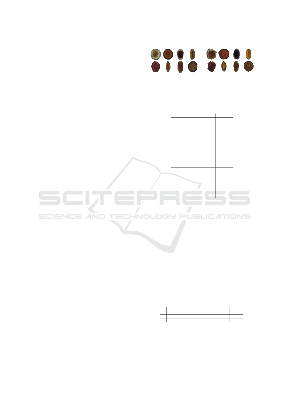
5,112 images, see examples in Fig. 2); and (iii) Pro-
tozoan cysts (P.cysts, 7 classes, 9,568 images). These
datasets are unbalanced and they also contain an im-
purity (adversarial) class that is very similar to the
parasite classes, making the problem even more chal-
lenging. To evaluate different difficulty levels, we
also explore (ii) and (iii) without the impurity class,
which form our last two datasets.
4.2 Experimental Setup
As outlined in Sec. 1, we aim to build a classifier for
our image data using a very small set of supervised
samples. For this, we split each of the five considered
Figure 2: H.eggs dataset. Left: images of parasites of the
eight classes in this dataset. Right: Corresponding images
of the impurities for each of the left classes which jointly
form class 9 (impurities).
Table 1: Parasites datasets. The class names, number of
classes, and number of samples per class are presented.
dataset classes # samples
(i) H.larvae
(2 classes)
S.stercoralis 446
impurities 3068
total 3,514
(ii) H.eggs
(9 classes)
H.nana 348
H.diminuta 80
Ancilostomideo 148
E.vermicularis 122
A.lumbricoides 337
T.trichiura 375
S.mansoni 122
Taenia 236
impurities 3,444
total 5,112
(iii) P.cysts
(7 classes)
E.coli 719
E.histolytica 78
E.nana 724
Giardia 641
I.butschlii 1,501
B.hominis 189
impurities 5,716
total 9,568
datasets D (Sec. 4.1) into a supervised training-set S
containing 1% supervised samples from D, an unsu-
pervised training-set U with 69% of the samples in D,
and a test set T with 30% of the samples in D (hence,
D = S ∪U ∪ T ). We repeat the above division ran-
domly and in a stratified manner to create three dis-
tinct splits of D in order to gain statistical relevance
when evaluating results next.
Table 2 shows the sizes |S| and |U| for each
dataset. To measure quality, we compute accuracy
(number of correct classified or labeled samples over
all the samples in a set) and Cohen’s κ (since our
datasets are unbalanced). κ gives the agreement level
between two distinct predictions in a range [−1,1],
where κ ≤ 0 means no possibility, and κ = 1 means
full possibility, of agreement.
Table 2: Number of samples in S and U for each dataset.
H.eggs
(w/o imp)
P. cysts
(w/o imp)
H. larvae H. eggs P. cysts
S 17 38 35 51 95
U 1220 2658 2424 3527 6602
4.3 Implementation Details
We next outline our end-to-end implementation.
VISAPP 2023 - 18th International Conference on Computer Vision Theory and Applications
318

Contrastive Learning: We implemented SimCLR
and SupCon in Python using Pytorch. We gener-
ate two augmented images (views) for each origi-
nal image by random horizontal flip, resized crop
(96×96), color jitter (brightness= 0.5, contrast= 0.5,
saturation= 0.5, hue= 0.1) with probability of 0.8,
gray-scale with probability of 0.2, Gaussian blur (9×
9), and a normalization of 0.5.
Latent Space Generation: We replace ResNet-
18’s decision layer by a linear layer with 4,096 neu-
rons, a ReLU activation layer, and a linear layer
with 1,024 neurons respectively. We train the model
by backpropagating errors of NT-Xent and SupCon
losses for SimCLR and SupCon, respectively, with a
fixed temperature of 0.07. We use the AdamW op-
timizer with a learning rate of 0.0005, weight decay
of 0.0001, and a learning rate scheduler using cosine
annealing, with a maximum temperature equal to the
epochs and minimum learning rate of 0.0005/50. We
use 50 epochs and select the best model through a
checkpoint obtained from the lowest validation loss
during training. Finally, we use the 512 features of
the ResNet-18’s encoder to obtain our latent space.
Classifier Using Pseudo-labels: We replace the
original VGG-16 classifier with two linear layers with
4,096 neurons followed by ReLU activations and a
softmax decision layer. We train the model with the
last four layers unfixed by backpropagating errors us-
ing categorical cross-entropy. We use stochastic gra-
dient descent with a linear decay learning rate initial-
ized at 0.1 and momentum of 0.9 over 15 epochs.
Parameter Setting: OPFSup and OPFSemi, used
for pseudo-labeling (Sec. 3.2), have no parameters.
For Linear SVM and t-SNE (Sec. 4.4.1), we use the
default parameters provided by scikit-learn.
For replication purposes, all our code and results
are made openly available (Benato, B.C., 2022).
4.4 Proposed Experiments
To describe our experiments, we first introduce a few
notations. S, U, and T are the supervised (known la-
bels), unsupervised (to be pseudo-labeled), and test
sets (see Sec. 4.2). Let I be the images in a given
dataset having true labels L and pseudo-labels P. Let
F be the latent features obtained by the three con-
trastive learning methods; and let F
′
be the features’
projection to 2D via t-SNE. We use subscripts to de-
note on which subset I, L, P, and F are computed, e.g.
F
S
are the latent features for samples in S. Finally, let
A be the initialization strategy for training a classifier
C.
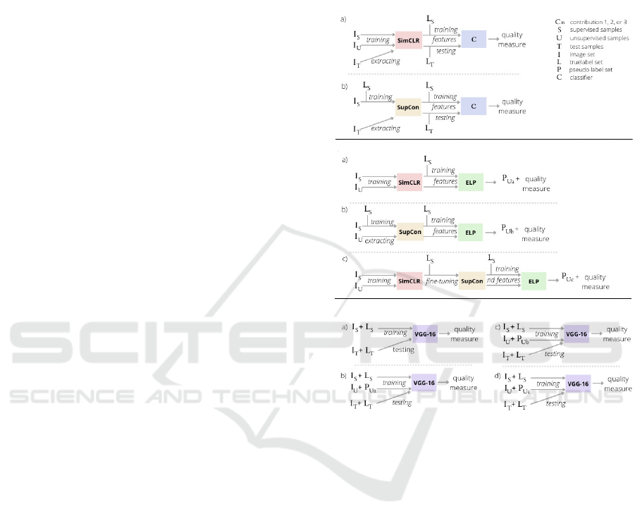
Figure 3 shows the several experiments we exe-
cuted to explore the claims C1-C3 listed in Sec. 1.
These experiments are detailed next.
nD
nD
nD
nD
C1
C2
C3
Legend
Figure 3: Summary of the proposed experiments.
4.4.1 Testing C1
Our claim C1 is that contrastive learning methods pro-
duce high separability of classes (i.e., DS) in the pro-
duced feature space. Also, our using of contrastive
learning has increased propagation accuracy by up to
20% vs using a simpler method, i.e., generating the la-
tent space via autoencoders (Benato et al., 2018). Di-
rectly measuring DS is hard since the concept of data
separability is not uniquely and formally defined (see
Sec. 2). As such, we assess DS by a ‘proxy’ method:
We train two distinct classifiers C, both using 1% su-
pervised samples. These are Linear SVM, a simple
linear classifier used to check the linear separability
of classes in the latent space; and OPFSup (Papa and
Falc
˜
ao, 2009), an Euclidean distance-based classifier.
If these classifiers yield high quality, it means that DS
is high, and conversely. We measure quality by clas-
sifier accuracy and κ over correctly classified samples
in T .
With the above, we execute two experiments – one
Linking Data Separation, Visual Separation, and Classifier Performance Using Pseudo-labeling by Contrastive Learning
319

per method of latent space generation (see Sec. 3.1):
a) SimCLR: Train with A on I
S∪U
; extract features
F
S
and F
T
; train C on F
S
and L
S
; test on F
T
and
L
T
.
b) SupCon: Train with A on I
S
and L
S
; extract fea-
tures F
S
and F
T
; train and test as above.
4.4.2 Testing C2
Similarly to C1, evaluating the VS of projections to
test C2 can be done in many ways since visual sepa-
ration of clusters in a 2D scatterplot is a broad con-
cept. In DR literature, several metrics have been
proposed for this task (see surveys (Espadoto et al.,
2019; Nonato and Aupetit, 2018)). Yet, such met-
rics are typically used to gauge the projection quality
when explored by a human. Rather, in our context,
we use projections automatically to drive pseudo-
labeling and improve classification (Sec. 3.2). As
such, it makes sense to evaluate our projections’ VS
by how well they can do this label propagation. For
this, we compare the computed pseudo-labels with the
true, supervised, labels by computing accuracy and κ
for the correctly computed pseudo-labels over U. We
do this via three experiments:
a) SimCLR: Train with A on I
S∪U
; extract features
F
S∪U
; compute 2D features F
′
with t-SNE from
F
S∪U
; propagate labels L
S
with OPFSemi from
F
′
S
to F
′
U
;
b) SupCon: Train with A on I
S
and L
S
; extract fea-
tures F
S∪U
; compute 2D features F
′
with t-SNE
from F
S∪U
; propagate labels as above;
c) SimCLR+SupCon: Train SimCLR with A on
I
S∪U
; fine-tune with SupCon on I
S
and L
S
; ex-
tract features I
S∪U
; compute 2D features F
′
with
t-SNE from F
S∪U
; propagate labels as above.
4.4.3 Experiments for Testing C3
Finally, we use the computed pseudo-labels to train
and test a DNN classifier, namely VGG-16, to test C3,
i.e., gauge how CS is correlated (or not) with VS and
DS. For this, we do the following experiments:
a) baseline: train with I
S
and L
S
; test on I
T
and L
T
;
b) SimCLR: train with I
S∪U
and L
S∪P
U
, with
pseudo-labels P
U
from (Sec. 4.4.2,a); test as
above;
c) SupCon: train with I
S∪U
and L
S∪P
U
, with pseudo-
labels P
U
from (Sec. 4.4.2,b); test as above;
d) SimCLR+SupCon: train with I
S∪U
and L
S∪P
U
,
with pseudo-labels P
U
from (Sec. 4.4.2,c); test
as above.
4.5 Results
We present the results of the experiments in Sec. 4.4
and along our claims C1-C3.
4.5.1 C1: Contrastive Learning Yields High DS
Table 3 shows the classification results for the experi-
ments in Sec. 4.4.1 in terms of accuracy and κ (mean
and standard deviation) for the trained Linear SVM
and OPFSup classifiers.
We first discuss the contrastive learning methods
trained from scratch vs using ImageNet pre-trained
weights. For all datasets, the best accuracy and κ
exceed 0.70 and 0.50 respectively. Linear SVM ob-
tained the best results, showing that the tested latent
spaces have a reasonable linear separation between
classes even when classified with only 1% supervised
samples. In contrast, OPFSup seems to suffer from
the dimensionality curse as it uses Euclidean dis-
tances in the latent space. This further motivates the
latent space’s dimensionality reduction when using
an OPF classifier. Separately, we see that SimCLR
was helped by the ImageNet pre-trained weights,
while SupCon obtained its best results when trained
from scratch for datasets with impurities. SimCLR
had an increase of around 0.10 in accuracy and κ
for H.eggs and P.cysts without impurities with pre-
trained weights. SupCon also had an extra 0.10 accu-
racy and κ for datasets with impurities when trained
from scratch. Since SupCon achieved its best results
from scratch and SimCLR was helped by pre-trained
weights for distinct datasets, we next explore the com-
bination of both methods.
4.5.2 C2: Projections of Contrastive Latent
Spaces Yield High VS
Table 4 show the results for the experiments in
Sec. 4.4.2, i.e., the mean propagation accuracy and κ
in pseudo-labeling for the correctly assigned labels in
U for EPL run on latent spaces created by SimCLR,
SupCon, and SimCLR+SupCon.
The best results were obtained when using the
ImageNet pre-trained weights. This shows that the
pseudo-labeling on the contrastive latent space is fa-
vored by such pre-trained weights. SupCon gained
almost 0.20 in κ compared with SimCLR for H.eggs
and P.cysts without impurity. SupCon obtained the
best results for the H.Eggs and P.cysts without impu-
rities, while the SimCLR+SupCon obtained the best
results for the same datasets with impurities. Sim-
CLR+SupCon improved the results of SimCLR for
those datasets. For H.larvae, the results of the three
methods were similar.
VISAPP 2023 - 18th International Conference on Computer Vision Theory and Applications
320

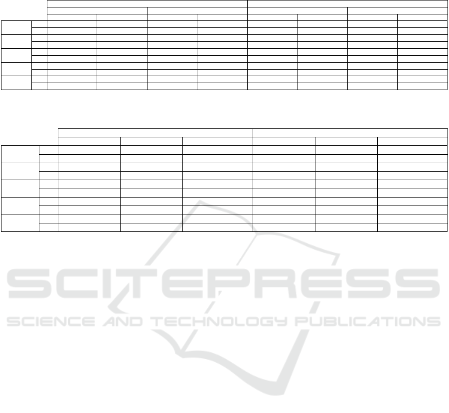
Table 3: C1: DS assessment of SimCLR’s and SupCon’s latent spaces using Linear SVM and OPFSup on T. Both methods
are compared trained from scratch and with pre-trained weights during 50 epochs. Best values per dataset are in bold.
trained from scratch with ImageNet pre-trained weights
a) SimCLR b) SupCon a) SimCLR b) SupCon
Linear SVM OPFSup Linear SVM OPFSup Linear SVM OPFSup Linear SVM OPFSup
H.eggs
(w/o imp)
acc 0.814606 ± 0.079 0.759631 ± 0.107 0.863954 ± 0.064 0.858565 ± 0.057 0.903327 ± 0.021 0.869429 ± 0.033 0.789705 ± 0.042 0.817326 ± 0.047
κ 0.668252 ± 0.091 0.585225 ± 0.098 0.778473 ± 0.029 0.742304 ± 0.106 0.884889 ± 0.025 0.844527 ± 0.04 0.750924 ± 0.049 0.783428 ± 0.056
P.cysts
(w/o imp)
acc 0.637543 ± 0.177 0.632065 ± 0.017 0.717705 ± 0.022 0.643310 ± 0.045 0.771627 ± 0.019 0.706747 ± 0.038 0.675606 ± 0.056 0.580450 ± 0.006
κ 0.547758 ± 0.168 0.523332 ± 0.02 0.615566 ± 0.025 0.529749 ± 0.053 0.689346 ± 0.027 0.605509 ± 0.049 0.564481 ± 0.061 0.443273 ± 0.015
H.larvae
acc 0.901106 ± 0.025 0.888784 ± 0.011 0.933649 ± 0.011 0.905845 ± 0.033 0.950079 ± 0.006 0.947551 ± 0.008 0.952923 ± 0.007 0.946287 ± 0.008
κ 0.381798 ± 0.233 0.422084 ± 0.037 0.711252 ± 0.069 0.539386 ± 0.237 0.767091 ± 0.041 0.751936 ± 0.054 0.782983 ± 0.053 0.756410 ± 0.054
H.eggs
acc 0.542590 ± 0.177 0.575185 ± 0.014 0.789222 ± 0.028 0.756410 ± 0.035 0.758800 ± 0.053 0.736202 ± 0.029 0.761191 ± 0.071 0.743590 ± 0.069
κ 0.126531 ± 0.046 0.279272 ± 0.023 0.626696 ± 0.037 0.592371 ± 0.039 0.529617 ± 0.125 0.521839 ± 0.056 0.588783 ± 0.111 0.567762 ± 0.095
P.cysts
acc 0.563335 ± 0.045 0.541159 ± 0.018 0.722048 ± 0.009 0.609544 ± 0.019 0.674678 ± 0.064 0.604551 ± 0.023 0.628701 ± 0.168 0.649483 ± 0.05
κ 0.330526 ± 0.031 0.288527 ± 0.012 0.525391 ± 0.045 0.370582 ± 0.022 0.422320 ± 0.112 0.375311 ± 0.037 0.441970 ± 0.168 0.429321 ± 0.065
Table 4: C2: Propagation results for pseudo-labeling U on the projected SimCLR’s and SupCon’s latent spaces, from scratch
and using ImageNet pre-trained weights. Best values per dataset are in bold.
trained from scratch with ImageNet pre-trained weights
a) SimCLR b) SupCon c) SimCLR+SupCon a) SimCLR b) SupCon c) SimCLR+SupCon
H.eggs
(w/o imp)
acc 0.861493 ± 0.012 0.713554 ± 0.077 0.896255 ± 0.041 0.795203 ± 0.129 0.951765 ± 0.041 0.830234 ± 0.123
κ 0.561568 ± 0.009 0.473379 ± 0.025 0.567093 ± 0.020 0.756312 ± 0.153 0.942519 ± 0.049 0.797482 ± 0.148
P.cysts
(w/o imp)
acc 0.652324 ± 0.027 0.641073 ± 0.038 0.650470 ± 0.027 0.568991 ± 0.036 0.706973 ± 0.092 0.565282 ± 0.091
κ 0.537704 ± 0.043 0.531090 ± 0.040 0.533208 ± 0.031 0.428962 ± 0.036 0.619738 ± 0.102 0.439581 ± 0.103
H.larvae
acc 0.898739 ± 0.033 0.886539 ± 0.003 0.941169 ± 0.013 0.959062 ± 0.007 0.946184 ± 0.010 0.954724 ± 0.005
κ 0.532710 ± 0.179 0.404983 ± 0.119 0.694591 ± 0.029 0.817274 ± 0.030 0.777621 ± 0.020 0.792838 ± 0.009
H.eggs
acc 0.710173 ± 0.035 0.585802 ± 0.026 0.741755 ± 0.065 0.719862 ± 0.077 0.751723 ± 0.052 0.780418 ± 0.080
κ 0.357514 ± 0.044 0.178536 ± 0.031 0.374099 ± 0.108 0.532788 ± 0.120 0.553654 ± 0.094 0.624724 ± 0.113
P.cysts
acc 0.607884 ± 0.049 0.530785 ± 0.019 0.666119 ± 0.027 0.670898 ± 0.051 0.577025 ± 0.049 0.705042 ± 0.035
κ 0.380969 ± 0.066 0.235849 ± 0.018 0.457391 ± 0.056 0.430201 ± 0.022 0.320479 ± 0.057 0.513962 ± 0.043
4.5.3 C3: Classifiers Trained by Pseudo-labels
obtained from High-VS Projections have a
High CP
Table 5 shows the results of classification for VGG-
16 trained from the pseudo-labeling performed on
latent spaces from SimCLR, SupCon, and Sim-
CLR+SupCon.
We notice that the results of VGG-16’s classifica-
tion follow the same pattern as the propagation results
(Tab. 4). The best results were found by the methods
using the ImageNet pre-trained weights. Also, Sup-
Con obtained the best results for H.Eggs and P.cysts
without impurities, while SimCLR+SupCon obtained
the best results for the same datasets with impurities.
SupCon showed a gain of almost 0.20 in κ for H.eggs
without impurity and H.larvae, and 0.15 for P.cysts
without impurity when compared with the baseline.
In short, the results show that VGG-16 can learn from
the pseudo-labels since it provided good classification
accuracies and κ – higher than 0.85 and 0.76, respec-
tively – for H.eggs and P.cysts without impurity and
H.Larvae. However, the compared methods could not
surpass the baseline for H.eggs and P.cysts with im-
purities. We discuss this aspect next.
5 DISCUSSION
We next discuss several aspects pertaining to our re-
sults.
5.1 Visual Separation vs Classifier
Performance
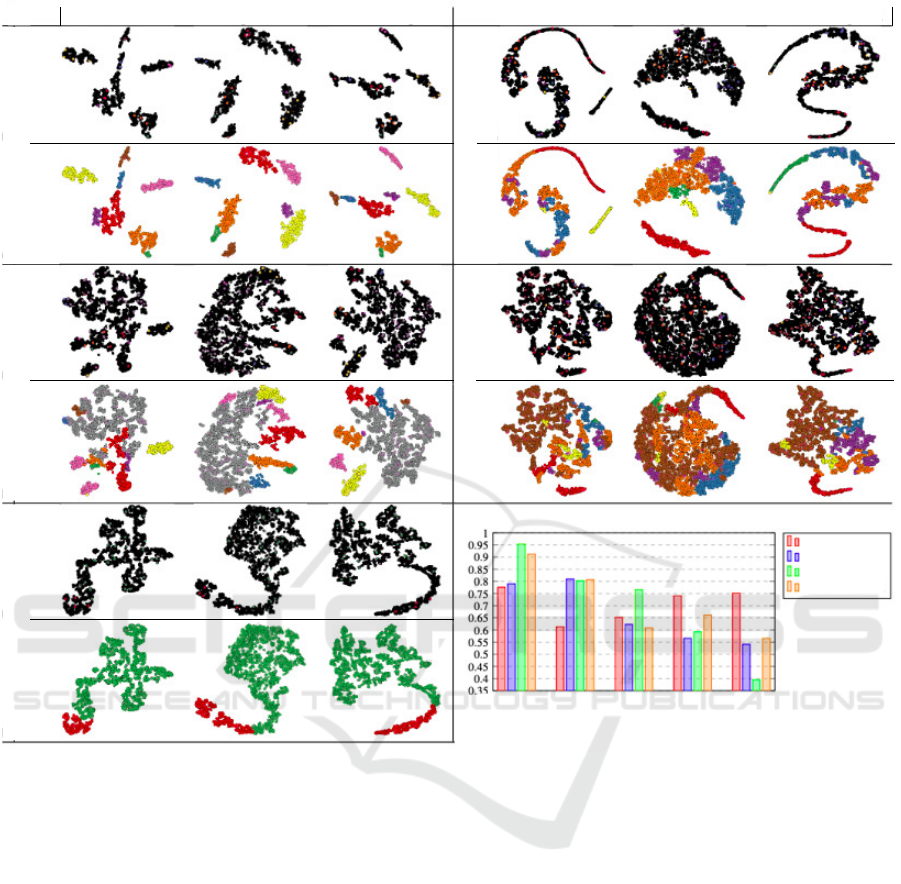
Figure 4.i shows the 2D t-SNE projections of the three
computed latent spaces for all five studied datasets.
For each dataset, the top row (a) shows the few
(1%) supervised labels (colored points) thinly spread
among the vast majority of unsupervised (black) sam-
ples; the bottom row (b) shows samples colored by the
computed pseudo-labels.
We see in all images a good correlation of the
visual separation VS (point groups separated from
each other by whitespace) with the lack of label mix-
ing in such groups. For H.eggs without impurity, all
three latent space projections show a clear VS, and
we see that this leads to almost no color mixing in
the propagated pseudo-labels. For the H.eggs dataset,
we see how the visually separated groups show al-
most no color mixing, whereas the parts of the projec-
tion where no VS is present show color mixing. For
P.cysts without impurity, there is a clearly separated
group at the bottom in all three projections which
also has a single color (label). The remaining parts of
the projections, which have no clear VS into distinct
Linking Data Separation, Visual Separation, and Classifier Performance Using Pseudo-labeling by Contrastive Learning
321

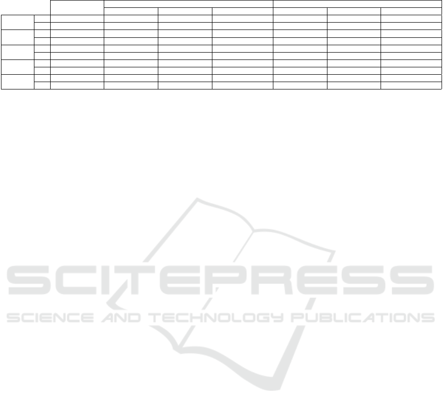
Table 5: C3: VGG-16’s classification results on T when using pseudo labels from SimCLR’s, SupCon and SimCLR+SupCon
latent spaces, from scratch and with ImageNet pre-trained weights. Best values per dataset are in bold.
a) baseline
trained from scratch with ImageNet pre-trained weights
b) SimCLR c) SupCon d) SimCLR+SupCon a) SimCLR b) SupCon c) SimCLR+SupCon
H.eggs
(w/o imp)
acc 0.812932 ± 0.059 0.435028 ± 0.400 0.714375 ± 0.088 0.925926 ± 0.035 0.823603 ± 0.138 0.961080 ± 0.039 0.858129 ± 0.127
κ 0.775954 ± 0.073 0.292310 ± 0.506 0.662603 ± 0.098 0.912482 ± 0.041 0.790296 ± 0.164 0.953710 ± 0.047 0.831107 ± 0.152
P.cysts
(w/o imp)
acc 0.757209 ± 0.015 0.589965 ± 0.174 0.662053 ± 0.064 0.606113 ± 0.188 0.752905 ± 0.183 0.857411 ± 0.085 0.740945 ± 0.216
κ 0.651933 ± 0.023 0.383736 ± 0.334 0.558104 ± 0.071 0.408416 ± 0.354 0.622887 ± 0.185 0.766192 ± 0.043 0.608864 ± 0.200
H.larvae
acc 0.930806 ± 0.026 0.903950 ± 0.034 0.888784 ± 0.009 0.942496 ± 0.015 0.956714 ± 0.004 0.952607 ± 0.008 0.957978 ± 0.001
κ 0.613432 ± 0.233 0.538558 ± 0.196 0.406452 ± 0.168 0.738656 ± 0.061 0.809830 ± 0.019 0.803148 ± 0.018 0.807574 ± 0.021
H.eggs
acc 0.862234 ± 0.015 0.728814 ± 0.059 0.606693 ± 0.042 0.779444 ± 0.073 0.737723 ± 0.068 0.780095 ± 0.060 0.806389 ± 0.073
κ 0.740861 ± 0.028 0.566056 ± 0.064 0.286646 ± 0.063 0.627849 ± 0.099 0.553855 ± 0.114 0.592800 ± 0.116 0.661330 ± 0.103
P.cysts
acc 0.850691 ± 0.018 0.687333 ± 0.028 0.379775 ± 0.020 0.703820 ± 0.020 0.725648 ± 0.036 0.645304 ± 0.052 0.737258 ± 0.036
κ 0.751667 ± 0.028 0.429244 ± 0.179 0.184170 ± 0.023 0.522443 ± 0.027 0.540847 ± 0.049 0.395300 ± 0.079 0.565966 ± 0.045
groups, show a mix of different colors. For P.cysts,
the projections have even less VS, and we see how
labels get even more mixed – for instance, the im-
purity class (brown) is spread all over the projection.
For H.larvae, the larvae class (red) is better separated
from the big group of impurities (green), and this cor-
relates with the larvae samples being all located in a
tail-like periphery of the projection – thus, better vi-
sually separated from the rest.
All in all, these results show that a good VS leads
to a low mixing of the propagated labels, and con-
versely. In turn, a low mixing will lead to a high clas-
sification performance (CP), and conversely, i.e., our
claim C3. Figure 4.ii shows this by comparing the
results for the baseline and for VGG-16 trained with
the generated pseudo-labels. We see a gain of almost
0.20 in κ from baseline (red) to the proposed pseudo-
labeling method (green) for those datasets with a clear
VS and little label mixing in the projections. Con-
versely, we see the CP results are are below to base-
line for the datasets with poor VS and color-mixing in
their projections.
5.2 Contrastive Learning from Few
Supervised Samples
Our experiments show that SimCLR – even trained
with thousands of unsupervised samples (69%) – and
having more information on the data distribution of
the original space – could not overpass SupCon which
used only dozens of supervised samples (1%). The
only explanation we find for this is that the latent
space generated when SupCon was used to fine-tune
SimCLR (SupCon+SimCLR) had a better data sepa-
ration (DS) than the one created by SimCLR. On the
one hand, this shows the benefit of using SupCon with
supervised data restriction as compared to SimCLR,
a comparison that up to our knowledge has not been
done before. On the other hand, having a higher DS
lead to a higher CP further supports our claim C3.
6 CONCLUSION
In this paper, we proposed a method to create high-
quality classifiers for image datasets from training-
sets having only very few supervised (labeled) sam-
ples. For this, we used two contrastive learning ap-
proaches (SimCLR and SupCon) as well as a com-
bination of the two to generate latent spaces. Next,
we projected these spaces to 2D using t-SNE, propa-
gated labels in the projection, and finally used these
pseudo-labels to train a final deep-learning classifier
for a challenging problem involving the classification
of human intestinal parasite images.
Our results show that SupCon performed better
than SimCLR when only 1% of supervised sam-
ples were available, even though SimCLR uses thou-
sands of distinct samples of the data distribution. We
showed label propagation accuracies up to 95% for
the studied datasets without impurities (an adversar-
ial class) and up to 70% for datasets with impurities,
respectively.
Additionally, our experiments show that a high
data separation (DS) in the latent space leads to a high
visual separation (VS) in the 2D projection which, in
turn, leads to high classifier performance (CP). While
partial results of this kind have been presented by ear-
lier infovis and machine learning papers, our work
is, to our knowledge, the first time that DS, VS, and
CP are all linked in the context of an application in-
volving the generation of rich training-sets by pseudo-
labeling.
Several future work directions are possible. First,
the VS-CP correlation directly suggests that it is in-
teresting to explore using different projection meth-
ods than t-SNE. If such methods lead to a higher VS
for a given DS, then they will very likely lead to a
higher final CP, thus, better classifiers. Secondly, we
aim to involve users in the loop to assist the automatic
pseudo-labeling process by e.g. adjusting some of
the automatically propagated labels based on the hu-
man assessment of VS. We believe that this will lead
to even more accurate pseudo-labels and, ultimately,
VISAPP 2023 - 18th International Conference on Computer Vision Theory and Applications
322

H. L
a
rvae
VGG-16 classification results per dataset
H. eggs
(
w/o)
H. l
arva
e
P. cyst
s
(w/
o)
P. cyst
s
H. eggs
SimCLR SupCon
SimCLR+SupCon SimCLR SupCon SimCLR+SupCon
H. eggs (w/o imp.)
(a)
(b)
H. eggs
(a)
(b)
P. cysts (w/o imp.)
(a)
(b)
H. larvae
(a)
(b)
P. cysts
(a)
(b)
baseline
SimCLR
SupCon
SimCLR+SupCon
Figure 4: (i) top left: t-SNE projections of the three contrastive latent spaces (SimCLR, SupCon, SimCLR+SupCon) for the
six studied datasets. In (a), black points are the unsupervised samples U and colored points the supervised ones S . In (b),
colors show the computed pseudo-labels. (ii) bottom right: κ values for baseline, SimCLR, SupCon, and SimCLR+SupCon
experiments. Datasets are ordered on higher κ values from left to right.
more accurate classifiers for the problem at hand.
ACKNOWLEDGMENTS
The authors acknowledge FAPESP grants
#2014/12236-1, #2019/10705-8, #2022/12668-5,
CAPES grants with Finance Code 001, and CNPq
grants #303808/2018-7.
REFERENCES
Amorim, W., Falc
˜
ao, A., Papa, J., and Carvalho, M. (2016).
Improving semi-supervised learning through optimum
connectivity. Pattern Recognit., 60:72–85.
Amorim, W., Rosa, G., Rog
´
erio, Castanho, J., Dotto, F.,
Rodrigues, O., Marana, A., and Papa, J. (2019). Semi-
supervised learning with connectivity-driven convolu-
tional neural networks. Pattern Recognit. Lett., 128:16
– 22.
Arazo, E., Ortego, D., Albert, P., O’Connor, N. E., and
McGuinness, K. (2020). Pseudo-labeling and con-
firmation bias in deep semi-supervised learning. In
IJCNN, pages 1–8. IEEE.
Benato, B. C., Gomes, J. F., Telea, A. C., and Falc
˜
ao, A. X.
(2021a). Semi-supervised deep learning based on la-
bel propagation in a 2d embedded space. In Tavares,
J. M. R. S., Papa, J. P., and Gonz
´
alez Hidalgo, M., ed-
itors, Proc. CIARP, pages 371–381, Cham. Springer
International Publishing.
Benato, B. C., Gomes, J. F., Telea, A. C., and Falc
˜
ao,
A. X. (2021b). Semi-automatic data annotation
guided by feature space projection. Pattern Recognit.,
109:107612.
Linking Data Separation, Visual Separation, and Classifier Performance Using Pseudo-labeling by Contrastive Learning
323

Benato, B. C., Telea, A. C., and Falc
˜
ao, A. X. (2018). Semi-
supervised learning with interactive label propagation
guided by feature space projections. In Proc. SIB-
GRAPI, pages 392–399.
Benato, B. C., Telea, A. C., and Falcao, A. X. (2021c). It-
erative pseudo-labeling with deep feature annotation
and confidence-based sampling. In Proc. SIBGRAPI,
pages 192–198. IEEE.
Benato, B.C. (2022). Deepfa: “deep feature annotation”.
https://github.com/barbarabenato/DeepFA.
Chen, T., Kornblith, S., Norouzi, M., and Hinton, G. (2020).
A simple framework for contrastive learning of visual
representations. In International conference on ma-
chine learning, pages 1597–1607. PMLR.
Comaniciu, D. and Meer, P. (2002). Mean shift: A robust
approach toward feature space analysis. IEEE TPAMI,
24(5):603–619.
der Maaten, L. J. P. V., Postma, E. O., and den Herik, H.
J. V. (2009). Dimensionality reduction: A compara-
tive review. Technical Report TiCC TR 2009-005.
Espadoto, M., Martins, R., Kerren, A., Hirata, N., and
Telea, A. (2019). Toward a quantitative survey
of dimension reduction techniques. IEEE TVC,
27(3):2153–2173.
Grill, J.-B., Strub, F., Altch
´
e, F., Tallec, C., Richemond,
P. H., Buchatskaya, E., Doersch, C., Pires, B. A., Guo,
Z. D., Azar, M. G., et al. (2020). Bootstrap your own
latent: A new approach to self-supervised learning.
arXiv preprint arXiv:2006.07733.
He, K., Fan, H., Wu, Y., Xie, S., and Girshick, R. (2020).
Momentum contrast for unsupervised visual represen-
tation learning. In Proc. IEEE CVPR, pages 9729–
9738.
He, K., Zhang, X., Ren, S., and Sun, J. (2016). Deep resid-
ual learning for image recognition. In Proc. IEEE
CVPR, pages 770–778.
Hossin, M. and Sulaiman, M. N. (2015). A review on
evaluation metrics for data classification evaluations.
IJDKP, 5(2):1.
Iscen, A., Tolias, G., Avrithis, Y., and Chum, O. (2019).
Label propagation for deep semi-supervised learning.
In Proc. IEEE CVPR, pages 5070–5079.
Jing, L. and Tian, Y. (2020). Self-supervised visual feature
learning with deep neural networks: A survey. IEEE
TPAMI, pages 1–1.
Khosla, P., Teterwak, P., Wang, C., Sarna, A., Tian, Y.,
Isola, P., Maschinot, A., Liu, C., and Krishnan,
D. (2020). Supervised contrastive learning. Proc.
NeurIPS, 33:18661–18673.
Kim, Y., Espadoto, M., Trager, S., Roerdink, J., and Telea,
A. (2022a). SDR-NNP: Sharpened dimensionality re-
duction with neural networks. In Proc. IVAPP.
Kim, Y., Telea, A. C., Trager, S. C., and Roerdink,
J. B. (2022b). Visual cluster separation using high-
dimensional sharpened dimensionality reduction. Inf.
Vis., 21(3):197–219.
Lee, D. H. (2013). Pseudo-label : The simple and efficient
semi-supervised learning method for deep neural net-
works. In Proc. ICML-WREPL.
Miyato, T., Maeda, S.-i., Koyama, M., and Ishii, S. (2018).
Virtual adversarial training: a regularization method
for supervised and semi-supervised learning. IEEE
TPAMI, 41(8):1979–1993.
Nonato, L. and Aupetit, M. (2018). Multidimensional
projection for visual analytics: Linking techniques
with distortions, tasks, and layout enrichment. IEEE
TVCG.
Osaku, D., Cuba, C. F., Suzuki, C. T., Gomes, J. F., and
Falc
˜
ao, A. X. (2020). Automated diagnosis of intesti-
nal parasites: a new hybrid approach and its benefits.
Comput. Biol. Med., 123:103917.
Papa, J. P. and Falc
˜
ao, A. X. (2009). A learning algorithm
for the optimum-path forest classifier. In GbRPR,
pages 195–204. Springer Berlin Heidelberg.
Pham, H., Dai, Z., Xie, Q., and Le, Q. V. (2021). Meta
pseudo labels. In Proc. IEEE CVPR, pages 11557–
11568.
Rauber, P., Falc
˜
ao, A., and Telea, A. (2017a). Projections
as visual aids for classification system design. Inf. Vis.
Rauber, P. E., Fadel, S. G., Falc
˜
ao, A. X., and Telea, A.
(2017b). Visualizing the hidden activity of artificial
neural networks. IEEE TVCG, 23(1).
Rodrigues, F. C. M., Espadoto, M., Jr, R. H., and Telea,
A. (2019). Constructing and visualizing high-quality
classifier decision boundary maps. Information,
10(9):280–297.
Russakovsky, O., Deng, J., Su, H., Krause, J., Satheesh, S.,
Ma, S., Huang, Z., Karpathy, A., Khosla, A., Bern-
stein, M., Berg, A. C., and Fei-Fei, L. (2015). Ima-
geNet large scale visual recognition challenge. IJCV,
115(3):211–252.
Sun, C., Shrivastava, A., Singh, S., and Gupta, A. (2017).
Revisiting unreasonable effectiveness of data in deep
learning era. In Proc. ICCV, pages 843–852.
Sung, F., Yang, Y., Zhang, L., Xiang, T., Torr, P. H., and
Hospedales, T. M. (2018). Learning to compare: Re-
lation network for few-shot learning. In Proc. IEEE
CVPR.
Suzuki, C., Gomes, J., Falc
˜
ao, A., Shimizu, S., and J.Papa
(2013). Automated diagnosis of human intestinal
parasites using optical microscopy images. In Proc.
Symp. Biomedical Imaging, pages 460–463.
van der Maaten, L. (2014). Accelerating t-SNE using tree-
based algorithms. JMLR, 15(1):3221–3245.
Wu, H. and Prasad, S. (2018). Semi-supervised deep learn-
ing using pseudo labels for hyperspectral image clas-
sification. IEEE TIP, 27(3):1259–1270.
VISAPP 2023 - 18th International Conference on Computer Vision Theory and Applications
324