A Simulation-Based Testing to Evaluate and Improve a Radar Sensor

Performance in a Use Case of Highly Automated Driving Systems

Marzana Khatun

1 a

, Mark Liske

, Rolf Jung

and Michael Glaß

2 b

Institute for Advanced Driver Assistance Systems and Connected Mobility, Kempten University of Applied Sciences,

BahnhofstraSSe 61, Kempten (Allg

au), Germany

Institute of Embedded Systems/Real-Time Systems, University of Ulm, Albert-Einstein-Allee 11, Ulm, Germany

Keywords:

HAD, SOTIF, FuSa, MATLAB, Radar Sensor.

Abstract:

The development of Highly Automated Driving (HAD) systems is necessary for automated vehicles in terms

of various complex functionalities. HAD systems consist of complex structures containing different types of

sensors. The functionality of HAD systems needs be tested to ensure the overall safety of automated vehicles.

Methods such as real-world testing require a large number of driving miles and are enormously expensive and

time-consuming. Therefore, simulation-based testing is widely accepted and applicable in the development of

HAD systems, including sensor performance improvement. In order to identify the functional insufﬁciency

of such sensors that affect the safety of HAD systems, it is critical to test these sensors extensively under a

variety of conditions such as, road types, environment and trafﬁc situations. Based on this motivation, the main

contributions of this paper are as follows: First, a simulation-based test concept of radar sensors with methods

for the Safety Of the Intended Functionality (SOTIF) use case is presented. Second, a speciﬁc radar effect is

evaluated through simulation-based testing of two different radar models to support and realize the sensor’s

functional insufﬁciency. Finally, the development of a ﬁlter is proposed to improve the sensor performance

considering the radar speciﬁc multipath propagation effects.

1 INTRODUCTION

The development of Highly Automated Driving

(HAD) systems depends not only on the vehicle’s op-

erational functions, but also on the perception of situ-

ations obtained by the support of sensors used in au-

tomated vehicles. The reliability of the HAD systems

functionality depends on the perception of environ-

ment and driving situations (Berk et al., 2020). Ac-

cording to Society of Automotive Engineers (SAE),

automation levels are divided into six levels from

level 0 (no driving automation) to level 5 (full driving

automation) (SAEJ3016, 2021). In this paper, HAD

systems indicate the systems that are applicable to au-

tomation level 3 (conditional driving automation) to

level 5 vehicles.

A concern has been raised in HAD systems devel-

opment about incorrect situational awareness in terms

of sensor’s and algorithm’s functional insufﬁciency

(ISO21448, 2022; Becker et al., 2020). On the one

hand, Functional Safety (FuSa) has targeted the op-

https://orcid.org/0000-0002-3839-1575

https://orcid.org/0000-0002-8006-8843

erational functions of HAD systems such as lateral

and longitudinal vehicle control (ISO26262, 2018).

On the other hand, Safety Of The Intended Function-

ality (SOTIF) has focused on the functional insufﬁ-

ciency that can lead to a hazardous situation or harm

(ISO21448, 2022).

HAD systems consist of complex architectural

structure considering the hardware, software, algo-

rithms, interaction with human. The potential haz-

ardous situations caused by the performance insufﬁ-

ciency of sensors are addressed in SOTIF, focusing on

the triggering events that cause hazardous behaviors

for speciﬁc use cases. HAD systems rely on sensor

technology to predict the environment and situations.

Based on this prediction, the systems make diving de-

cisions (Khatun et al., 2020; Mazzega, 2019; Leither

et al., 2020). Thus, the sensor model has a signiﬁ-

cant role in automated driving development, and fur-

ther research and simulation-based testing are in de-

mand (Khatun et al., 2021b; Khatun et al., 2021a). In

this paper, simulation-based process is described for

a radar sensor including the investigation of the per-

formance and possible improvement is proposed by

Khatun, M., Liske, M., Jung, R. and Glaß, M.

A Simulation-Based Testing to Evaluate and Improve a Radar Sensor Performance in a Use Case of Highly Automated Driving Systems.

DOI: 10.5220/0011828700003399

In Proceedings of the 12th International Conference on Sensor Networks (SENSORNETS 2023), pages 42-53

ISBN: 978-989-758-635-4; ISSN: 2184-4380

 2023 by SCITEPRESS – Science and Technology Publications, Lda. Under CC license (CC BY-NC-ND 4.0)

developing a ﬁlter for a speciﬁc SOTIF related use

case.

The structure of this paper is as follows: a brief

description of HAD systems and sensor’s functional

insufﬁciency considering the available standards and

techniques are stated in section 2. The sensor related

activities and a speciﬁc use case are outlined in sec-

tion 3 together with the sensor model architectures.

Section 4 contains a description of the simulation-

based testing approach and the test methods with the

results. Finally, section 5 concluded the outcomes of

this study and provides an outlook on further research

aspects.

2 STATE-OF-THE-ART

Advanced driver assistance systems provide support

to reduce the number of road accidents and increase

human comfort. The automotive technologies are

rapidly evolving in each stages of road vehicle safety.

Now-a-days, new or adjusted methods and technolo-

gies have been applied in concept phase, develop-

ment, production, operational, deployment of HAD

systems (UL4600, 2022; IEC/TR63069, 2019; Valdez

Banda and Goerlandt, 2018). HAD systems include

several advanced driver assistance functions, such as

automated driving from point A to point B without

human intervention. In this work, for simplicity and

easier expression, the term HAD systems has been

used to deﬁne the vehicle systems used for the entire

dynamic driving task in automation level 3 to level 5

(SAEJ3016, 2021).

Hazards caused by the malfunction behaviors of

automotive Electrical and Electronic (E/E) elements

are the prime focused of FuSa (ISO26262, 2018).

Hazards originated from incorrect situational aware-

ness and insufﬁcient speciﬁcation or performance in-

sufﬁciency are covered by SOTIF (ISO21448, 2022).

According to ISO 21448, SOTIF is deﬁned as, ab-

sence of unreasonable risk due to hazards resulting

from functional insufﬁciencies of the intended func-

tionality or its implementation. Functional insufﬁ-

ciency reﬂects the limitation in technical capability

of an E/E element or subsystems. The functional in-

sufﬁciency can be known or unknown for a E/E ele-

ments (ISO21448, 2022). SOTIF focuses on the sys-

tem behavior, the interaction with the driver as well

as address foreseeable misuse by the driver or other

people including risk mitigation approaches (Yu et al.,

2022; Becker et al., 2020). Camera and LIDAR dis-

tortion phenomena as sensor imperfection that can

cause malfunction behavior of HAD systems have

been mentioned in (Martin et al., 2019). Further-

more, the highway chauffeur system is considered by

NHTSA to analysis the SOTIF of lane centering and

lane changing maneuvers of a generic Level 3 (Becker

et al., 2020). These has been considered as a knowl-

edge for radar sensor performance investigation and

its improvement.

In HAD system radar has become one of the ma-

jor sensors that has bee applied in advanced func-

tions such as collision avoidance, object detection

of road and support in decision-making algorithms.

Radar sensor has been used as a primary sensor in

safety critical systems (Parker, 2017). The Radar (Ra-

dio Detection and Ranging) technology in HAD sys-

tem is applied to detect and locate objects of inter-

est. The objects of interest in automotive applications

are road users such as ego-vehicle and/or other road

users (pedestrian, leading/lagging vehicles motorcy-

cles, trucks) including obstacles on the road for ex-

ample guard rails. One other essential function of the

radar is to determine the velocity of those objects rel-

ative to the radar sensor (Winner et al., 2015).

Besides the determination of the distance and ve-

locity, the radar also can measure the angular position

of the target relative to the position, where the radar

sensor is located. The angular position can be deter-

mined due to the directive characteristics of the radar

antenna (Schlager et al., 2020). By mixing the two re-

ceived signals, the angular position can be determined

due to the phase shift. A list of radar effects is as fol-

lows (Zhou et al., 2022; Schlager et al., 2020; Herz

et al., 2019):

• Multipath propagation

• Weather and atmospheric attenuation

• Secondary surface effects of the radar signal.

• Inter-sensor-interference

The radar effects are classiﬁed into four areas of the

resulting detection as, (i) False Negative, (ii) True

Positive, (iii) False Positive, and (iv) True Negative.

The area true positive has referred as the correct pre-

diction of targets when its present. False positive has

detected the prediction which are not real. Thus, the

radar sensor perceives predictions that are not repre-

sented in the real world. The corresponding effect in

this area is the multipath propagation. Furthermore,

false negative detection occurs when the Signal-to-

Noise Ratio (SNR) of the radar signal is too low and

the radar sensor fails to detect the target. The true

negative is the area range in which the radar sensor

predicts correctly that there is not actual target present

(Schlager et al., 2020).

Multipath propagation of a radar signal has been

categorized into two types depending on the position

of the resulting ghost target. Type 1 has referred to

A Simulation-Based Testing to Evaluate and Improve a Radar Sensor Performance in a Use Case of Highly Automated Driving Systems

propagation paths where the resulting ghost target ap-

pears on the same side as the radar and the actual tar-

get with respect to the reﬂecting surface. Addition-

ally, type 2 has referred to propagation paths, where

the ghost target appears on the other side of the reﬂec-

tive surface (Zhou et al., 2022). Multipath propaga-

tion can be described as follows, while waves operate

in a particular spectrum, some surfaces can act like

mirrors. Waves hitting such surfaces can be reﬂected

at a certain angle in a different direction. This be-

havior causes the transmitted radar signals to take de-

tours between the antenna and the target. This radar-

speciﬁc property can therefore result in ghost targets

in the measurement. Since these ghost targets have

similar dynamics as the real targets, it is difﬁcult to

identify and eliminate them. In this paper, the multi-

path propagation effect for radar sensor in a speciﬁc

SOTIF use case has been investigated.

3 CONCEPT AND METHODS

3.1 Sensor Activities

The procedure of SOTIF process are described in ISO

21448:2022 with eight key steps describe as, (i) func-

tional and system speciﬁcation, (ii) SOTIF related

Hazard analysis and risk assessment (HARA), (iii)

identiﬁcation and evaluation of triggering events, (iv)

functional modiﬁcations to reduce the SOTIF related

risks, (v) deﬁning of Veriﬁcation and Validation (V&

V), (vi) veriﬁcation of the SOTIF known unsafe sce-

narios, (vii) veriﬁcation of unknown unsafe scenarios

and (viii) strategy for SOTIF related product release

(ISO21448, 2022). For the evaluation of the radar

sensor, identiﬁcation and assessment of the triggering

conditions is required. The functional modiﬁcations

have been essential to reduce the SOTIF risks are con-

sidered with respect to a speciﬁc system speciﬁcation.

The radar sensors are often used for environment de-

tection in HAD systems, such as Highway Chauffeur

belongs to the SAE level 3 (Becker et al., 2020). The

task of these sensors is, on the one hand, to detect ob-

jects at an early stage so that the system has enough

time to react with a suitable maneuver. On the other

hand, the sensors should detect objects with sufﬁcient

certainty so that the detected objects are not misinter-

preted by the system.

As a ﬁrst activity, radar sensor function has been

deﬁned as object detection in the highway while per-

forming dynamic driving tasks. It is assumed that, the

HAD system has the capability to activate and deacti-

vate the sensor function as indented. Secondly, mod-

eling scenarios based on the known system limitations

are investigated including the environmental condi-

tions that may may exceed the system limitations and

potentially could trigger hazardous situations. Lastly,

functional modiﬁcation to reduce the sensor related

risks need to be identiﬁed based on the SOTIF re-

lated HARA such as, improvement of radar sensor’s

algorithms, modiﬁcation of radar sensor location, im-

plementation of detection by means of sensor distur-

bance and triggers warnings and uses of multiple sen-

sors and/or sensor fusion.

3.2 Use Case

A use case has described a suite of related scenarios

including additional information such as, functional

range, desired behavior, system boundaries, environ-

mental assumption and human operation. A scenario

consists of several scenes and a sequence of scenes

along with a speciﬁc situation, actions and events

(ISO21448, 2022). ISO 21448 has detailed the deﬁ-

nition of scene as, a scene can include environmental

elements (state, time, weather, lighting and other sur-

rounding conditions), road infrastructure or internal

elements (road or interior geometry, topology, qual-

ity, trafﬁc signs, barriers, etc.) and objects/actors

(static, dynamic, movable, interactions, manoeuvres

if applicable) (ISO21448, 2022). Moreover, accord-

ing to ISO 21448 triggering condition is deﬁned as,

a speciﬁc condition of a scenario that serves as an

initiator for a subsequent system reaction contribut-

ing to either a hazardous behaviour or an inability to

prevent or detect and mitigate a reasonably foresee-

able indirect misuse (ISO21448, 2022).

The HAD system is designed to be activated only

on the highway as a chauffeur (Becker et al., 2020;

IEC/TR63069, 2019). In addition, the highway must

be divided by guardrails and have clear lane markings.

However, there are some sections on the highways for

which the system is not designed. For example, such

sections can include construction sites, police check-

points, toll booths and intersections. In this case, nav-

igation at on-ramps and off-ramps is also not provided

by the chauffeur system on the highway. Moreover,

the system under consideration is not designed to op-

erate in extreme weather conditions (e.g. heavy rain,

fog) affects the system in such a way that it can no

longer perform the driving task due to poor visibility.

A highway in Germany typically consists of two

driving lanes and one shoulder lane. An essential

component of highways is guardrails, that are used

to enclose the road, to prevent vehicles to get off the

road (FGSV, 2011). The desired behavior of the radar

sensor is the detection of road users and determin-

ing the position, the velocity, and the angular posi-

SENSORNETS 2023 - 12th International Conference on Sensor Networks

tion relative to the ego-vehicle. A set of triggering

conditions related to radar sensor has been described

in (Becker et al., 2020). Among them is, RS-4: the

radar many not detect certain environmental feature

with sufﬁcient conﬁdence, such as guardrails (Becker

et al., 2020). The RS-4 triggering condition has been

examined in this paper using simulation-based test-

ing to identify the sensor functional insufﬁciency and

possible improvements.

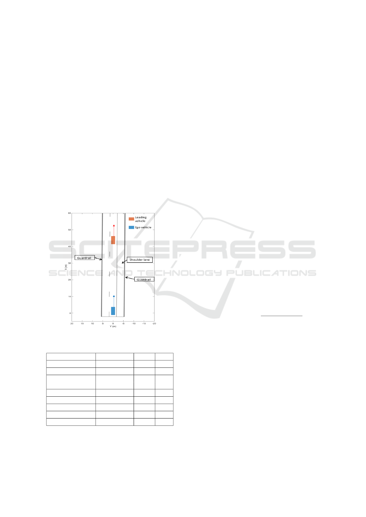
The use case in this analysis has therefore been

based on the likely use case of the chauffeur system

for highways, where an ego-vehicle follows a lead ve-

hicle on a highway. A radar sensor has been mounted

on the ego-vehicle to perceive targets in the environ-

ment. Moreover, the effect of multipath propagation

has been taken into account in the simulation to eval-

uate the radar sensor’s ability to perceive the envi-

ronment. The use case is depicted in the Figure 1

where, the radar has been mounted at the front the

ego-vehicle (blue color) and the guardrail (bold black

color) and the leading vehicle (orange color).

Figure 1: Use case concrete scenario modeling.

Table 1: Scenario modeling parameters.

Object Measure Value Unit

Ego-vehicle Velocity 27 m/s

Lead Vehicle Velocity 27 m/s

Distance Distance 40 m

between vehicles

Simulation Duration 4 s

Simulation Sample time 0.1 s

Driving lane Width 3.75 m

Shoulder lane Width 3 m

Guardrail Height 0.75 m

The relevant parameters of the scenario are shown

in Table 1. The ego-vehicle equipped with a radar

sensor closely tracks the leading vehicle at the same

speed in meter per second (m/s). The duration of the

whole scenario is 4 seconds (s) and the sampling time

is 0.1 s. The width of the lane and shoulder are chosen

to represent a typical highway. The values used to

set up the highway have been taken from road and

transportation research association, Germany (FGSV,

2011).

3.3 Sensor Models

A statistical radar model and a physical radar model

have been examined to evaluate sensor performance,

and an use case scenario has been simulated. The

radar effect (multipath propagation) has been evalu-

ated with both sensor models to determine the poten-

tial functional insufﬁciency. As a by-product, poten-

tially safety-critical triggering conditions have been

achieved with respect to SOTIF and support FuSa as

well for a HAD system.

The statistical radar sensor model provided by

MATLAB corresponds to the medium-ﬁdelity sensor

models (Schlager et al., 2020). The statistical radar

sensor model requires lower computational time than

higher ﬁdelity sensor models. The use of statistical

radar sensor models make sense in the early begin-

ning of the developing process, where ﬁrst ideas and

design trade-offs are being investigated. Due to the

relatively low computational time, it is recommended

to use this model also for longer simulations, but

also test tracking and sensor fusion algorithms (Math-

works, 2022b). The sensor model does not consider

signal processing and is only the fundamental for the

principles of automotive radar expressed as (Math-

works, 2022f):

Received power, P

∗ G

∗ σ

(4π)

∗ R

∗ L

(1)

Where, G

deﬁnes the gain of the transmitter. G

indi-

cates gain of the receiver. λ is the wavelength of the

radar’s operating frequency in meters (m). σ specify

the radar cross section of the target in square meters

) R display the range between radar sensor and tar-

get in meter (m). L shows the loss factor according to

the transmitter and receiver and the propagation loss.

In radar range measurement, the maximum dis-

tance between the transceiver and the target depends

on the received power P

. Typically, the radar mea-

surement contains noise, so the target can only be de-

termined if the power at the receiver reaches a mini-

mum power P

rmin

. The minimum power P

rmin

has to

achieve a sufﬁcient SNR to be distinguishable from

the noise of the radar measurement. The resulting

equation for the maximum range is as follows (Wolf,

2022):

A Simulation-Based Testing to Evaluate and Improve a Radar Sensor Performance in a Use Case of Highly Automated Driving Systems

Maximumrange, R

max

∗ G

∗ λ

∗ σ

min

∗ (4π)

∗ L

(2)

Since the radar sensor uses electromagnetic waves

that are traveling between the transceiver and the tar-

get, the time-of-ﬂight (∆t) of the signal can be mea-

sured. Relating to the speed of light c and the men-

tioned ∆t the distance R can be determined as follows

(Herz, 2017):

Distance, R =

∆t ∗ c

(3)

The velocity on the other hand is determined by the

Doppler effect as expressed in (Herz, 2017):

Doppler f requency, f

= f

− f

2 ∗ f

∗ v

(4)

The Doppler frequency F

can be determined by the

difference between the frequency of the transmitted

signal f

and the received signal f

or with the corre-

sponding radial velocity of the target v

in m/s as unit.

The I/Q stands for ”In-phase” and ”Quadrature”. I/Q

signals consist of two sinusoidal, which have identi-

cal frequencies but are 90° out of phase. I/Q signals

are amplitude modulated and the amplitude of the re-

sulting signal can be determined as follows (Podcast,

2022):

Amplitude, A =

+ Q

(5)

Here, I and Q results regarding to the angular depen-

dencies as I = A * cosθ and Q = A * sinθ. The phase

of the signal is (Podcast, 2022),

Phase, θ = tan

−1

(6)

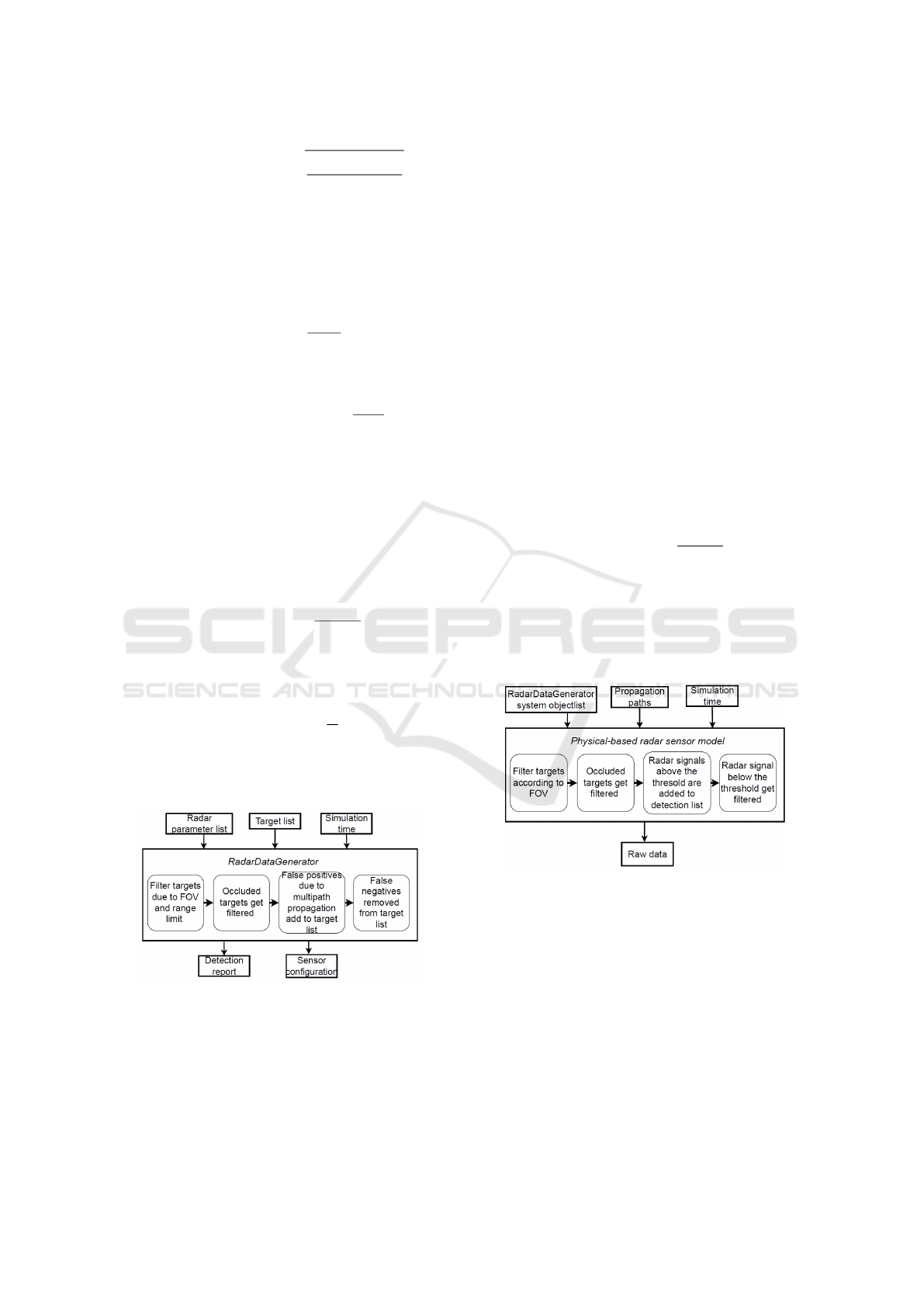
The structure of the statistical sensor model based

on the scheme of medium-ﬁdelity has been presented

in Figure 2.

Figure 2: Block diagram of statistical radar model.

Figure 2 has the top three blocks showing the in-

puts required to create the radar sensor model. The

middle block RadarDataGenerator containing four

steps that the sensor model performs to process the

input data. The bottom portion of Figure 2 represents

the outputs provided by the radar sensor model.

The physics-based radar sensor model has also

been observed to correspond to medium accuracy sen-

sor models, such as the radar sensor model presented

for statistical radar model. The difference between

the statistical radar sensor model and the physics-

based radar model is that the latter generates sam-

pled I/Q signals. These I/Q signals are converted

into target detection. In a addition, the physics-based

model also takes into account the transmitted wave-

form, the propagation of the signal in the simulated

environment, reﬂections from the targets, and signals

received at the receiving facility.

The waveform of the modeled radar transceiver is

a pulse Doppler radar waveform. To set the wave-

form, the Pulse Repetition Frequency (PRF), which

is calculated from the Doppler resolution ∆ f in this

sensor model, and the number of pulses (N) has to

be determined as follows (Gamba, 2020; Mathworks,

2022i):

Pulserepetition f requency, PRF = ∆ f ∗ N

(7)

Magnitude, N

∆ f ∗ T

(8)

The magnitude N

, represents the number of pulses,

which are sent out per one measurement and is calcu-

lated as follows, where ∆f is Doppler resolution and

the pulse width.

Figure 3 depicts the structure of the physics-based

radar model.

Figure 3: Block diagram of physical-based radar model.

The physics-based radar sensor model uses MAT-

LAB’s system object radarTransceiver to generate

I/Q signals in the time domain (Mathworks, 2022i).

This virtual radar transceiver can be generated by the

equivalent radarDataGenerator, that is also needed

to create the statistical radar sensor model. Conse-

quently, it is a part of the input for the physically

based radar sensor model. The propagation paths

have been computed in an auxiliary function provided

by MATLAB. The output of this function provides in-

formation in a detailed structure of every propagation

path. The path of the signal is measured starting at the

SENSORNETS 2023 - 12th International Conference on Sensor Networks

transmitter and ending at the receiver. The path loss L

in decibel of the waveform λ which propagates over

the distance R in meters (m) (Mathworks, 2022c)

Pathloss, L = 20log

(

4πR

) (9)

The reﬂection coefﬁcient describes a speciﬁc magni-

tude of the propagation path depending on how many

times the signal bounces off a reﬂective surface. RCS

deﬁnes the reﬂection coefﬁcient surface. If the signal

bounces off a surface once or twice, the reﬂection co-

efﬁcient becomes smaller. It is calculated as follows,

with the corresponding radar cross section of the tar-

get and the wavelength (Mathworks, 2022a).

Re f lectioncoe f f icient, Re f

co f f

4π

∗ RCS (10)

Finally, the last ﬁeld of the structure contains the

Doppler shift of the received signal, which is calcu-

lated by the radial velocity (v

) of the target, given

in meters per second and the wavelength λ. The re-

sulting Doppler frequency ∆f is given in hertz (Math-

works, 2022h).

Doppler f requency, ∆ f =

(11)

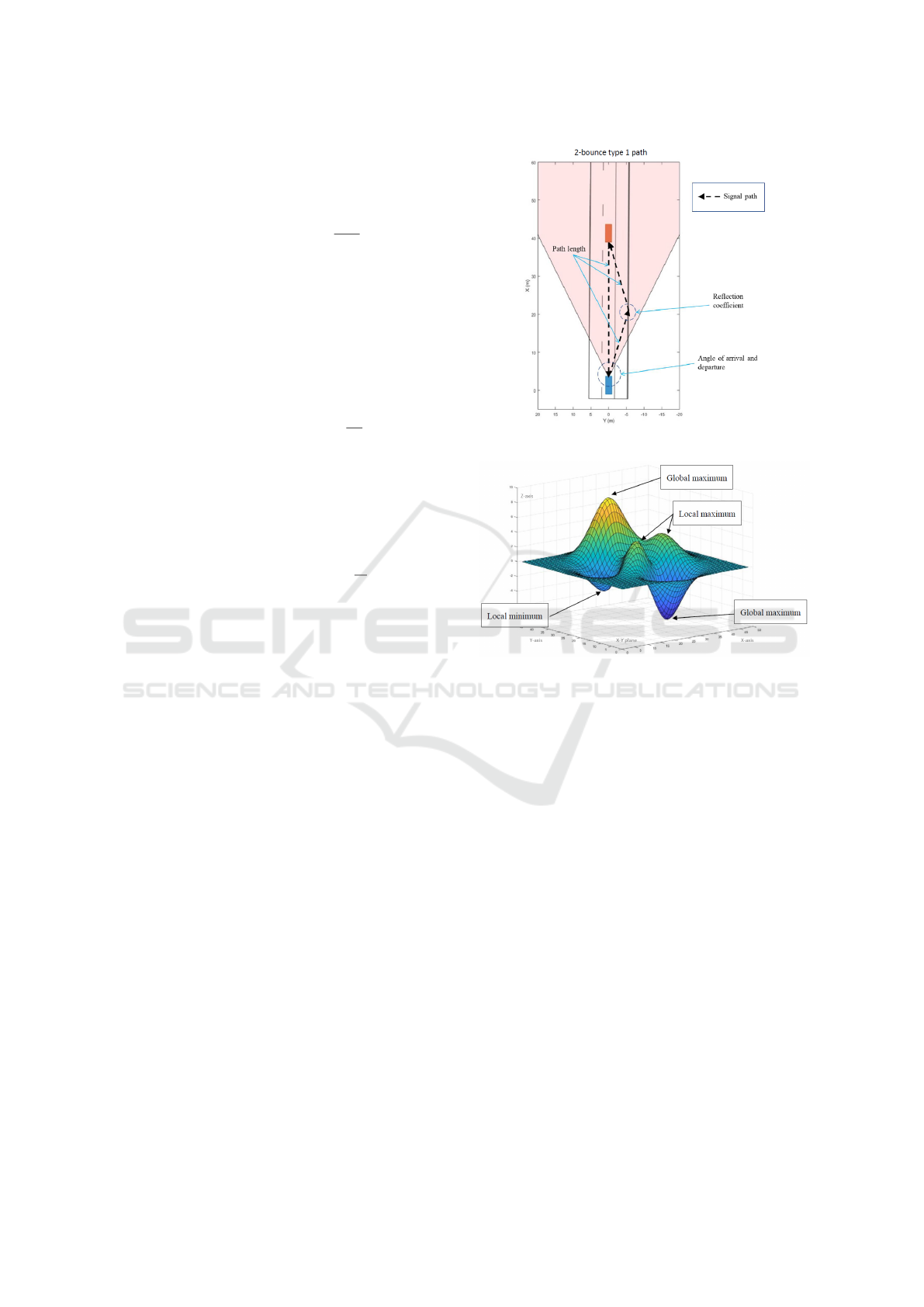
The physics-based radar sensor model has used

all propagation paths as shown in Figure 4, as input

for the radarTransceiver system object. The result-

ing output consists of the corresponding sampled I/Q

signals based on the related signal processing settings

and calculations.

Figure 5 has represented a two-dimensional data

set with local and global maxima and local and

global minima from three-dimensional surface plot

(x-y plane is deﬁned by X and Y and Z as surface

height) (Liske, 2022). For example, the local maxima

has indicated by the values at the highest point of a

curve within a certain range. The highest and lowest

values of the entire data set has been manifested by

the global maximum and global minimum.

The resulting local maxima inclusively the global

maximum represents the SNR of the potential targets.

With the location of each local maxima in the data

set, the relative position of the target can be deter-

mined. This has been accomplished with the result-

ing location of the SNR in the corresponding fast-

time domain. Since the fast-time samples represents

the range bins, the determined location of the local

maxima in the fast-time domain is used to identify the

range. The determination of local maxima is also used

for identifying the azimuth angle of the targets. Due

to the phase shift beam-forming, each scanning angle

can be considered. Therefore, the position of the lo-

cal maxima in the second dimension of the radar data

Figure 4: Propagation path of 2-bounce type 1 properties.

Figure 5: Representation of global and local max-

ima/minima in a 2D data set (Liske, 2022).

cube indicates the corresponding angle where the tar-

get is located (Mathworks, 2022e). The local maxima

has been presented in both sensor models as simula-

tion outcomes.

4 SIMULATION-BASED TESTING

IMPLEMENTATION

4.1 Implementation

The radar-related visualization in this study consists

of the Field Of View (FOV) and radar detection rep-

resented as colored dots. Black colored dots are true

positive detection, meaning they represent detection

that have the associated signal transmitted directly be-

tween the radar and the target. The orange and red

dots indicate which propagation path the detection is

based on, as displayed in Figure 6.

The structure of the implementation process for

the statistical radar sensor model in MATLAB is

demonstrated in Figure 6. MATLAB provides an

A Simulation-Based Testing to Evaluate and Improve a Radar Sensor Performance in a Use Case of Highly Automated Driving Systems

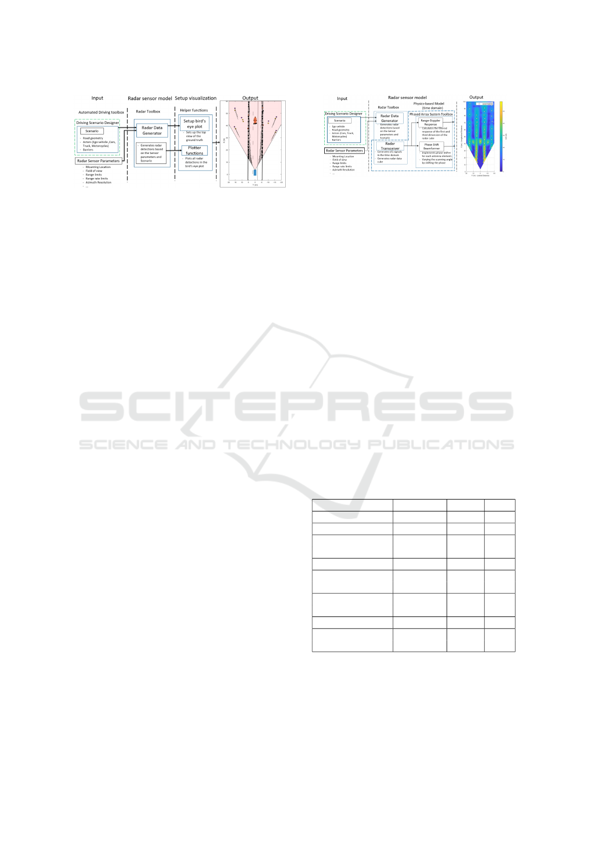
Figure 6: Implementation of statistical radar sensor model.

application, which is called “Driving Scenario De-

signer” (Mathworks, 2022g; Mathworks, 2022d).

This application has been included from the auto-

mated driving toolbox and provides a graphical in-

terface to build a scenario. The modeled scenario

has been exported as a MATLAB function and im-

plemented in the radar sensor model with the help of

Equations (1)-(6). The Radar data generator, a sys-

tem object provided by the radar toolbox generates

the detection. These detection are based on the de-

ﬁned radar sensor parameters and the scenario param-

eters. The output of the Radar data generator is used

by so-called “helper functions” to output the visual-

ization of the scenario with the corresponding radar

detection (Mathworks, 2022g).

The physics-based radar sensor model can be seen

as the extension of the statistical radar sensor model.

A radar transceiver is modeled to generate I/Q signals

in the time domain that are represented the returning

signals. These returning signals are generated based

on the possible propagation paths which results be-

tween the environment and the radar.

In Figure 7 the radartransceiver system object

is included in the MATLAB’s radar toolbox (Math-

works, 2022b). To process the resulting radar data

cube, which contains the sampled I/Q signals, the

MATLAB’s phased array system toolbox is consid-

ered. This toolbox includes radarDopplerResponse

system object and the phaseShiftBeamformer system

object. The former one is used to process the range

by Equation (2) and Doppler information by Equation

(11), that is included in the radar data cube and the lat-

ter one is used to vary the scanning angle to extract the

angle information out of the data cube (Mathworks,

2022e).

Further, the resulting raw data can be used to visu-

alize the distribution of the SNR in the measurement

in an appropriate range-angle map, which is also rep-

resented in Figure 7.

4.2 Radar Sensor Setup and Simulation

The ego-vehicle in the use case scenario has been

equipped with a forward-facing mono-static radar.

Figure 7: Implementation of physical-based radar sensor

model.

The sensor’s transmitter and receiver are therefore lo-

cated in one place. Currently, the radar sensors used

to implement advanced driver assistance systems and

automated driving functions operate at a frequency of

76 GHz to 77 GHz (Mathworks, 2022f). The radar

sensor is located 0.2 m above the ground in the center

of the front bumper of the ego-vehicle. According to

(Ziegler et al., 2014), the FOV of the radar and the

maximum detection range are based on the setup for

the long-range radar used for the Bertha Benz test ve-

hicle. The azimuth angle resolution for conventional

radar sensors is given between 1.5° and 4° according

to (Yu et al., 2022). In the radar sensor setup pre-

sented in this paper, the azimuth angle is set to 2°

to achieve a higher resolution in the angle measure-

ment. The range resolution is set to 2.5 m and thus to

a smaller size corresponding to the length of a vehicle.

Finally, the limits of the range rate are set to the range

corresponding to the maximum allowable operating

speed of the driving function of 100 m/s. The radar

sensor has the ability to detect the varying speeds of

the targets in steps of 0.5 m/s within the distance lim-

its as listed in Table 2.

Table 2: Radar model parameters.

Object Measure Value Unit

Center frequency Frequency 77 GHz

Sensor Mounting Height 0.2 m

FOV Azimuth/ 56/9 deg

Elevation

Maximal Range Distance 60 m

Range rate Velocity -100... m/s

limits Elevation 100

Angle Azimuth 2 deg

resolution angle

Range resolution Distance 2.5 m

Range rate Velocity 0.5 m

resolution

The statistical radar sensor model has been ap-

plied to simulate the scenario described in section 3.

A snapshot of a scene from the scenario is viewed in

Figure 8. This snapshot shows the overhead view of

the scene, also referred to as a bird’s eye view. Fig-

SENSORNETS 2023 - 12th International Conference on Sensor Networks

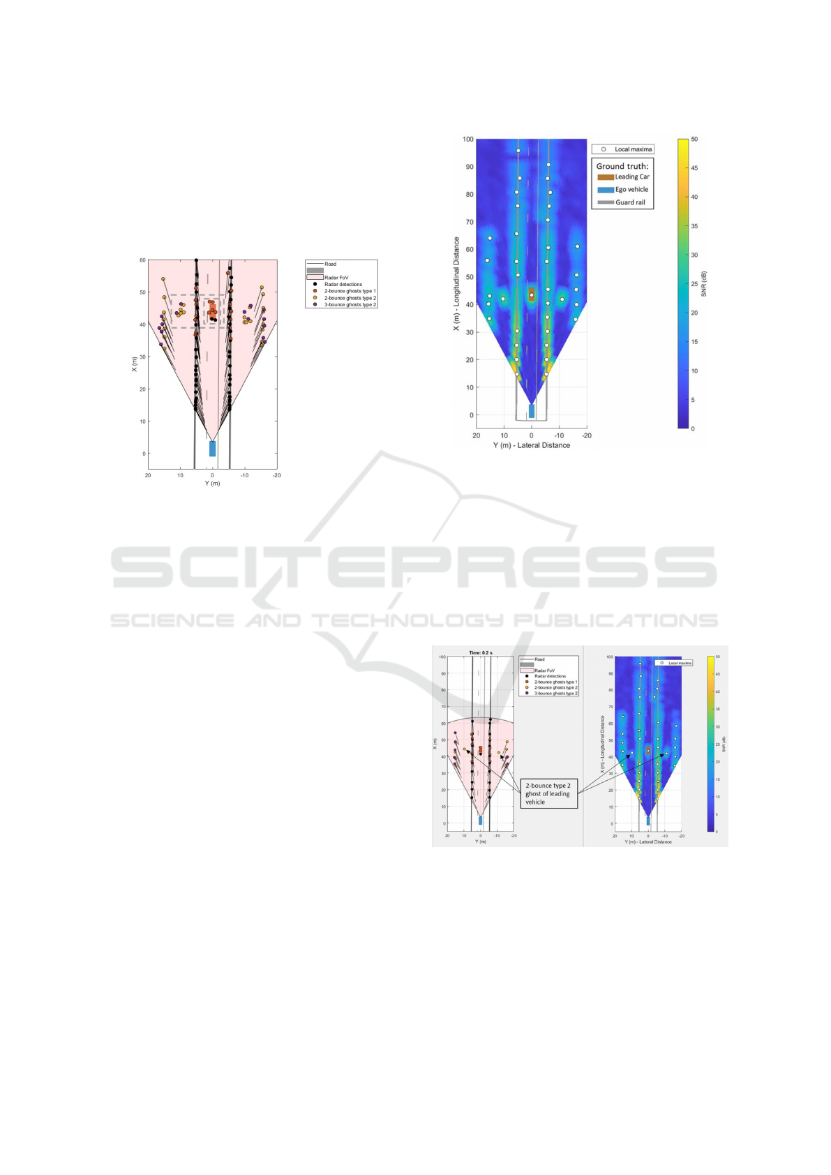
ure 8 has primarily shown the ground truth data of

the environment, which includes the road, guardrails,

and the two vehicles (ego-vehicle: blue and leading

vehicle: orange). The radar sensor’s coverage area,

which is the area deﬁned by the speciﬁc FOV, and the

maximum coverage area are also illustrated in Figure

Figure 8: Top view of the scene (statistical radar sensor

model).

The statistical radar sensor model generates a re-

port that contains information about the relative posi-

tion of each detection. Depending on the position, the

detection points are plotted as dots in the bird’s eye

view, as shown in Figure 8. Within the radar sensor’s

detection area, the radar detection points are shown as

black and colored dots as visible in Figure 8.

The physics-based sensor model includes the

radar-speciﬁc waveforms in the time domain and the

corresponding signal processing part. Since the re-

sulting output of this type of sensor model consists

of raw data, the information has to be interpreted

differently than for example the statistical radar sen-

sor model. This radar-speciﬁc raw data has included

range, angle, and Doppler information. To represent

the position of targets in a bird’s eye view, the pro-

cessed range and angle information has been used

to create the visualization. The architecture of the

physics-based sensor model was described in the pre-

vious section 3.

The Figure 9 provides a bird’s eye view of the

distribution of the SNR with the support of radar re-

ceived power that has been calculated with the support

of Equations (1), (9) and (10), together with the cor-

responding local maxima. Thus, the targets based on

the generated I/Q signals and the corresponding sig-

nal processing can be performed. The ground truth

data has been presented by Figure 9 for a speciﬁc use

case scenario.

Figure 9: Top view of the scene (physical-based radar sen-

sor model).

4.3 Results and Discussions

Since the statistical radar sensor model and the

physics-based radar sensor model are subject to dif-

ferent architectures, the output measurement varies in

some respects as marked in Figure 10. Both sides of

the Figure 10 reveal a snapshot of the scenario at time

0.2 s.

Figure 10: Snapshot of both radar sensor models.

The maximum unique detection range has been

observed in Figure 10 for both sensor models. In one

hand, the statistical radar sensor model sets its detec-

tion range only to the maximum range value as de-

ﬁned in Table 2. On the other hand, physics-based

radar sensor model has wide range. the maximum

range is determined by the PRF. The PRF is calcu-

lated through Equation (7) and Equation (8). The PRF

A Simulation-Based Testing to Evaluate and Improve a Radar Sensor Performance in a Use Case of Highly Automated Driving Systems

depends on the number of pulses that are sent out per

measurement and the range rate resolution, which is

also deﬁned in Table 2.

Table 3: Relative position and SNR for statistical radar

model.

Properties ∆x ∆y SNR

Ground truth 42.41 m -0.05 m -

Desired 41.38 m -0.03 m 20.67 dB

detection

2-bounce 45.42 m 0.07 m 17.35 dB

type 1 ghost

2-bounce type 44.45 m 9.76 m 19 dB

2 ghost left

2-bounce type 42.34 m -10.92 m 18.81 dB

2 ghost right

Table 3 illustrates the measurement data of desired

detection, ghost detection due to multipath propaga-

tion, and ground truth data of the leading vehicle. The

ground truth is presented as the actual relative posi-

tion (∆x, ∆y) and SNR by the measurement data pro-

vided by the simulation as recorded in Table 3. For

example, The SNR rate of the desired detection has

been achieved by statistic radar model is ≈ 20 dB.

The values of the measurement according to the de-

sired detection almost correspond to the ground truth

data. This is an evidence that the black dots represent

adequate detection of the target by the radar. The red

dots are 2-bounce type 1 ghost images, meaning that

the radar signal bounces off a reﬂective surface on its

way to the target. Reﬂection off a surface results in

a longer time of ﬂight for the radar signal and thus a

greater relative distance.

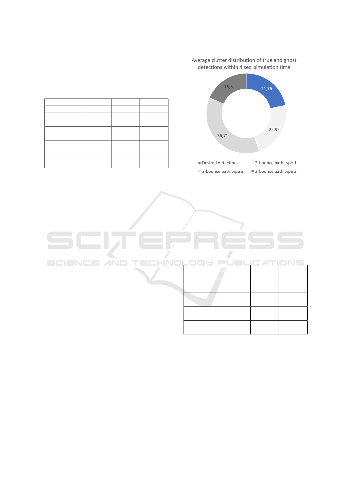
An illustration of a pie chart in Figure 11 contains

all the dynamic detection within the simulation time

of 4 s. Since the sample time of the simulation is 0.1 s,

the resulting simulation steps equal to 40. Therefore,

in every simulation step, the distribution of desired

detection and ghost detection is evaluated and added

up.

The pie chart in Figure 11 sketches the percentage

distribution of ghost detection. The greatest propor-

tion has been covered by the 2-bounce path type 2

ghosts with ≈36%. The 3-bounce path type 2 ghost

has the lowest proportion with about half of the 2-

bounce ghosts with ≈18%. The area has been cov-

ered by 2-bounce type 1 ghosts and desired detection

is ≈21% and ≈22%. respectively. According to this

analysis, the amount of ghost/false detection is rela-

tively high.

The simulation results based on the physical-

based radar has been presented in Table 4 with respect

to the outcomes as relative position (∆x, ∆y) and SNR.

Figure 11: Percentage distribution of detection for statisti-

cal radar sensor model.

The desired detection rate has SNR value of ≈25dB

for physical-based radar model. Table 3 and Table

4 have represented the relative position and the SNR

of the desired detection and the ghost detection of the

leading vehicle considering the outcomes of statistical

radar model and physical-based radar model accord-

ingly.

Table 4: Relative position and SNR for physical-based radar

model.

Properties ∆x ∆y SNR

Ground truth 42.41 m -0.05 m -

Desired 41.40 m 0 m 25.02 dB

detection

2-bounce - - -

type 1 ghost

2-bounce type 42.21 m 9.68 m 17.66 dB

2 ghost left

2-bounce type 41.85 m -10.02 m 24.01 dB

2 ghost right

In this simulation the position of the radar detec-

tions is compared with the ground truth. Addition-

ally, If a local maxima does not cover an object’s

ground truth, it will be considered as ghost target.

According to the simulation results from physical-

based radar sensor model, true detection is performed

≈49% and able to detect the leading vehicle approxi-

mately ≈94% as exhibited in Figure 12.

The results have been represented on the basis of a

”true” or ”false” detection. This is done by checking

whether a local maximum covers an object of ground

truth. If this is the case, it can be assumed that the

radar is detecting the object correctly, and the detec-

SENSORNETS 2023 - 12th International Conference on Sensor Networks

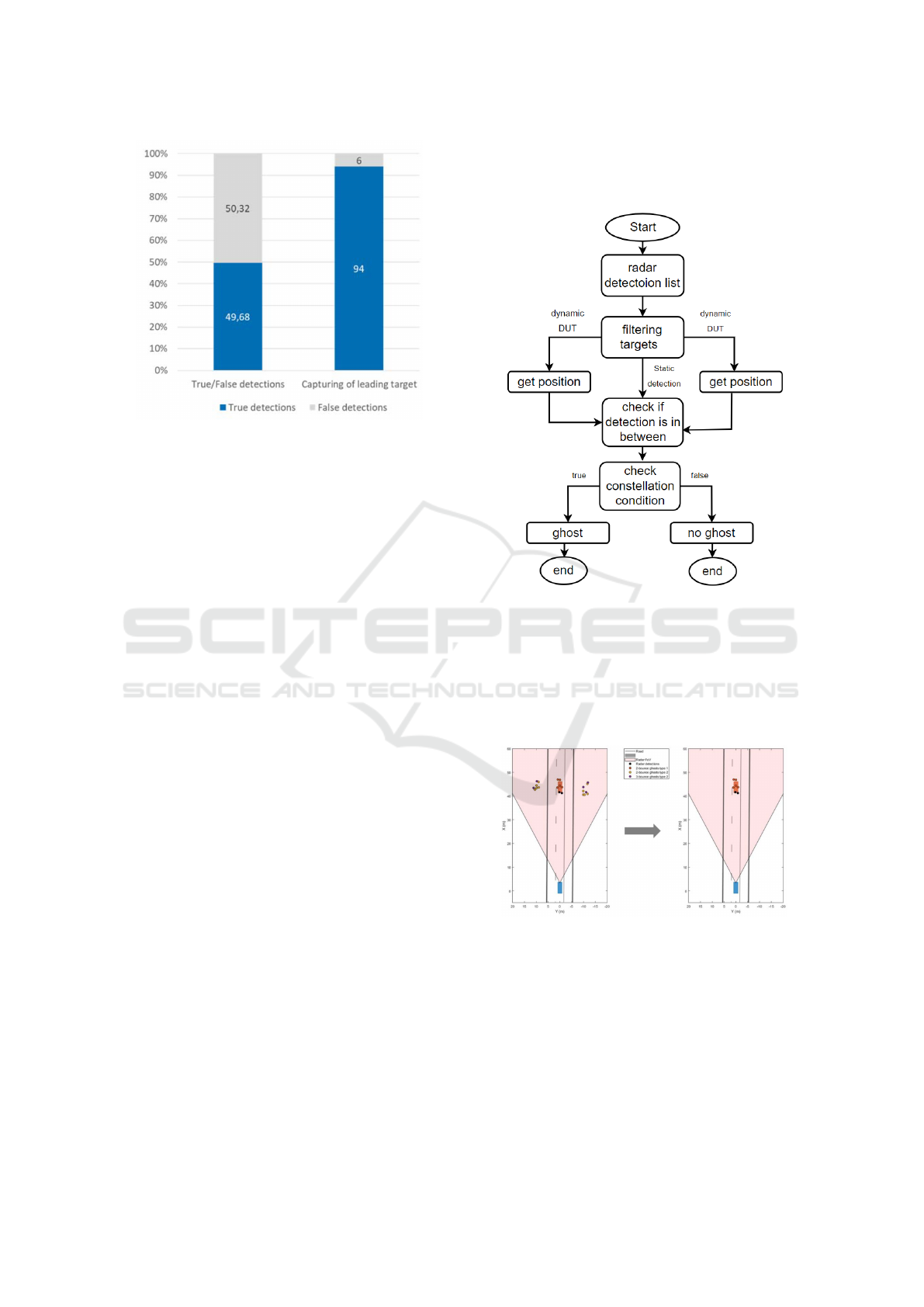
Figure 12: Detection of leading vehicle by physical-based

radar sensor model.

tion in this case is called a ”correct detection”. All

other detections that do not cover a ground truth ob-

ject are referred to as ”false detection”.

Furthermore, the simulation results validate the

detection of the leading vehicle by the radar sensor

throughout the simulation. Since the methods de-

scribed in the previous subsection consider the ground

truth object covered by a local maximum, it is possi-

ble to check whether the radar sensor detects the lead-

ing vehicle during the entire simulation.

4.4 Sensor Performance Improvement

From the simulation results of the statistical radar sen-

sor model, the highest proportion of ghost targets are

the 2-bounce type 2 ghosts. The analysis of the SNR

of the physics-based radar sensor model has shown

that such ghost detection can have characteristics like

real detection. Moreover, the physics-based radar sen-

sor model has yielded as a result that the leading vehi-

cle is captured most of the simulation time. Accord-

ing to these results, a ﬁlter development has great em-

phasis that can identify 2-bounce and 3-bounce type

2 ghosts. Hence, a ﬁlter has been modeled and tested

for the use case.

The developed ﬁlter has focused only on detec-

tion after moving objects. Since the radar sensor in

the physics-based model almost always detects the

leading vehicle, the 2-bounce type 1 ghosts are dis-

regarded in this case. For Type 2 ghost have been

located outside the road. Because the angle of the

returning signal results from the signal bouncing off

the guardrail as it returns to the sensor after reﬂect-

ing off the vehicle ahead, these type 2 ghost images

are projected onto the other side of the guardrail. The

concept ﬂow diagram of the developed ﬁlter has been

laid-out in Figure 13. The following ﬂow diagram in

Figure 13 has conveyed the rough structure of the al-

gorithm.

Figure 13: Flow diagram of the ﬁlter algorithm.

A reduced amount of type 2 ghosts points has

been the after-effect of the developed ﬁlter for statistic

radar model and appeared in the Figure 14. The left

and right sides of Figure 14 have detection points with

type 2 ghost points and the corresponding ﬁltered type

2 ghost points.

Figure 14: Radar detection without ﬁlter (left). Radar de-

tection with ﬁlter (right).

Due to the fact that the detection list of the statis-

tical radar sensor model contains detailed data about

each detection, only the speciﬁc raw data such as rel-

ative velocity and relative position have been used to

implement the ﬁlter. Thus, it will be possible to ap-

ply this ﬁlter to the physics-based radar sensor model

as well. The ﬁrst step, as shown in Figure 13, is to

ﬁlter the static objects in the radar detection list. The

A Simulation-Based Testing to Evaluate and Improve a Radar Sensor Performance in a Use Case of Highly Automated Driving Systems

next step is to select a dynamic detection, called a De-

tection Under Test (DUT). This DUT has been tested

next to determine if it is a type 2 ghost. Another dy-

namic detection has to be selected from the detection

list, which can also be referred to as Detection Un-

der Comparison (DUC). Next, a check has been made

to verify whether there is a static detection between

the DUT and the DUC. If this is the case, it has been

indicated that there is a guard rail between the two de-

tections, indicating that the DUT under consideration

is a Type 2 ghost.

5 CONCLUSION

In this paper, a comprehensive methodology for

simulation-based testing of an automotive radar for a

speciﬁc SOTIF use case scenario has been presented

in a systematic manner. This study has provided a

simulation-based test concept to identify the perfor-

mance insufﬁciency of radar models with respect to

a use case applicable in HAD systems like highway

chauffeur. For simulating the deﬁned use case sce-

nario two kinds of radar models are applied.

Moreover, multipath propagation effect for a radar

sensor has been evaluated by examining both statis-

tical and physical-based radar models. Therefore,

possible triggering conditions has been realized to

support the SOTIF of HAD systems. The statistical

radar model has been used to analyse the occurrence

of ghost targets due to the multipath propagation ef-

fect which leads to an inaccurate perception of the

radar sensor. The simulation results of the statisti-

cal radar sensor model have illustrate that over 75%

of the detection representing the leading vehicle are

ghost detection and thus false positives. The major-

ity of ghosts are 2-bounce type 2 ghosts. Addition-

ally, physics-based radar sensor model has generated

time-domain I/Q signals with signal processing like

range Doppler processing and phase shift beamform-

ing. Therefore, physics-based radar sensor model has

more detailed representation of radar sensors and has

been used to validate the simulation outcomes of the

statistical radar sensor model.

Furthermore, a ﬁlter has been developed to reduce

the type 2 ghost detection as a remedy of functional

insufﬁciency of a radar model in the focus of the re-

ﬂection on guardrails. The improved detection of the

radar with the ﬁler has been presented as an upshots

of this study.

The focus of future work can be to implement

the physics-based radar sensor model in a more com-

plex environment where more environmental inﬂu-

ences and reﬂective surfaces are present. In addi-

tion, the presented simulation-based testing approach

can be used to investigate more use cases considering

multipath propagation to support the veriﬁcation and

validation of a radar sensor.

REFERENCES

Becker, C. J., Brewer, J. C., and Yount, L. J. (2020). Safety

of the intended functionality of lane-centering and

lane-changing maneuvers of a generic level 3 highway

chauffeur system.

Berk, M.and Schubert, O., Kroll, H.-M., Buschardt, B.,

and Straub, D. (2020). Assessing the safety of envi-

ronment perception in automated driving vehicles. 8

(1):49–74.

FGSV (2011). Guidelines for the design of motorways

(raa). https://www.fgsv-verlag.de/pub/media/pdf

/202 E PDF.v.pdf.

Gamba, J. (2020). Radar Signal Processing for Autonomous

Driving. Springer Singapore, Singapore, 1st edition.

Herz, G. (2017). Development of a radar sensor behav-

ior model for validation of advanced driver assistance

systems.

Herz, G., Schick, B., Hettel, R., and Meinel, H. (2019). So-

phisticated sensor model framework providing realis-

tic radar sensor behavior in virtual environments.

IEC/TR63069 (2019). Industrial-process measurement,

control, and automation - framework for functional

safety and security. https://webstore.iec.ch/public

ation/31421.

ISO21448 (2022). Road vehicles — safety of the intended

functionality. https://www.iso.org/standard/77490.h

tml.

ISO26262 (2018). Road vehicle — functional safety, part 1

to part 13. https://www.iso.org/standard/43464.html.

Khatun, M., Caldeira, G., Jung, R., and Glaß, M. (2021a).

An optimization and validation method to detect the

collision scenarios and identifying the safety speciﬁ-

cation of highly automated driving vehicle. In 21st

International Conference on Control, Automation and

Systems (ICCAS), pages 1570–1575.

Khatun, M., Caldeira, G., Jung, R., and Glaß, M. (2021b). A

systematic approach of reduced scenario-based safety

analysis for highly automated driving function. In 7th

International Conference on Vehicle Technology and

Intelligent Transport Systems. Scitepress.

Khatun, M., Glaß, M., and Jung, R. (2020). Scenario-based

extended hara incorporating functional safety and so-

tif for autonomous driving. 30th European Safety and

Reliability Conference.

Leither, A., Watzenig, D., and Ibanez, J. (2020). Valida-

tion and Veriﬁcation of Automated Systems. Springer

Nature Switzerland AG., European Union, 1st edition.

Liske, M. (2022). Master thesis: Simulation-based testing

to improve the sensor limitations for a sotif use case

scenario. In Masther Thesis. Institute for Advanced

Driver Assistance Systems and Connected Mobility-

Kempten University of Applied Sciences.

SENSORNETS 2023 - 12th International Conference on Sensor Networks

Martin, H., Winkler, B., Grubm

uller, S., and Watzenig, D.

(2019). Identiﬁcation of performance limitations of

sensing technologies for automated driving. In 2019

IEEE International Conference on Connected Vehi-

cles and Expo (ICCVE), pages 1–6.

Mathworks (2022a). aperture2gain: Convert effective aper-

ture to gain. https://de.mathworks.com/help/phased/r

ef/aperture2gain.html?searchHighlight=%20ap.

Mathworks (2022b). Create physics-based radar model

from statistical model. https://de.mathworks.com

/help/radar/ug/radar-model-abstract-level.html.

Mathworks (2022c). fspl: Free space path loss. https://de.m

athworks.com/help/phased/ref/fspl.html#:

∼

:text=Des

cription, -example&text=L%20%3D%20fspl(%20R

%20%2C%20lambda%20)%20returns%20th.

Mathworks (2022d). Introduction to statistical radar models

for object tracking. https://www.mathworks.com/help

/fusion/ug/introduction-to-radar-for-object-tracking

.html.

Mathworks (2022e). Radar data cube concept. https://de.m

athworks.com/help/phased/gs/radar-data-cube.html?s

earchHighlight=RADAR%20data%20cube&s tid=s

rchtitle RADAR%252.

Mathworks (2022f). Radar equation: Radar equation the-

ory. https://de.mathworks.com/help/radar/ug/radar-e

quation.html.

Mathworks (2022g). radardatagenerator: Generate radar

detections and tracks. https://de.mathworks.com/h

elp/radar/ref/radardatagenerator-system-object.html.

Mathworks (2022h). speed2dop: Convert speed to doppler

shift. https://de.mathworks.com/help/phased/ref/spe

ed2dop.html?searchHighlight=speed2do.

Mathworks (2022i). time2range: Convert propagation time

to propagation distance. https://de.mathworks.com/h

elp/phased/ref/time2range.html?searchHighlight=tim

e%25.

Mazzega, J. (2019). Pegasus method: An overview. PE-

GASDU Symphony.

Parker, M. (2017). Chapter 20-automotive radar with contri-

butions by ben esposito. In Parker, M., editor, Digital

Signal Processing 101 (Second Edition), pages 253–

276. Newnes, 2nd edition.

Podcast (2022). Understanding i/q signals and quadrature

modulation: Chapter 5 - radio frequency demodula-

tion. https://www.allaboutcircuits.com/textbook/radi

o-frequency-analysis-design/radio-frequency-demo

dulation/understanding-i-q-signals-and-quadrature-

modulation/.

SAEJ3016 (2021). Taxonomy and deﬁnitions for terms re-

lated to driving automation systems for on-road motor

vehicles. https://www.sae.org/standards/content/j301

6 202104/.

Schlager, B., Muckenhuber, S., Schmidt, S.and Holzer, H.,

Rott, R.and Maier, F. M., Saad, K., Kirchengast, M.,

Stettinger, G., Watzenig, D., and Ruebsam, J. (2020).

State-of-the-art sensor models for virtual testing of ad-

vanced driver assistance systems / autonomous driv-

ing functions. SAE International Journal of Con-

nected and Automated Vehicles, 3(3):233–261.

UL4600 (2022). Standard for evaluation of autonomous

products. https://ul.org/UL4600.

Valdez Banda, O. A. and Goerlandt, F. (2018). A stamp-

based approach for designing maritime safety man-

agement systems. Safety Science, 109:109–129.

Winner, H., Hakuli, S., Lotz, F., and Singer, C.

(2015). Handbuch Fahrerassistenzsysteme: Grund-

lagen, Komponenten und Systeme f

ur aktive Sicher-

heit und Komfort. Springer Vieweg Wiesbaden, Wies-

baden, 3rd edition.

Wolf, C. (2022). The radar range equation, argumenta-

tion/derivation. https://www.radartutorial.eu/01.ba

sics/The%20Radar%20Rang%20Equation.en.html.

Yu, W., Li, J., Peng, L.-M.and Xiong, X., Yang, K., and

Wang, H. (2022). Sotif risk mitigation based on uni-

ﬁed odd monitoring for autonomous vehicles. Journal

of Intelligent and Connected Vehicles.

Zhou, Y., Liu, L., Zhao, H., L

opez-Ben

ıtez, M., Yu, L., and

Yue, Y. (2022). Towards deep radar perception for au-

tonomous driving: Datasets, methods, and challenges.

Sensors, 22(11).

Ziegler, J., Bender, P., Schreiber, M., Lategahn, H., Strauss,

T., Stiller, C., Dang, T., Franke, U., Appenrodt, N.,

Keller, C. G., Kaus, E., Herrtwich, R. G., Rabe, C.,

Pfeiffer, D., Lindner, F., Stein, F., Erbs, F., Enzweiler,

M., Kn

oppel, C., Hipp, J., Haueis, M., Trepte, M.,

Brenk, C., Tamke, A., Ghanaat, M., Braun, M., Joos,

A., Fritz, H., Mock, H., Hein, M., and Zeeb, E. (2014).

Making bertha drive—an autonomous journey on a

historic route. IEEE Intelligent Transportation Sys-

tems Magazine, 6(2):8–20.

A Simulation-Based Testing to Evaluate and Improve a Radar Sensor Performance in a Use Case of Highly Automated Driving Systems