Task Scheduling: A Reinforcement Learning Based Approach
Ciprian Paduraru, Catalina Camelia Patilea and Stefan Iordache
Faculty of Mathematics and Computer Science, Department of Computer Science,
University of Bucharest, Bucharest, Romania
Keywords:
Job Shop Scheduling, Task Distribution, Reinforcement Learning, DQN, Dueling-DQN, Double-DQN, Policy
Optimization, Supervised Task Scheduling, Genetic Algorithms.
Abstract:
Nowadays, various types of digital systems such as distributed systems, cloud infrastructures, industrial de-
vices and factories, and even public institutions need a scheduling engine capable of managing all kinds of
tasks and jobs. As the global resource demand is unprecedented, we can classify task scheduling as a hot topic
in today’s world. On a small scale, this process can be orchestrated by humans without the intervention of
machines and algorithms. However, with large scale data streams, the scheduling process can easily exceed
human capacity. An automated agent or robot capable of processing millions of requests per second is the ideal
solution for efficient scheduling of flows. This work focuses on developing an agent that learns autonomously
from experiences using reinforcement learning how to perform efficiently the scheduling process. Carefully
designed environments are used to train the agent to have similar or better planning experiences than already
existing methods such as heuristic algorithms, machine learning-based methods (supervised algorithms) and
genetic algorithms. We also focused on designing a suitable dataset generator for the research community, a
tool that generates random data starting from a user-supplied template in combination with different distribu-
tion strategies.
1 INTRODUCTION
Our main observation in the field of applying method-
ologically task scheduling processes is that extensive
decision making are part of our lives more than ever.
From 2020 to 2021, Uber Eats scaled up and now they
are delivering food in more than 6000 cities world-
wide, up from close to 1000 cities before the COVID-
19 pandemic started (Li et al., 2021). Those num-
bers, along with close to one million restaurants reg-
istered in the application and over 80 millions active
users, placed a huge strain on the computational sys-
tems behind Uber Eats and this is not a singular case.
Multiple industries are dependent on task schedul-
ing systems and algorithms, this mission being also
known as ”Job Shop Scheduling”, a famous NP-hard
(non-deterministic polynomial-time) problem (Letch-
ford and Lodi, 2007).
The work presented in this paper is focused on ex-
ploring current approaches on task scheduling and it
also adds improvements by developing a framework
that can be adapted to different scenarios. The frame-
work developed during this work is called TSRL
(Task Scheduling - Reinforcement Learning) and it
was used by use to train agents used for cloud re-
source scheduling (Asghari et al., 2020) (Song et al.,
2021). Since task scheduling has been heavily used in
the area of distributed systems we’ve considered that
we can add value to this domain by creating a soft-
ware that can be added to cloud environments or even
data centers. This will act as an agent that learns the
resource demand over time and can be later used to as
a control module that regulates how many resources
an application is allowed to use, based on importance
and profit metrics.
Our contributions within this research can be fur-
ther divided into two main components:
• A reusable open-source environment (based on
the OpenAI Gym interface (Brockman et al.,
2016)) designed for multiple workers and re-
source types, and easily adaptable to different
cases of task scheduling problems. Along with
this environment, we add a dataset and methodol-
ogy to collect it synthetically without human ef-
fort.
• A novel reinforcement learning (RL) (Sutton and
Barto, 2018) based algorithm that is comparable
to or outperforms the state of the art on some
metrics and use cases for the resource scheduling
problem.
The work described in this research paper is open-
source, but due to double blind review constraints we
can’t list it.
948
Paduraru, C., Patilea, C. and Iordache, S.
Task Scheduling: A Reinforcement Learning Based Approach.
DOI: 10.5220/0011826100003393
In Proceedings of the 15th International Conference on Agents and Artificial Intelligence (ICAART 2023) - Volume 3, pages 948-955
ISBN: 978-989-758-623-1; ISSN: 2184-433X
Copyright
c
 2023 by SCITEPRESS – Science and Technology Publications, Lda. Under CC license (CC BY-NC-ND 4.0)

From our study we’ve understood that in some
cases severe solutions may be preferred, an agent
that is able to schedule tasks before the deadline,
while other scenarios will focus only on achieving a
larger profit margin where deadlines are less impor-
tant. During our development we’ve focused on the
first part, considering a high degree QoS (Quality of
Service) and obtaining lower number of SLA (Service
Level Agreement) violations as main objectives.
For our packet scheduling scenario, we adapted
from the literature, two main RL algorithms: (a)
State-Action-Reward-State-Action (SARSA) (Rum-
mery and Niranjan, 1994), and (b) Q-Learning (Jang
et al., 2019). Both are iterative algorithms by nature,
since the nonexistence of final states affects the time
required for learning. Our contribution to adapting
them to our method and goals are some changes we
have made to ensure better exploration of states and
actions at the very beginning of each learning session.
Literature also investigated methods such as Deep Q-
Networks (DQN) (Mnih et al., 2013), Deep Determin-
istic Policy Gradients (DDPG) (Silver et al., 2014),
and Actor-Critics (Konda and Tsitsiklis, 2001), which
we also compare in our evaluation section.
The rest of the paper is organized as follows. The
next section presents some theoretical backgrounds in
the area of RL, scheduling algorithms, and sets up the
abstract definition of the problem addressed in this pa-
per. Section 3 describes the method used to put the
scheduling algorithm closer to usage in practice, i.e.,
deployment perspective, and defines our problem as a
Markov chain such that it can be used with RL based
methods.
2 THEORETICAL BACKGROUND
2.1 Task Scheduling
Our objective is to efficiently distribute jobs across
different systems and environments. It may be mis-
leading, but we believe that scheduling is not just
about finding the best algorithm for a very specific
case. Instead, we focus on prototyping a framework
that can be used to replicate user customized busi-
ness scenarios end-to-end, from data generation to
the scheduling agent or algorithm itself. Such sys-
tems should be developed around some key metrics
or standards to be met, for example: resources unifor-
mity, high availability and quality of service parame-
ters (QoS).
2.2 Datasets
In many industries, businesses and research, data us-
age exceeds terabytes and even petabytes. Aggregat-
ing and extracting features from such large collec-
tions is a difficult and costly process. In contrast, it
is almost impossible to develop a digital scheduler for
cases where the data is collected and stored offline.
Considering these facts, we have tried to find a
solution that balances both problems by generating
whole datasets in a parameterized way starting from
a summary data analysis. Each set of values is gener-
ated starting with basic distributions: normal, uniform
or exponential. Furthermore, those distributions can
be combined into more advanced scenarios that sim-
ulate workloads of modern systems (Shyalika et al.,
2020), especially when we talk about digital applica-
tions and computer systems (data centres, clusters):
• Stress Scenarios – this category can be divided
into two parts, spike and soak, the first one de-
scribing a sudden increase in workload and the
second one in large volumes of tasks (constant)
over a long period of time.
• Load Scenarios – a constant flow of tasks is
present in the system (starting with a specific con-
figuration of the environment). We want to obtain
an algorithm that can digest more jobs, over the
current load.
The reward is computed based on the time spent
for the actual computation and how the environment
looked during the execution. Tasks that are finished
over the deadline are awarded with a negative score
and those who are marked as completed earlier do of-
fer a positive reward.
2.3 Reinforcement Learning: Quick
Overview
Essentially, Reinforcement Learning (RL) is a
paradigm that focuses on the development of agents
that can interact with different environments in
stochastic spaces. Clear labelling is not provided, but
the goal is the same: maximizing a reward function
over time. Therefore, we can describe reinforcement
learning as a semi-supervised strategy, a distinct class
of machine learning algorithms. There are several
core components that describe a reinforcement learn-
ing algorithm:
• States (S).
• Actions (A).
• Policy (π) - it defines a particular behavior of the
agent via a state-action mapping. It can be con-
Task Scheduling: A Reinforcement Learning Based Approach
949

sidered as a matrix or table or a function that ap-
proximates what action should be performed in a
given state.
• Reward Function - the actual result given after
each step. Our goal is to maximize the reward
received.
• Value Function - unlike reward functions, value
describes the advantage or disadvantage of a par-
ticular state. More specifically, it describes the
agent’s performance on the long run.
All actions considered by the agent are backed by
transition probabilities. Also, we should emphasize
the way reinforcement learning was developed over
the years, starting from Markov Decisional Processes
(MDPs).
Given a time step t, the agent is able to observe
environment’s current state s
t
. After that, an action
at is taken based on the current policy. Each episode
(sequence of states and actions) should adjust the pol-
icy in a manner that improves the overall performance
of the algorithm. Transition to the next state, s
t+1
,
is done via a probability function P(s
t+1
|s
t
, a
t
). Re-
ward is collected after this sequence of steps, pro-
viding real-time feedback. The process is a contin-
uous cycle, stop conditions being applied by the user
(reaching a consistent and satisfactory feedback) or
by reaching a predefined final state. Even if the pol-
icy can be defined as picking the action-state pair that
gives bigger rewards it is a useless strategy for long
run simulations. The main goal is to obtain a sys-
tem that maximizes long-term rewards, in combina-
tion with a discount factor γ, providing the follow-
ing equation:
∑
N
t
′
=t
γ
t
′
r
t
′
, where N describes the actual
number of steps inside an episode.
3 RELATED WORK
There are already some experiments or tools in the lit-
erature that deal with job scheduling, and it is essen-
tial to compare these systems with our own approach.
Note, however, that the main difference in terms of
usability is that our methods allow generic parameter
adaptation and can be used end-to-end. Therefore, in
the evaluation section, we cannot compare some of
these methods with ours.
DeepRM (Mao et al., 2016) & DeepRM2 (Ye
et al., 2018) (”Resource Management with Deep Re-
inforcement Learning”) are two important works that
are considered almost ” state of the art” in the field
of task scheduling. There are several similarities be-
tween our study and the DeepRM algorithm, the most
important being the environment itself. They use a
similar matrix for implementing the current tasks and
a queue for the waiting tasks. One major difference
is the use of chaining as a method to describe a clus-
ter consisting of multiple machines. We have cho-
sen a multi-machine strategy as it reflects different
real-world cases without instances sharing any kind
of resource, but the idea behind DeepRM cannot be
ignored as it can be applied to multiple business sce-
narios. The use of DQN is another key aspect in their
implementation and we believe that we could achieve
better results by developing Dueling and Double ver-
sions of DQN.
Another study focused on investigating task
scheduling, which is considered state-of-the-art, was
conducted by researchers from Graz University of
Technology & University of Klagenfurt (Austria)
(Tassel et al., 2021). Deep reinforcement learning al-
gorithms were trained using Actor-Critic and Prox-
imal Policy Optimization (Schulman et al., 2017)
methods which are new in this field. It has not been
implemented yet as there is no generic implementa-
tion that can be adapted. The reward function is also
more advanced and based on the idea of leaving no
gaps in each machine’s calendar, a solution similar to
our internal reward strategy but more advanced.
Related development was also done by a team of
Lehigh University, focusing on the vehicle control
problem and, mainly based on the idea of Markov
decision processes (Nazari et al., 2018). This time
Recurrent Neural Networks (RNNs) (Schmidt, 2019)
are used as encoding algorithms, a method called ”at-
tention mechanism”, which can be used to infer more
knowledge from different states of the environment.
4 DEVELOPMENT AND
DEPLOYMENT
The main research question that arose at the begin-
ning of this work was: is there a way to translate real
world scenarios of tasks generation into a mathemat-
ical pattern? So far, the distribution of tasks across
different systems based on reinforcement learning has
been experimental (presented only in the Research
& Development teams) and there are isolated cases
where production-ready software is used (e.g. OR-
Tools from Google). We believe that with the current
cloud technologies and stacks, it is possible to apply
such algorithms (Li and Hu, 2019). Our goal is to
integrate everything into a single SaaS (Software-as-
a-Service) solution, available for different industries
and integrate the solution with different data sources,
parsers or queues.
The previously described environment is built in
ICAART 2023 - 15th International Conference on Agents and Artificial Intelligence
950

our framework using OpenAI Gym, an open-source
toolkit designed for machine learning engineers, es-
pecially those are focused on developing reinforce-
ment learning strategies. The proposed solution fo-
cuses on a specific task scheduling scenario: the al-
location of resources in data centers based on various
queries. A fully detailed task queue for all jobs is pro-
vided and includes the number of jobs that need to be
scheduled, a backlog that is used to count other tasks
waiting in the queue and the actual state of machines
handling the requests (for each resource). The repre-
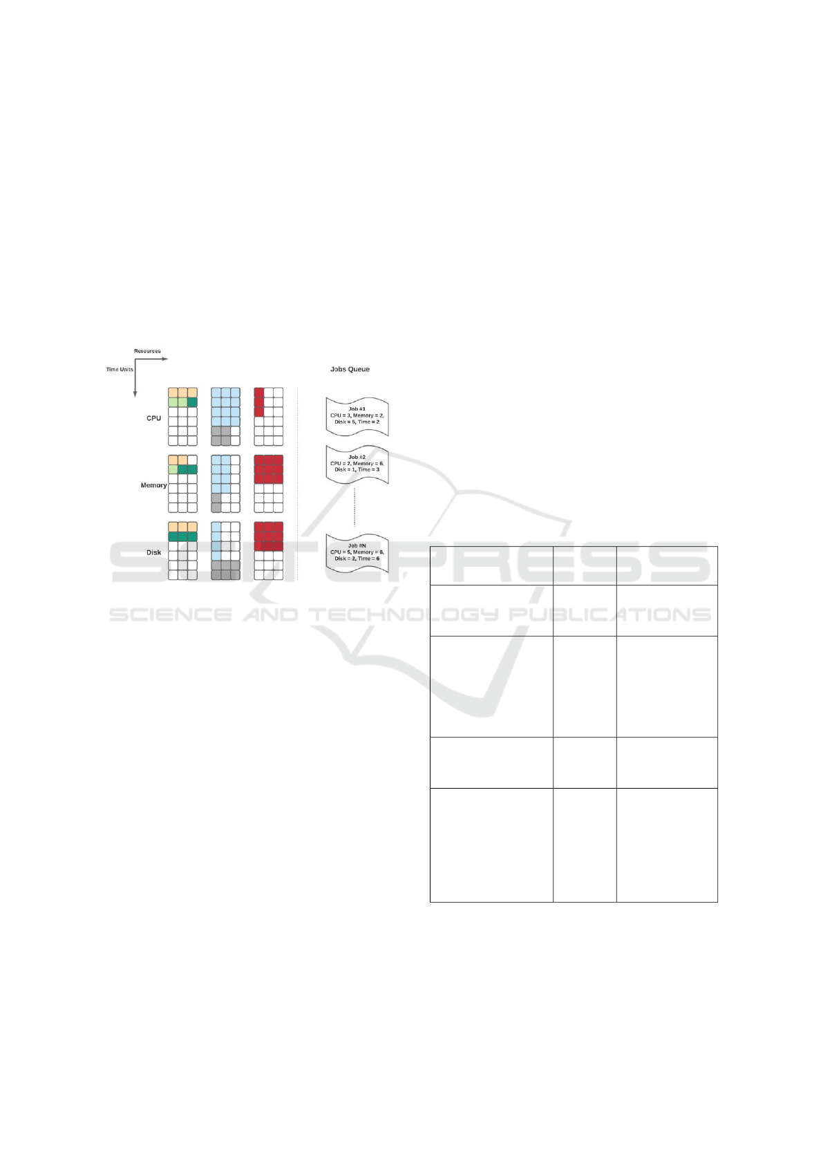
sentation of a single state, at a given time is provided
in Figure 1.
Figure 1: Environment State Representation - The vertical
axis indicates how many time units the algorithm can look
into the future. Jobs that require a longer processing time do
not meet the requirements and are therefore dropped. The
example consists of three different solver resource types
(CPU, memory and disk), with three similar instances con-
figured to run tasks in parallel and six time units available
for scheduling. There are N jobs waiting in the queue, each
with resource requirements listed. The colored boxes in
the solver instances indicate six jobs that are currently in
progress. For example, the red task in progress is estimated
to take three units of time to complete and has the follow-
ing resource requirements: one unit of CPU, three units of
memory, and three units of disk.
We assumed one key requirement: the framework
and its systems needs to be stable and easily adaptable
to new scenarios. After conducting several experi-
ments, we have chosen Keras, Tensorflow and Keras-
RL (Abadi et al., 2016) as primary tools, the later one
being a fullyfledged library that helped us implement
common and stateof- the-art reinforcement learning
methods: Deep Q-Networks (DQN), Double DQN,
Dueling DQN, Deep Deterministic Policy Gradient
(DDPG) and SARSA. We also used Keras and Ten-
sorflow as a pair for developing the supervised solu-
tion, based on pure Convolutional Neural Networks
(CNNs).
The entire code base is packaged to be easily mod-
ified and improved later, in future iterations. Also, a
dashboard was a must in order to extract metrics from
simulations and actual results or conclusions. All
reinforcement learning strategies were packed into
agents, but for easier testing we had to convert heuris-
tics and supervised methods to a similar structure,
so we have added a wrapper for them which can
be plugged in easily into the main structure of the
project.
5 METHODS
5.1 Dataset and Environment Setup
During the evaluation of the methods, we worked with
multiple datasets published, out of which we gained
insights by observing the common parameters and
setups. Table 1 and Table 2 describe the set of
parameters and their ranges used by our generated
dataset when training and evaluating the scheduling
algorithms within the framework.
Table 1: Parameters - Environment.
Value Observations
Total number of tasks
generated in a
simulation episode
1.000.000
A fixed value
was used
for simplified
charts & results
Max. Arrival Time
1440 units
The maximum
time
between two
consecutive
arrivals of a task.
This simulates the
number of minutes
in one day.
Max. Processing Time
5 units
Maximum
processing
time needed for
any task.
Max. Due Time
30 units
Maximum due
time
for finishing any
generated task
after arriving in
the system.
Must be higher
than required
processing time.
As stated before, all experiments will be fo-
cused on a simulation of a cloud computing environ-
ment, such as Google Cloud Platform (GCP), AWS
Lambda, or Azure Functions.
Task Scheduling: A Reinforcement Learning Based Approach
951

Table 2: Parameters - Tasks.
Metric Value Observations
Max. CPU
Units
3 units
The maximum
number of CPU
cores required
by any task.
At least one
CPU core is
required.
Max. RAM
Units
8 units
The maximum
RAM units
cores required
by any task.
At least one
CPU core is
required.
Max. Disk
Memory Units
10 units
Maximum due time
for finishing any
generated task
after arriving in
the system.
Must be higher
than required
processing time.
5.2 Neural Network Architecture
The neural network architecture (Table II) used in
the actual training steps of the reinforcement algo-
rithm and supervised method is based on convolu-
tional networks. This choice is motivated by the
way our environment is designed. Such an architec-
ture can successfully detect cases where systems are
overloaded or unbalanced, similar to playing multiple
Tetris games simultaneously, with some games par-
allelized (instances) and some directly connected (re-
sources).
The network configuration presented in Table 3
is classic, with some tweaks that we’ve made during
experiments:
• Convolutional dropout layers are calibrated to
avoid overfit but still passing most of the data to
next layers with a dropout rate of 30% (0.3).
• Fully connected layers are prone to overfit early,
so a more aggressive dropout strategy was neces-
sary, 50% being the rate resulted from multiple
simulations.
• The output layer is dynamic, based on the type
of system we are dealing with. This can be con-
sidered a little drawback, but most of the time in
a production environment we are dealing with a
fixed or low varied number of workers that are
not swapped every time. For example, 4 paral-
lel workers with a queue size of 30 will define a
total pool of 150 possible actions.
Table 3: Network Setup & Parameters.
Layer Value Details
Convolution #1
Output size:
60 x 260
Size: 3 x 3
Stride: 1
Activation Function:
Leaky ReLU
Avg Pooling #1
Output size:
30 x 130
Size: 2 x 2
Stride: 2
Dropout #1
0.3 dropout
rate
Convolution #2
Output size:
30 x 130
Size: 3 x 3
Stride: 1
Activation Function:
Leaky ReLU
Avg Pooling #2
Output size:
15 x 65
Size: 2 x 2
Stride: 2
Dropout #2
0.3 dropout
rate
Flatten
Required for further
fully connected
layers.
Fully Connected #1
Output 1 x 1
512 cells
Activation Function:
Leaky ReLU
Dropout #3
0.5 dropout
rate
Fully Connected #2
Output 1 x 1
256 cells
Activation Function:
Leaky ReLU
Dropout #4
0.5 dropout
rate
Fully Connected #3
Output 1 x 1
128 cells
Activation Function:
Leaky ReLU
We’ve used Leaky ReLU as main activation func-
tion due to gradients sparsity (Xu et al., 2015).
The configuration proposed above is used for all
the implemented and evaluated techniques.
5.3 Reward Function
Each agent trained by the algorithm has a fixed ac-
tion space defined by the equation below, and ranging
from [1, action space size].
action space size = nr. solver instances ∗
waiting queue size
(1)
Intuitively, this action space representation comes
from the fact that at any step the agent must place
a task X, from the waiting queue, to one of solvers
available.
In contrast, the perfect reward function is more
difficult to obtain because it must be adapted for dif-
ferent scenarios and data set parameters. Thus, this
function needs to be adapted from one environment
specification to another. Considering this, we allow
users to contribute their own customized function in
addition to the default reward functions we propose.
In our method, we first computed a slowdown fac-
tor for each scheduled task, i.e., created a ratio be-
ICAART 2023 - 15th International Conference on Agents and Artificial Intelligence
952

tween the actual completion time of a task, C
i
(wait-
ing time + processing time P
i
) and the required pro-
cessing time. This choice reflects how quickly the
system can respond to new jobs and evaluate the fi-
nal performance. The raw reward value computed
for each episode follows next equation, which iterates
over all tasks in an episode and computes the rela-
tionship between the completion time and its expected
processing time.
episodeRewardRaw =
∑
n
i=1
P
i
C
i
n
(2)
By using the above reward formulation, our solu-
tion tries to avoid a bad behavior seen in some heuris-
tic strategies: orders with high processing time are
postponed for too long, so that the deadline is eventu-
ally reached too early. This reward can be treated as a
normalization strategy.
Another value considered in the episode reward is
the average time of service level agreement violations.
This value is calculated by taking the average of the
SLAs over the entire dataset after each episode. It is
obtained by tacking the difference between the total
completion time required and the due time.
SLA avg. time = processing time+
wait time − due time
(3)
Other factors added to the reward used:
• Compact distribution of occupancy among
solvers, with high variance leading to negative
rewards. This factor will be called Compactness
Score (CS).
CS =
∑
w∈Workers
(Occup(w) − Occup)
2
n
(4)
Where Occup(w) represents the occupancy factor
(0-1) for the resources allocated on worker w at
the current timestep, while Occup is the mean of
the occupancy factors.
Occup(w) =
∑
w∈Resources
NO(r, w)
Total(r, w)
(5)
Where NO(r, w) (NumOccupied) represents the
number of cells of resource type r used currently
by worker w, while Total(r, w) represents the total
number of physically usable cells of type r in w.
• Total number of tasks that exceed the deadline or
fall out of our queue, describing negative rewards.
NED =
∑
timestep∈EpisodeSteps
NE(timestep)
(6)
NED(T) =
∑
task∈WaitingTasks
1
deadline(task)<T
(7)
• Total number of scheduled tasks in a time step,
treated as a major positive reward. This means
that a strategy is capable to fit as many tasks as
possible in a single timeframe.
NSS =
∑
timestep∈EpisodeSteps
NumScheduled(timestep)
(8)
We can further summarize the actual reward for-
mula:
episodeReward = episodeRewardRaw + δ ∗ NSS
− α ∗ SLA avg. time − β ∗ CS − γ ∗ NED
(9)
6 EVALUATION
6.1 Training Sessions & Evaluation
Details
The method used in our experiments to tune hyperpa-
rameters is grid search. We limit ourselves to listing
the parameters and the ranges chosen, and to making
some brief observations to help with further develop-
ment to serve as reference:
• Number of Episodes – A sign of convergence
was reached after a higher number of episodes
(more than 200). Deeper neural networks require
more than 1000 episodes, for example 5+ con-
volution layers. The ideal number of episodes is
around 500 for our basic model.
• Epsilon & Decay – Each algorithm was tested
with a classical value of 0.99 for the start epsilon,
0.99 for the decay rate and 0.1 for the minimum
epsilon. The last set delay is reached after almost
230 episodes, based on the next equation:
epsilon =
max(epsilon
initial
∗ epsilon
episodeIndex
decay
, epsilon
min
)
(10)
• Batch Size – Varies between 32 and 256, with the
ideal value being 64 for faster training sessions
and a reasonable result.
• Experience Replay Collection Size – This value
was a crucial factor as we cannot capture all pos-
sible combinations of actions, states, and rewards.
The ideal value is 100.000, but this comes at
a price when it comes to memory usage during
training sessions, which is a real issue in cloud en-
vironments. Nearly 50GB RAM of memory was
used for training our largest model. GPU acceler-
ation proves useful as the average time per epoch
is between 3 and 5 minutes. Larger cases require
Task Scheduling: A Reinforcement Learning Based Approach
953

over 500.000 large arrays, but this should be used
for local development, not an actual product.
• Learning Rate – A high learning rate of over 0.1
is not desired for our case, as it only leads to
a large fluctuation in rewards, not a constant in-
crease. Our choice fell on a value between 0.001
and 0.025. The final choice of 0.025 learning was
obtained with fine tuning and for this specific hy-
perparameter grid search we’ve used grid search.
• Reward Factors – In our simulation, we used the
following constant values:
Table 4: Reward factors.
α β γ δ
1.0 1.0 0.25 0.25
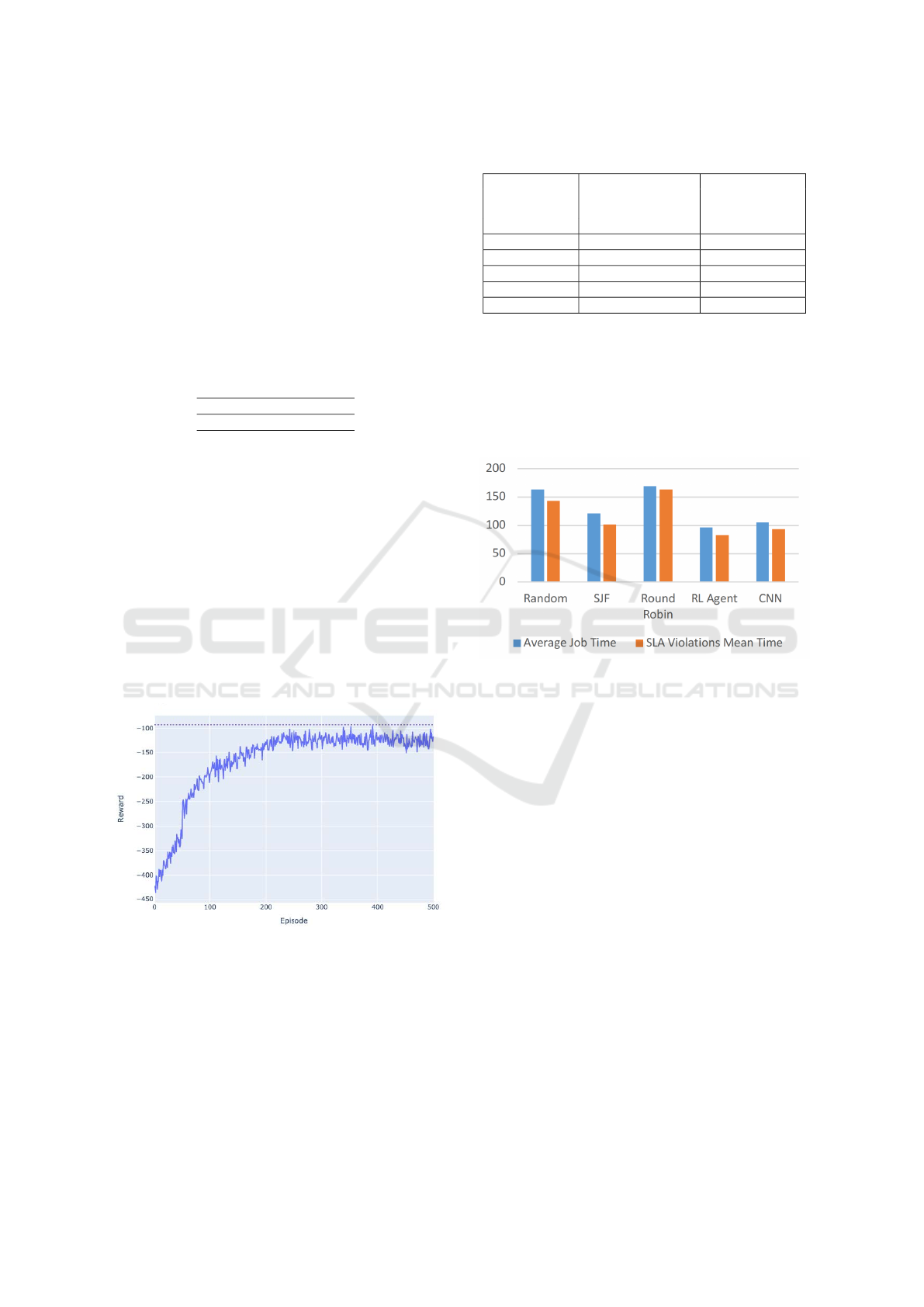
6.2 Results
Choosing a reasonable set of good parameters ensured
convergence over time and consistency (plateau re-
gion), which means that our agent is stable (Figure
2). We’ve concluded that reinforcement learning en-
riched with neural networks is a viable solution for
scheduling tasks.
A good curve of reward values and a point of con-
vergence was reached after an average of 250-300
episodes and 50.000 array sizes of experience replay.
We determined a moderate learning rate of 0.01 as be-
ing the best suitable for the method developed during
this research.
Figure 2: Best agent (reinforcement learning - DQN with
CNN) and reward obtained over time.
Although the results are encouraging, we need to
compare them with other approaches.
First, we compare the developed framework pre-
sented in the research with three different meth-
ods based on heuristics, randomness and supervised
learning, where each scenario is tested on normal and
uniform data distributions.
Table 5: Results.
Algorithm Average Job Time
SLA Violations
Mean Time
Random
163 Units 143 units
SJF
121 Units 101,5 units
Round Robin
169,5 Units 163 units
RL Agent
96 Units 82,5 units
RL + CNN
105,5 Units 93 units
Round Robin proved to be an inefficient strategy
of scheduling due to lack of perceptiveness. Most use
cases focus on quickly changing resources allocated,
from one task to another (Figure 3). Our candidate
method has proven to optimize the actual flow by al-
most 25%, regardless of the distribution or scenario
of the selected tasks.
Figure 3: RL Agent vs. CNN vs. Heuristics vs. Random.
Finally, we compared our agent with the state-of-
the-art solution DeepRM, which is also based on a
similar reinforcement learning approach, but on a dif-
ferent implementation stack of algorithms and neural
network architecture. Our method proved to achieve
slightly better results, . On the architectural side of the
things, we decouple the environment simulation and
definition from the methods used to train the agents.
Both concepts can vary in parallel, giving the possi-
bility of easy customization and faster prototyping of
new research ideas.
7 CONCLUSIONS
In summary, this research focuses on developing
and building a framework for several task schedul-
ing cases. Job Shop Scheduling related problems can
be formulated in different ways, with different con-
straints and conditions that involve one or more re-
sources in the computation. Therefore, it is important
to understand how difficult it is to develop an ultimate
solution that optimizes all possible workflows. Rein-
ICAART 2023 - 15th International Conference on Agents and Artificial Intelligence
954

forcement learning has already proven that it can de-
tect general patterns and improve results towards hu-
man capabilities. In this work, we presented a method
to develop an RL agent that outperforms classical so-
lutions or similar studies performed with state-of-the-
art machine learning based solution from the litera-
ture. The dataset generator we have created could also
be important for the research community, as there is
certainly a gap at present when it comes to experi-
menting different methods in an appropriate way and
quickly. One way to use this generator in the future
could be to create and fix some well-parameterized
datasets and then compare different methods using the
same data.
REFERENCES
Abadi, M., Barham, P., Chen, J., Chen, Z., Davis, A., Dean,
J., Devin, M., Ghemawat, S., Irving, G., Isard, M.,
Kudlur, M., Levenberg, J., Monga, R., Moore, S.,
Murray, D. G., Steiner, B., Tucker, P., Vasudevan, V.,
Warden, P., Wicke, M., Yu, Y., and Zheng, X. (2016).
Tensorflow: A system for large-scale machine learn-
ing. In 12th USENIX Symposium on Operating Sys-
tems Design and Implementation (OSDI 16), pages
265–283.
Asghari, A., Sohrabi, M., and Yaghmaee, F. (2020). Online
scheduling of dependent tasks of cloud’s workflows to
enhance resource utilization and reduce the makespan
using multiple reinforcement learning-based agents.
Soft Computing, 24:1–23.
Brockman, G., Cheung, V., Pettersson, L., Schneider, J.,
Schulman, J., Tang, J., and Zaremba, W. (2016). Ope-
nai gym.
Jang, B., Kim, M., Harerimana, G., and Kim, J. W. (2019).
Q-learning algorithms: A comprehensive classifi-
cation and applications. IEEE Access, 7:133653–
133667.
Konda, V. and Tsitsiklis, J. (2001). Actor-critic algorithms.
Society for Industrial and Applied Mathematics, 42.
Letchford, A. and Lodi, A. (2007). The traveling salesman
problem: a book review. 4OR, 5:315–317.
Li, F. and Hu, B. (2019). Deepjs: Job scheduling based
on deep reinforcement learning in cloud data center.
In Proceedings of the 4th International Conference on
Big Data and Computing, ICBDC ’19, page 48–53,
New York, NY, USA. Association for Computing Ma-
chinery.
Li, Y.-F., Tu, S.-T., Yan, Y.-N., Chen, Y.-C., and Chou, C.-
H. (2021). The utilization of big data analytics on food
delivery platforms in taiwan: Taking uber eats and
foodpanda as an example. In 2021 IEEE International
Conference on Consumer Electronics-Taiwan (ICCE-
TW), pages 1–2.
Mao, H., Alizadeh, M., Menache, I., and Kandula, S.
(2016). Resource management with deep reinforce-
ment learning. In Proceedings of the 15th ACM Work-
shop on Hot Topics in Networks, HotNets ’16’, page
50–56, New York, NY, USA. Association for Comput-
ing Machinery.
Mnih, V., Kavukcuoglu, K., Silver, D., Graves, A.,
Antonoglou, I., Wierstra, D., and Riedmiller, M.
(2013). Playing atari with deep reinforcement learn-
ing.
Nazari, M., Oroojlooy, A., Snyder, L. V., and Tak
´
a
ˇ
c, M.
(2018). Reinforcement learning for solving the vehi-
cle routing problem.
Rummery, G. and Niranjan, M. (1994). On-line q-
learning using connectionist systems. Technical Re-
port CUED/F-INFENG/TR 166.
Schmidt, R. M. (2019). Recurrent neural networks (rnns):
A gentle introduction and overview.
Schulman, J., Wolski, F., Dhariwal, P., Radford, A., and
Klimov, O. (2017). Proximal policy optimization al-
gorithms.
Shyalika, C., Silva, T., and Karunananda, A. (2020). Re-
inforcement learning in dynamic task scheduling: A
review. SN Computer Science, 1:306.
Silver, D., Lever, G., Heess, N., Degris, T., Wierstra, D.,
and Riedmiller, M. (2014). Deterministic policy gra-
dient algorithms. 31st International Conference on
Machine Learning, ICML 2014, 1.
Song, P., Chi, C., Ji, K., Liu, Z., Zhang, F., Zhang, S.,
Qiu, D., and Wan, X. (2021). A deep reinforcement
learning-based task scheduling algorithm for energy
efficiency in data centers. In 2021 International Con-
ference on Computer Communications and Networks
(ICCCN), pages 1–9.
Sutton, R. S. and Barto, A. G. (2018). Reinforcement Learn-
ing: An Introduction. A Bradford Book, Cambridge,
MA, USA.
Tassel, P., Gebser, M., and Schekotihin, K. (2021). A rein-
forcement learning environment for job-shop schedul-
ing.
Xu, B., Wang, N., Chen, T., and Li, M. (2015). Empiri-
cal evaluation of rectified activations in convolutional
network.
Ye, Y., Ren, X., Wang, J., Xu, L., Guo, W., Huang, W.,
and Tian, W. (2018). A new approach for resource
scheduling with deep reinforcement learning.
Task Scheduling: A Reinforcement Learning Based Approach
955