
Efficient Deep Learning Ensemble for Skin Lesion Classification
David Due
˜
nas Gaviria
1 a
, Md Mostafa Kamal Saker
2 b
and Petia Radeva
3,4 c
1
Facultat d’Informatica de Barcelona, Universitat Polit
`
ecnica de Catalunya, Carrer de Jordi Girona 31, Barcelona, Spain
2
Department of Engineering Science, University of Oxford, Headington OX3 7DQ, Oxford, England, U.K.
3
Department of Mathematics and Computer Science, Universitat de Barcelona, Gran Via de les Corts Catalanes 585,
Barcelona, Spain
4
Computer Vision Center, Bellaterra, Barcelona, Spain
Keywords:
Skin Cancer, Melanoma, ISIC Challenge, Vision Transformers.
Abstract:
Vision Transformers (ViTs) are deep learning techniques that have been gaining in popularity in recent years.
In this work, we study the performance of ViTs and Convolutional Neural Networks (CNNs) on skin le-
sions classification tasks, specifically melanoma diagnosis. We show that regardless of the performance of
both architectures, an ensemble of them can improve their generalization. We also present an adaptation
to the Gram-OOD* method (detecting Out-of-distribution (OOD) using Gram matrices) for skin lesion im-
ages. Moreover, the integration of super-convergence was critical to success in building models with strict
computing and training time constraints. We evaluated our ensemble of ViTs and CNNs, demonstrating that
generalization is enhanced by placing first in the 2019 and third in the 2020 ISIC Challenge Live Leaderboards
(available at https://challenge.isic-archive.com/leaderboards/live/).
1 INTRODUCTION
Skin cancer has become a major public health con-
cern; between 2 and 3 million non-melanoma skin
cancers occur each year and 132 thousand melanoma
worldwide, claiming more than 20 thousand lives in
Europe alone each year, and 57 thousand worldwide,
based on the most recent (Forsea, 2020), (ACS, 2022).
Melanoma is the deadliest form of skin cancer (WHO,
2017), and a later stage of melanoma diagnosis has
been linked to a significant increase in mortality rate.
As medical professionals and patients’ needs for
technology have increased, so have the demands for
automated skin cancer diagnosis (Chang et al., 2013).
In response, current research has produced automated
skin cancer diagnostic tools that perform on par with
dermatologists who rely mostly on visual diagnosis,
dermoscopic analysis, or invasive biopsy, along with
a histopathological study. Nonetheless, Deep Learn-
ing (DL) has revolutionized the field of computer
vision in recent years with the resurgence of Neu-
ral Network (NNs) architectures (Belilovsky et al.,
2019). Convolutional Neural Networks (CNNs) have
a
https://orcid.org/0000-0002-4869-668X
b
https://orcid.org/0000-0002-4793-6661
c
https://orcid.org/0000-0003-0047-5172
become the dominant DL technique in this field, due
in large part to their success in the ImageNet Large
Scale Visual Recognition Challenge (ILSVRC) (Rus-
sakovsky et al., 2015). However, there are a num-
ber of other DL techniques that have been gaining in
popularity in recent years. Particularly, Vision Trans-
formers (ViTs) (Dosovitskiy et al., 2021), which cor-
respond to a type of transformer that is specifically
designed for computer vision tasks. Transformers are
a type of DL model based on the attention mech-
anism and have proved successful in a number of
natural languages processing tasks (Vaswani et al.,
2017). Although considerable research has been done
on the use of ViTs for medical image classification,
see (Chen et al., 2021; Sarker et al., 2022), robust-
ness against skin lesions in generalization has not yet
been explicit. This is generally the case because the
training and testing data for many closed-world tasks
are taken from the same distribution. However, in the
ISIC 2019 dataset particularly, the effect of an outlier
class poses a significant challenge for ViTs in compar-
ison to traditional CNNs. Hence, the aim of this study
is to answer: How useful is the incorporation of ViTs
in classification for skin cancer detection, particularly
melanoma, in comparison to CNNs?
Skin lesion classification using ViTs and CNNs
Gaviria, D., Saker, M. and Radeva, P.
Efficient Deep Learning Ensemble for Skin Lesion Classification.
DOI: 10.5220/0011816100003417
In Proceedings of the 18th International Joint Conference on Computer Vision, Imaging and Computer Graphics Theory and Applications (VISIGRAPP 2023) - Volume 5: VISAPP, pages
303-314
ISBN: 978-989-758-634-7; ISSN: 2184-4321
Copyright
c
2023 by SCITEPRESS – Science and Technology Publications, Lda. Under CC license (CC BY-NC-ND 4.0)
303

shares the same goal of detecting skin disease lesions
by using image-level and patient-level data. Thus, it
makes sense to test their performance together using
a common ensemble. As a result, the contributions of
this study are as follows:
• Focusing on the main goal of skin disease clas-
sification problem, we propose a robust model,
based on an ensemble comprising a wide range of
model architectures, including top accuracy ViTs
and popular CNNs. Our model outperformed the
state of the art in the 2019 ISIC competition.
• Instead of using a loss function normalized to take
into account imbalanced data during the training,
our model demonstrates that the skin lesion diag-
nosis represented by its inherent imbalanced data
can be handled by re-scaling the decision thresh-
old at model inference.
• Our model shows improvements in the Gram-
OOD* method for the detection of OOD samples
in the ensemble predictions.
• We employed the super-convergence phe-
nomenon which allowed for a larger number of
individual experiments, despite computing and
time constraints.
• Finally, providing a consistent validation pipeline,
we demonstrate that applying domain-dependent
transformations is crucial in a data augmentation
regime achieving top performance with our com-
bined ViTs and CNNs ensemble model.
The following study is arranged as follows: Sec-
tion 2 goes over our model description and imple-
mentation processes training various ViTs and CNNs
models used along with details on the data used. Sec-
tion 3 displays and summarizes the results acquired
along with the discussion on the validation approach.
Finally, last section gives conclusions of the study
given and future research lines to be pursued.
2 METHODOLOGY
Here we introduce our new method for skin lesion
classification, which was able to demonstrate robust-
ness in generalization by scoring first in the 2019 ISIC
Challenge and third in the 2020 ISIC Challenge, de-
spite computing and training-time limitations. Over-
all, the following contributions made it possible to
achieve such a position: a diversity provided by ViTs
and CNNs ensemble; handling the imbalanced data
problem, through re-scaling the model’s predictions,
by using the output class probabilities; improvements
in OOD detection through an adaptation of the Gram-
OOD* method; super-convergence through the usage
of OneCycle LR in conjunction with AdamP opti-
mizer, and domain-dependent image augmentation,
for learning credible representations of skin lesions.
2.1 A New Ensemble of Deep Learning
Models for Skin Lesion
Classification
A variety of state-of-the-art ViTs and CNNs were ex-
plored in our work in order to study their jointly be-
haviour in the context of skin lesion diagnosis. After
a thorough analysis on the state-of-the-art DL mod-
els, we concluded that the highly complex problem of
skin lesion classification requires an ensemble of ro-
bust performing models. Hence, here we propose an
ensemble that consists of:
• Data-efficient Image Transformer (DeiT) (Tou-
vron et al., 2021a) - a type of ViT trained using
a teacher-student strategy specific to transformers
relying on a distillation token, it ensures that the
student learns from the teacher through attention.
• EfficientNets (Tan and Le, 2019), trained on
Noisy-Student weights (Xie et al., 2020) and us-
ing a scaling technique to equally scale the net-
work’s width, depth, and resolution using a set of
predefined scaling coefficients.
• ConvNeXt (Liu et al., 2022b), resulting in a hy-
brid model lacking attention-based modules that
adapt a ConvNet towards the design of a hierar-
chical Swin transformer.
The diagram of the pipeline is depicted in Figure
1, which shows the use of both ViTs and CNNs. Thus,
the final ensemble in the training pipeline (a) shows in
blue and green the CNNs and ViTs respectively, be-
ing trained using the dataset images with the external
datasets (see Figure 4). The orange line, on the other
hand, represents the pipeline that was used to train
the network to add the metadata. Afterwards, model
selection is performed at the training phase, determin-
ing the correlation of each model’s training and vali-
dation prediction to filter out overfitting models. (b)
indicates the inference pipeline, which consisted of
generating output predictions using Test Time Aug-
mentation (TTA) (Shanmugam et al., 2020) with a
similar augmentation regime than in training (Except
CutOut). Moreover, creating the ensemble by aver-
aging the model predictions and performing thresh-
olding on the resulting predictions. Finally, Gram-
OOD* adaptation improves OOD detection by replac-
ing the method’s generated outlier class predictions in
the previous ensemble.
VISAPP 2023 - 18th International Conference on Computer Vision Theory and Applications
304
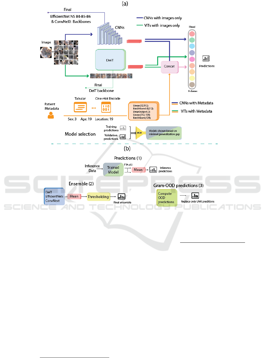
Figure 1: Diagram of the pipeline of our model. (a) depicts the training pipeline and (b) inference pipeline. The final ensemble
uses an average of models trained with only images, and both images and metadata. The inference pipeline shows the output
predictions in three stages.
2.2 Model Selection Based on Mean
Correlation Matrix
The goal of our strategy inspired in (Nikita Kozodoi,
2020) is to exclude models whose mean correlation of
predictions revealed a significant gap between train-
ing and validation predictions among the different
models in order to select consistent and stable models.
The basic idea is to find the correlation between the
training predictions and in the correlation of the vali-
dation predictions for the individual models to assess
the divergence between training and validation based
on the correlations of each pair of models. Equations
(1) and (2) indicate the correlation coefficients ρ
i j
for
each pair of models i and j forming a stacked matrix
for the training x
tr
and validation x
v
data:
ρ
i j
tr
=
|C|
∑
c=1
∑
|c|
k=1
(x
i
tr,k
− µ
i
tr,c
)(x
j
tr,k
− µ
j
tr,c
)
σ
i
tr,c
∗ σ
j
tr,c
(1)
ρ
i j
v
=
|C|
∑
c=1
∑
|c|
k=1
(x
i
v,k
− µ
i
v,c
)(x
j
v,k
− µ
j
v,c
)
σ
i
v,c
∗ σ
j
v,c
, (2)
where x
i
tr,k
are the training data output of model i of
class c, x
i
v,k
are the validation data output of model i of
class c, µ
i
tr,c
and σ
i
tr,c
are the mean and the variance of
the training data output of model i of class c, µ
i
v,c
and
σ
i
v,c
are the mean and the variance of the validation
data output of model i of class c, |C| is the number of
classes and |c| is the number of data in class c.
Equation (3) shows the Mean Correlation Matrix
(MCM) which corresponds to the arithmetic mean
computation of the absolute gap difference of the
model-pair-wise correlations:
{MCM
i j
} =
ρ
i j
v
− ρ
i j
tr
. (3)
Note that the MCM matrix has dimensions |M| ×
|M| where |M| is the number of models. In order to
find the first T models with minimum gap, we sum
Efficient Deep Learning Ensemble for Skin Lesion Classification
305

the differences corresponding to each model (sum-
ming the rows of the MCM matrix), sort them and
keep the first T models with minimum values:
{sort{
1
|M|
|M|
∑
i=1
MCM
i j
}}
j=1,...,T
.
Note that a greater gap MCM indicates that the
model predictions behave differently between training
and validation data. Therefore, it is possible that a
feature on which this model largely depends, has a
different distribution between training and validation
data, causing it to overfit the training data and affect
its generalization. Section 3.6 proves the importance
of the MCM in the ensemble’s model selection.
2.3 OOD with a Modified Gram-OOD*
Gram-OOD (Sastry and Oore, 2019) is a robust ap-
proach that relies on intermediate feature activations
to treat data with OOD samples, with the benefit of
not requiring additional data. In order to detect ab-
normalities, the original method computes layer-wise
correlations using Gram-Matrices:
G
p
l
= F
p
l
F
p⊤
l
, ∆( ˘x) =
∑
δ
l
( ˘x
c
)
E
v
[δ
l
]
. (4)
where c corresponds to the class assigned by the clas-
sifier, ˘x represents the total deviation of a new image,
F
l
corresponds to the activation of layer l, L - the total
number of layers, p is a parameter, E
v
[δ
l
] is the ex-
pected deviation from the validation data at layer δ
l
.
In other words, to highlight the prominent features,
Equation (4) computes high-order Gram-Matrices of
order p with F
l
corresponding to activations at layer l.
The first step is to compute the pair-wise correlation
between the obtained feature maps, both in convolu-
tional layers and activation layers. Next, the layer-
wise deviations from the gram matrices are computed
so that it is possible to know how much a sample de-
viates from the max/min values over the training data.
Finally, the original method computes the total devi-
ation by summing its layer-wise deviation across all
layers. In Equation (4), the expected deviation from
the validation data E
v
[δ
l
] is computed using the val-
idation set, avoiding the need for OOD datasets, in
contrast to techniques such as (Liang et al., 2018),
which need both in-distribution and OOD datasets.
The Gram-OOD* (Pacheco et al., 2020) considers
only the activation layers adding an extra normalizing
layer between the pair-wise correlations and the layer-
wise variances. The normalization procedure is:
˜
G
p
l
=
ˆ
G
p
l
− min(
ˆ
G
p
l
)
max(
ˆ
G
p
l
) − min(
ˆ
G
p
l
)
(5)
In this paper, we propose a modified version of the
Gram-OOD* (Pacheco et al., 2020) in which the fea-
ture maps are computed from the convolutional lay-
ers, instead of the activation layers. In this way, we
retain critical features from the pair-wise correlations
and apply the normalization procedure (see Equation
(5)) with a substantially reduced computational cost
without sacrificing generalization capacity.
2.4 Loss Function for Skin Lesion
Classification
As in many medical image datasets, data imbalance
is a common, yet challenging issue to be addressed
for model design and hyper-parameters optimization.
Most popular approaches, such as Weighted Cross
Entropy (WCE) (Aurelio et al., 2019), or Focal loss
(FL) (Lin et al., 2020) have been widely used to
address it. However, performance can improve by
means of the regular Cross Entropy (CE) properly re-
scaling the output predictions at inference as follows:
CE = −
|C|
∑
c=1
y
o,c
log(p
o,c
) (6)
where |C| is the number of classes, y as the binary
indicator (groundtruth) if class label c is correct for
observation o, and p is the predicted probability ob-
servation that o is of class c. The improvement is
achieved by re-scaling the output class probabilities
with the method known as thresholding (Buda et al.,
2018). This approach applied in (Steppan and Hanke,
2021) has been demonstrated to significantly improve
the performance in imbalanced datasets by a class
probability distribution approximation. (Richard and
Lippmann, 1991) has shown that NNs classifiers de-
rive Bayesian a posteriori probabilities, where they
are computed for each class by their frequency in
the imbalanced dataset. In other words, the thresh-
old T (x) is computed given the output for class c for
a datapoint x that implicitly corresponds to the con-
ditional probability in Equation (7), where |c| is the
number of unique training and validation instances in
class c and p(x) is considered constant assuming all
data have the same probability to be selected:
T (x) = p(c|x) =
p(c)p(x|c)
p(x)
, p(c) =
|c|
∑
|C|
k=1
|c
k
|
, (7)
where p(x|c) is the output of the softmax layer and
|c
k
| is the number of instances of class c
k
. Thus, de-
pending on the datasets that are considered, the re-
scaling made by the class prior will change.
VISAPP 2023 - 18th International Conference on Computer Vision Theory and Applications
306
3 VALIDATION
In this section, we discuss the datasets and their
preparation, followed by the main ensemble setting,
and evaluation metrics. Furthermore, we illustrate
the experimental results and discussions showing the
effect of the super-convergence, data augmentation,
OOD and the imbalanced data methods followed by
the final results on both challenges datasets from ISIC
2019 and ISIC 2020.
3.1 Skin Lesion Dataset Description
At the image level, there are 9.1 GB worth 25,331
dermoscopic images available for training in 8 dif-
ferent classes. This information was obtained from
the Memorial Sloan Kettering Cancer Center, the
BCN 20000 dataset from the Department of Derma-
tology, Hospital Clinic de Barcelona (Combalia et al.,
2019) and the HAM10000 dataset from the Depart-
ment of Dermatology, Medical University of Vienna
(Tschandl et al., 2018). Table 1 shows the nine classes
used for the diagnosis in the challenge and Table 2
shows the distribution of the external datasets. Like-
wise, the test dataset comprised 8,239 images with
the extra outlier class that was not represented in the
training data. Aside from the images, the collection
includes metadata such as the patient’s age and sex as
well as the location of the individual skin lesion.
ISIC 2020 dataset (Rotemberg et al., 2021) is
composed of 23 GB worth 33,126 images of different
resolutions for training and 10982 for the test set. A
total of 2056 patients was gathered for this dataset at
various locations around the world. In contrast to the
2019 dataset, the unknown class (UNK) accounted for
the majority of benign occurrences, including Cafe-
au-lait macule and atypical melanocytic proliferation
diagnosis, whereas the other three: melanocytic ne-
vus (NV), melanoma (MEL), and benign keratosis
(BKL), were also shared diagnosis within the 2019
dataset; the Basal cell carcinoma (BCC), Actinic ker-
atosis (AK), Squamous cell carcinoma (SCC), Vas-
cular lesion (VASC) and Dermatofibroma (DF) are
unique diagnosis from the 2019 dataset.
With the presence of an outlier class in the ISIC
2019 dataset, it was reasonable to experiment with
external data to attempt to increase training diversity
for the unknown and generalization of the remaining
classes. As an outline of (Steppan and Hanke, 2021),
the outlier class for training was addressed through
the usage of a subset of a collection of datasets, which
are shown in Table 2.
Table 1: Diagnosis distribution of 2019 and 2020 ISIC
datasets.
Diagnosis
2019 dataset
samples
2020 dataset
samples
NV 12875 (50%) 5193 (15%)
MEL 4522 (18%) 584 (2%)
BKL 2624 (10%) 223 (1%)
UNK 0 (0%) 27126 (82%)
BCC 3323 (13%) —
AK 867 (4%) —
SCC 628 (3%) —
VASC 253 (1%) —
DF 239 (1%) —
Total 25331 33126
Table 2: Diagnosis distribution for the external dataset.
External data
Dataset
7 point
(Walter et al., 2013)
PH2
(Giotis et al., 2015)
MED-NODE
(Giotis et al., 2015)
SD-198
(Sun et al., 2016)
Total
Number of images 1011 (13%) 200 (3%) 170 (2%) 5944 (78%) 7624
Total 7624
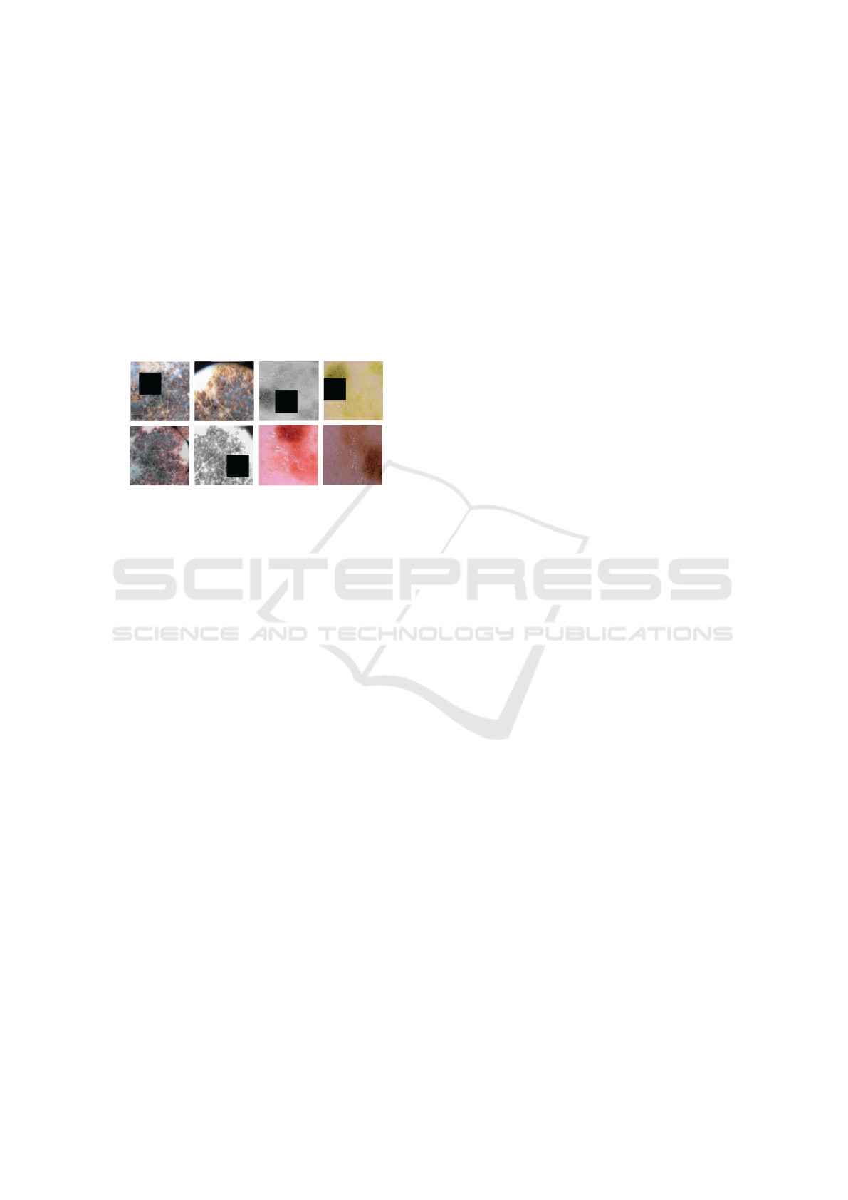
Figure 2: Preprocesssing of outlier images.
3.2 Data Preparation
The images in the dataset are all from different
sources, scanned at various resolutions and on the
same color space. However, some of them are com-
posed of microscope-like image cropping that were
detected as outliers, using the mean and standard de-
viation from the intensity values, and were prepro-
cessed to see whether they could result in an general-
ized improvement as (Gessert et al., 2020) stated. The
data handling first consisted of trimming and cropping
these microscope-lesion images, which were typically
high resolution. This process resulted in another im-
age with a lower resolution than the original, but with
the object of interest (skin lesion) clearly visible and
in greater detail. Figure 2 presents a few examples of
all the 9577 images determined as outliers.
Metadata missing values were addressed by intro-
ducing a new parameter unknown for the sex, age,
and anatomical location. In all, 3 sex features, 10
anatomical location features, and 19 sex features were
encoded utilizing a straightforward One-Hot encod-
ing procedure (Potdar et al., 2017). In this encoding,
Efficient Deep Learning Ensemble for Skin Lesion Classification
307
the matching attribute for each given output level is 1
while the remainder are all 0. A total of 32 stacked
features are used as input for the patient-level data.
Data Augmentation: Three popular methodolo-
gies from the literature were evaluated in order to dis-
cover a suitable data augmentation regime for such
real-world classification task; namely, AutoAugment
(Cubuk et al., 2019), RandAugment (Cubuk et al.,
2020) and AugMix (Hendrycks et al., 2020). Before
a selection, an adaptation of the customized standard
augmentation by (Ha et al., 2020) was studied in or-
der to find the most suitable augmentation technique
for newly unseen data.
Figure 3: Image augmentation employed: a standard aug-
mentation regime (random flip, rotation, brightness/contrast
and blur/gaussian noise) followed by a random and resized
crop strategy, CutOut of 30% image size, and gray and
color-jitter/hue-saturation changes.
Figure 3 shows the augmentation regime used
for all the models, which was based on the idea of
avoiding the deconstruction of features and patterns
in the melanocytic images described in the ABCD
rule (Ali et al., 2020): where skin lesion asymmetry
is a major indicator of malignant melanoma, in con-
trast to benign pigmented skin lesions, which are nor-
mally round and symmetric, melanomas spread un-
controllably. As a result, asymmetry, border, color,
and diameter are critical in developing a skin lesions
augmentation regime. Taking inspiration from Con-
trastive Learning (Chen et al., 2020) the composi-
tion of simple augmentations for learning good rep-
resentations, gray and color distortions were adopted.
Moreover, key to the locality of the augmentation
was a heavy cropping strategy, where random resized
crops were fed into the models followed by random
brightness and contrast changes including color jit-
ter, random flipping, random rotation, random scal-
ing, and random blur/noise/sharpen changes. Further-
more, CutOut (Devries and Taylor, 2017) was used
with one hole that was 30% the size of the image
and had a 50% chance of appearing. Finally, a cou-
ple of augmentation strategies, including microscopy-
crop and color constancy shades of grey as in (Gessert
et al., 2020), were explored, but yielded no benefits
and were therefore rejected.
Data Splitting: For the data splitting, the objec-
tive was to find a strategy that could work for both
model selection and hyper-parameter optimization.
The holdout method is the simplest strategy for eval-
uating a classifier and although it is not the best strat-
egy to exhaustedly assess the models on the whole
bulk of the data, it provides the advantage of imme-
diate experiments to determine the fundamental set-
tings for a robust classifier. To achieve generalization
on previously unseen data, it was vital to verify that
the training and validation were representative of the
full dataset. Hence, a stratified split based on the skin
lesion target class was necessary and based on the em-
pirical findings, a 90% to 10% split was decided.
Following a data-driven approach, adding external
data as in (Steppan and Hanke, 2021), demonstrated
a slight improvement for the outlier class. Therefore,
datasets described in Figure 4 (a) were used to feed
the models in order to reach diversity in our ensemble.
Moreover, in order to include metadata features, the
ISIC 2019 and ISIC 2020 datasets were both used for
training with a bulk of 57301 images. The stratified
split can be inspected in Figure 4 (b).
3.3 Model Training with LR Scheduler
and Selecting the Optimizer
We applied the procedure known as ”super-
convergence” (Smith and Topin, 2019) in paral-
lel throughout the whole model implementation,
given our GPU and training time limitations. The
”One-Cycle” Learning Rate (LR) policy proposed in
(Smith, 2018) makes use of this feature to address
the stochastic aspect of NNs by oscillating the LR
into greater and smaller values that aid in breaking
out of a plateau or local minima regions of the loss
functions. One cycle consists in two steps: one in
which LR increases from minimum to maximum
and the other in which it lowers from maximum
to minimum of the total number of epochs. In
super-convergence, networks are trained with high
LRs in an order of magnitude fewer iterations and
with better final test accuracy than when a constant
training regime is used. Super-convergence depends
critically on training with a single LR cycle and a
high LR. Furthermore, AdamP optimizer has been
shown to outperform the vast majority of Gradient
Descent Based optimizers in both computational cost
and performance on ImageNet (Heo et al., 2021). In
(Smith, 2018), the authors suggested testing any of
the 3e − 4, 1e − 4, and 3e − 5 as the maximum LR,
and in order to have uniformity for all tests, 3e − 4
was selected as the max LR.
We used the automatic scoring system detailed in
VISAPP 2023 - 18th International Conference on Computer Vision Theory and Applications
308
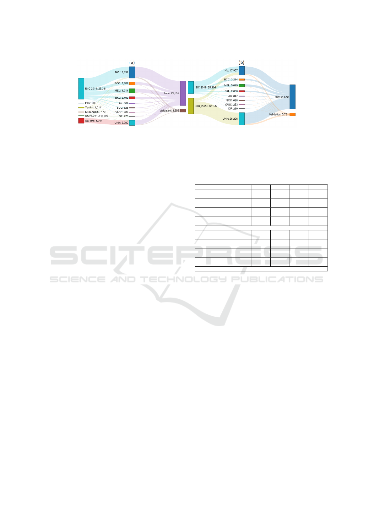
Figure 4: Skin Lesion Datasets Distribution for the external data is depicted in (a). It displays the 25,331 samples from the
ISIC 2019 as well as the contributions from the remaining external datasets and also indicates the splitting made for training
and validation. On the otther hand, (b) shows the metadata Skin Lesion Datasets Distribution for the 2019 and 2020 ISIC
datasets with 32,196 additional images. The contribution in each class is demonstrated here, along with the splitting approach
and 9:1 proportions for training and validation.
(Archive, 2019), for the 2019 ISIC Challenge to eval-
uate the performance of our models, Accuracy (ACC),
Balanced Multi-class Accuracy (BACC), BACC of
the validation set (Val BACC), sensitivity (SE), speci-
ficity (SP), Dice Coefficients (DI) and Area Under the
Curve (AUC) scores, receive operating characteristics
(ROC) curve.
3.4 Experimental Results
The results from the CNNs baseline in research (Step-
pan and Hanke, 2021) were adapted with the OneCy-
cle LR, given training and computational constraints.
Furthermore, a baseline of ViTs had to be obtained
in order to have a first look and comparison between
ViTs and CNNs in the skin lesion classification task.
The CNNs that were used for baseline comprise the
Efficient Nets (Tan and Le, 2019), Inception Resnet
V2 (Szegedy et al., 2017) and ResNeXt (Xie et al.,
2017). In the case of ViTs, we used as the baseline:
the basic ViT (Dosovitskiy et al., 2021), BEiT (Bao
et al., 2022), SwinT (Liu et al., 2021), and SwinTV2
(Liu et al., 2022a). Hence, the relevant models and
their performance are displayed in Table 3. Further-
more, initially, only images from the whole dataset
shown in Figure 4 were used. As a result, 29,639
training samples and 3296 validation images were
used with a 90-10 split from the PH2, 7-point crite-
rion, MED-NODE, SKINLV2-V1-2-3, SD-198, and
ISIC 2019 datasets; melanoma had 4914 samples for
baseline. With this particular setup, preliminary re-
sults show that CNNs defeat ViTs ensemble by a nar-
row margin. Additionally, the image size was multi-
resolution, and the EfficientNet B5 received the high-
est score of 0.483; Nonetheless, a variety of input
sizes for the ViTs backbones were needed in order to
adequately examine the results since ViTs lacks the
richness of scaled resolution.
Table 3: ISIC 2019 baseline scores. No data preprocessing,
duplicates removal or imbalance handling was performed.
Method # Params Image size Data usage Val BACC 2019 Score
SWSL ResNeXt-101 32x4d
(Yalniz et al., 2019)
54M 224 External 72.09% 0.429
Inception-ResNet-V2
(Szegedy et al., 2017)
56M 299 External 76.33% 0.433
EfficientNet B4
(Tan and Le, 2019)
19M 380 External 71.11% 0.424
EfficientNet B5
(Tan and Le, 2019)
30M 456 External 77.73% 0.483
CNNs baseline ensemble 0.496
ViT-L-16
(Dosovitskiy et al., 2021)
304M 224 External 75.73% 0.418
Swin-L-4
(Liu et al., 2021)
197M 224 External 73.02% 0.464
SwinV2-B-
(Liu et al., 2022a)
88M 256 External 74.56% 0.412
BeiT-B-16
(Bao et al., 2022)
87M 224 External 75.13% 0.403
ViTs baseline ensemble 0.482
3.5 ViTs and CNNs Ensemble Results
for 2019 ISIC Challenge
The 2019 ISIC Challenge, which contains an auto-
matic scoring system and 8,239 challenging images
in the test set, allowed for credibility in the evaluation
of our model’s generalization capabilities. The top
network results, which were obtained through an en-
semble of the ViTs and CNNs, are shown in Table 4.
Although BEiT-L is a powerful network for the Ima-
geNet dataset, as demostrated by (Bao et al., 2022),
it underperformed in all of the test results from ViTs
—with less than 0.500 for ISIC 2019 test score after
thresholding— and hence was omitted.
Furthermore, the ensemble predictions were cre-
ated using only the top six models from ViTs and
CNNs. Although the 384 image size was best for the
ViTs and the 380 image resolution was best for the
CNNs, the multi-resolution technique for ensemble
diversification allowed us to construct ensembles that
outperformed all individual models ranging from 224
to 528. The DeiT-D3 achieved a top validation score
of 91.73% and a high score of 0.593, indicating that
it has captured features not present in the other mod-
Efficient Deep Learning Ensemble for Skin Lesion Classification
309
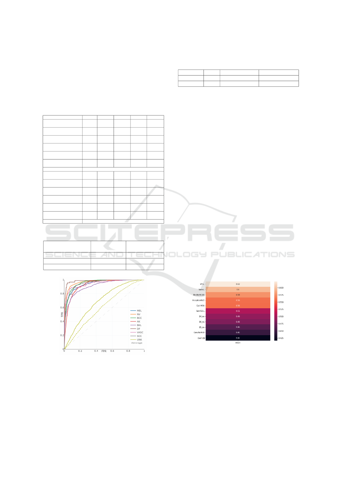
Table 4: BACC on training in ViTs and CNNs state-of-
the-art models. All hold-out splitting with 90 to 10% for
training and validation. We considered a heavy cropping
strategy with TTA 32 and only 10 epochs training via fine-
tuning. Values are given in % as BACC validation. The en-
semble was used as the average of all predictions from ViTs
and CNNs models. External refers to both the 2019 dataset
and the external datasets, and Meta means the 2019 dataset
and 2020 datasets training both the images and metadata. In
all cases, the 9 classes were used for prediction.
Method # Params Image size Data usage Val BACC 2019 Score
ViT-L-16
(Dosovitskiy et al., 2021)
26M 224
External 78.35% 0.514
Meta 83.56% 0.527
VOLO-D3
(Yuan et al., 2022)
306M 512
External 82.31% 0.512
Meta 85.36% 0.516
DeiT-D3
(Touvron et al., 2021a)
305M 384
External 89.97% 0.592
Meta 91.73% 0.593
CaiT-M-36
(Touvron et al., 2021b)
271M 380
External 84.29% 0.571
Meta 88.21% 0.589
Swin-L-4
(Liu et al., 2021)
197M 224
External 81.17% 0.526
Meta 83.87% 0.564
Swin-L-V2
(Liu et al., 2022a)
197M 384
External 86.10% 0.563
Meta 89.46% 0.610
ViTs Ensemble (ViTs above) 0.612
SWSL ResNeXt-101 32x4d
(Yalniz et al., 2019)
54M 224
External 75.73% 0.576
Meta 74.06% 0.579
Inception-ResNet-V2
(Szegedy et al., 2017)
56M 299
External 78.23% 0.586
Meta 78.24% 0.587
EfficientNet b4 NS
(Xie et al., 2020)
19M 380
External 83.66% 0.603
Meta 84.85% 0.630
EfficientNet b5 NS
(Xie et al., 2020)
30M 456
External 84.25% 0,604
Meta 85.94% 0.618
EfficientNet b6 NS
(Xie et al., 2020)
43M 528
External 85.99% 0.612
Meta 86.07% 0.630
ConvNeXt-B
(Liu et al., 2022b)
89M 384
External 85.91% 0.592
Meta 86.95% 0.594
CNNs Ensemble (CNNs above) 0.660
Table 5: Ensemble method used for the ViTs and CNNs.
Ensemble method
ViTs ensemble
2019 Score
CNNs ensemble
2019 Score
Rank of probabilities 0.611 0.647
Majority voting 0.542 0.603
Averaging 0.612 0.660
Figure 5: ROC curve with improvement AUC for the un-
known class.
els. CNNs, on the other hand, outperform ViTs for
the majority of individual ensembles in both external
and meta data. Finally, it was not intended to utilize a
brute force averaging strategy, as was the case in ear-
lier 2019 and 2020 ISIC submissions, hence a model
selection approach had to be used.
Table 6: Outlier class metrics comparison with the OOD
results for the top 1 in the 2019 ISIC live challenge.
Metric AUC AUC Sens >80% Average Precision
Unk 0.595 0.310 0.234
Unk-OOD 0.686 0.437 0.302
In order to take explicit care of OOD samples and
outperform the current methods in the challenges, we
used the modified Gram-OOD* to calculate the OOD
samples, as described in Section 2.3. Table 6 depicts
a comparison after the modified Gram-OOD* method
was applied, accounting for a slight improvement in
the AUC. We achieved AUC sensitivity higher than
80% and average precision of 0.686, 0.437 and 0.302,
respectively. Finally, the outlier class improvement is
shown in Figure 5. It illustrates the new ROC Curve
for the UNK class, alongside a dashed line corre-
sponding to the previous ROC Curve (a) from Figure
9. The rest of the classes remains the same as the
modified Gram-OOD* only replacing the predictions
from the outlier unknown class.
3.6 Model Selection
Once the previous results have achieved second place
in the ISIC 2019 live leaderboard with the CNNs en-
semble, the best models to enhance the ensemble for
ViTs must be identified. The approach for determin-
ing the optimal ensemble is provided here, which en-
tails assessing a gap between models using the corre-
lation of training with test predictions for each model.
Therefore, MCM, used by (Nikita Kozodoi, 2020),
was extended in this study for the nine class predic-
tions (see Section 2.2).
Figure 6: Mean correlation matrix of predictions for model
selection. The greater gap means a poor model, likely over-
fitting local data.
Figure 6 illustrates the results gap generated to
select the models of the ensemble. It is worth not-
ing that the Deit-D3 appears to be among the most
feature-rich model, with an overall gap of 0.42, fol-
lowed by the ConvNext-B with 0.45. As a result,
these two models were chosen for the ensemble; note
that the EfficientNets with Noisy Student weights out-
VISAPP 2023 - 18th International Conference on Computer Vision Theory and Applications
310
performed the ViTs in the task as a backbone; the B4,
B5 and B6 gaps are the ones that follow with 0.46,
0.48 and 0.49, respectively. Finally, the remaining
models were eliminated one by one, since it was de-
termined that each one was degrading the total score.
3.7 ViTs and CNNs Final Ensemble
Table 8 represents the ensemble that reached first
place in the 2019 ISIC live challenge and third place
in the 2020 ISIC live challenge (Figures 7 and 8). It
was composed of a diversification of models, both
ViTs and CNNs in Table 4, and discriminated after
a model selection with the MCM from section 3.6.
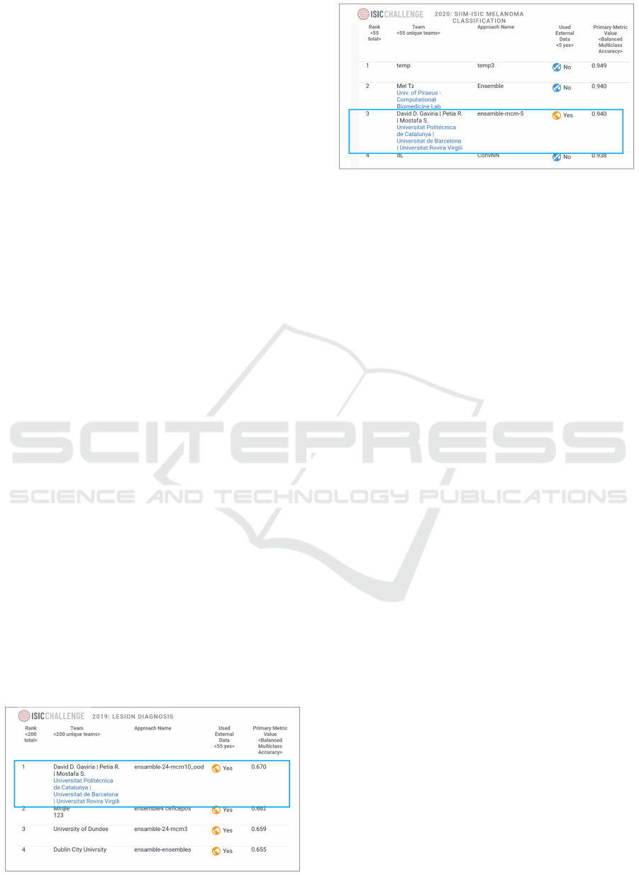
3.7.1 ISIC Submissions and Evaluation
We submitted our model to the ISIC Challenge sub-
mission system, which allows for automatic format
validation and scoring. Figure 9 and Table 8 resume
the results obtained from the unseen data for the 2019
Challenge and the 2020 ISIC challenge: (a) shows
the ROC Curve result for each individual class in the
2019 challenge, and (b) shows the melanoma predic-
tions results illustrated in the ROC Curve from the
ISIC 2020 dataset.
A brief look at Figure 9 ROC curve and AUC re-
veals that the ROC curve performs much worse with
the UNK class than with the other classes. Likewise
from Table 8, all classes have an AUC greater than
0.9, with the exception of the outlier class, which has
the lowest AUC of 0.595. Moreover, in the case of
melanoma, the AUC from table 8 shows a competent
score of 0.943 which motivated a submission in the
2020 ISIC challenge that assesses the malignant pre-
diction. The ROC Curve (b) in Figure 9 and the met-
rics results in Table 7 are the results of the submis-
sion to the 2020 ISIC live challenge. The 0.940 AUC
allowed the project to finish third in the 2020 ISIC
live challenge, confirming the proposal’s generaliza-
tion capabilities in a different test dataset.
Furthermore, only the regular CE was employed
in this experiment, which served to determine which
Figure 7: First place in 2019 ISIC live leaderboard.
Figure 8: Third place in 2020 ISIC live leaderboard.
augmentation strategy works best; the same behaviour
was observed by each one of the individual models.
Following the criteria from the melanoma ABCD rule
(Kasmi and Mokrani, 2016), our Adapted Augmen-
tation regime produced the best overall results, with
a greater Val BACC of 78.23% and 81.17% and an
overall score of 0.462 and 0.479 for the Inception-
Resnet-V2 and Swin-L-4, respectively. As a re-
sult, for all subsequent steps, this data augmentation
regime was used.
3.8 Study on the Modified Gram-OOD*
The purpose of this experiment was to assess the im-
provement that was yielded using the layer-wise cor-
relations compared to the activations of the Gram-
OOD* method from (Pacheco et al., 2020). Results
showed a significant improvement worth noting given
the reduced computational cost (10 epochs). Table 9
shows the feature maps extracted from the activation
and convolutional layers, respectively.
3.9 Study on the Loss Functions
The purpose of this experiment was to show the
thresholding approach to treat better the imbalanced
data compared to WCE. Moreover, since in many pa-
pers, Focal loss (FL) becomes well popular (Lin et al.,
2020), we compare our loss function to it too. Us-
ing two of the ensemble models; the Swin-L ViT and
Inception-Resnet-V2 representing CNNs; similar be-
haviour was observed on the rest of the models. Then,
table 10 compares the results of the assessed loss
functions to determine which approach among them
for dealing with imbalanced datasets in skin lesion
classification performs best.
The tests were carried out using the two kinds of
networks from the preceding section, both CNNs and
ViTs. These show that thresholding beats the other
two by a significant margin, ranging from 0.013 and
0.022 with the WCE to 0.005 and 0.009 with FL the
2019 challenge score. Thus, the thresholding strategy
Efficient Deep Learning Ensemble for Skin Lesion Classification
311
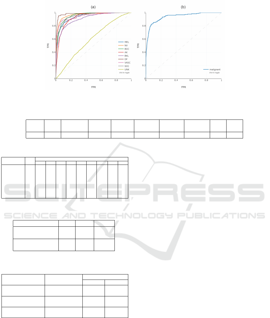
Figure 9: ROC curve for (a) the 0.670 BACC ensemble for the 2019 ISIC Challenge and (b) the melanoma with 0.940 AUC
for the 2020 ISIC Challenge.
Table 7: Ensemble melanoma metrics for top-3 in the 2020 ISIC live challenge.
Metric AUC
AUC
Sens >80%
Average
Precision
Accuracy Sensitivity Specificity
Dice
Coefficient
PPV NPV
MEL 0.940 0.899 0.544 0.982 0.284 0.999 0.426 0.852 0.983
Table 8: Ensemble metrics for top-1 in the 2019 ISIC.
Metrics Mean
Diagnosis Category
MEL NV BCC AK BKL DF VASC SCC UNK
AUC 0.908 0.943 0.965 0.955 0.928 0.911 0.983 0.947 0.949 0.595
AUC, Sens >80% 0.836 0.892 0.943 0.915 0.861 0.820 0.975 0.918 0.887 0.310
Average Precision 0.597 0.821 0.938 0.774 0.404 0.640 0.608 0.572 0.382 0.234
Accuracy 0.928 0.913 0.910 0.918 0.931 0.937 0.986 0.981 0.972 0.808
Sensitivity 0.589 0.658 0.797 0.788 0.610 0.490 0.733 0.653 0.573 0.00
Specificity 0.972 0.965 0.964 0.938 0.948 0.979 0.989 0.985 0.981 1.00
Dice Coefficient 0.538 0.719 0.851 0.716 0.474 0.572 0.559 0.482 0.471 0.00
PPV 0.630 0.791 0.913 0.655 0.388 0.688 0.452 0.382 0.400 1.00
NPV 0.948 0.933 0.908 0.967 0.978 0.953 0.997 0.995 0.991 0.808
Table 9: Comparison of the usage of convolutional layers
vs the activation functions as feature maps.
Method TNR AUC DTACC
Gram-OOD*
(Pacheco et al., 2020)
7.028 45.456 51.311
Modified Gram-OOD*
(Ours)
9.226 59.414 57.083
Table 10: Comparisom of different loss functions. Thresh-
olding was applied to the 2019 Score.
Imbalanced method Model
Metric
Val BACC 2019 Score
Weighted Cross Entropy
(Aurelio et al., 2019)
Inception-Resnet-V2 77.75% 0.502
Swin-L-4 80.63% 0.504
Focal Loss
(Lin et al., 2020)
Inception-Resnet-V2 78.03% 0.509
Swin-L-4 80.94 % 0.515
CE with thresholding
(Ours)
Inception-Resnet-V2 78.23% 0.514
Swin-L-4 81.17% 0.526
was adopted after the predictions, implying that the
CE had to be used as a loss function for training, and
thresholding was applied at the inference phase.
3.10 Discussion
When classifying skin lesions, especially in
melanoma appearance, it is important to con-
sider both the augmentation distortions and the
patient’s context (Strzelecki et al., 2021). When
viewed alongside the images, the metadata has
proven significant in every case. Moreover, an aug-
mentation scheme that alters a skin mole to resemble
a melanoma, especially when combined with elastic
asymmetric transformations or grid distortions, may
seriously hinder the NN learning capabilities.
4 CONCLUSIONS
Based on the diagnosis of skin lesions and recent pub-
lications, two open live challenges—ISIC 2019 and
ISIC 2020— were used to study the classification of
dermatological images and validate the overall perfor-
mance of the DL solutions. Our study proves that no
single model, nor ViTs neither CNNs could achieve a
higher standing in both the 2019 and 2020 ISIC live
challenges. Our ensemble of ViTs and CNNs was
able to provide a huge diversity, necessary to achieve
top-1 for the ISIC 2019 live challenge with a BACC
of 0.670, and top-3 for melanoma classification in the
ISIC-2020 live challenge with an AUC score of 0.940.
Additionally, we used the same target prediction
for the malignant melanoma, indicating strong gen-
eralization potential to close the gap in considering
deep learning techniques as a reliable source for an
early diagnosis. Although the data used here mixed
dermoscopy and clinical images, further research is
required to assess the behavior of a DL solution with
a bulk of clinical images in the test set. Despite im-
provements made in the topic of outliers, both for the
data-driven approach and from the modified Gram-
VISAPP 2023 - 18th International Conference on Computer Vision Theory and Applications
312

OOD* adaptation, the OOD samples present in the
2019 ISIC remain an open challenge and further re-
search on the topic is required to improve OOD de-
tection for both CNNs and ViTs.
The ideal use for this technology would be a mo-
bile app or online diagnostic tool that offers practi-
cal, prompt advise of whether a patient should con-
sult a doctor about a worrisome lesion. To get close
to that, a demo created along with further details may
be found at: https://skin-lesion-diagnosis.web.app/.
ACKNOWLEDGEMENTS
This work was partially funded from the European
Union’s Horizon 2020 MUSAE project, Erasmus+
project RoboSteam, Acci
´
o Nuclis project DeepSens,
and CERCA Programme / Generalitat de Catalunya.
B. Nagarajan acknowledges the support of FPI Be-
cas, MICINN, Spain. We acknowledge the support of
NVIDIA Corporation with the donation of the Titan
Xp GPUs.
REFERENCES
ACS, A. C. S. (2022). Key statistics for melanoma skin can-
cer. https://www.cancer.org/cancer/melanoma-skin-
cancer/about/key-statistics.html. Accessed: 2022-08-
30.
Ali, D. A.-R., Li, J., and O’Shea, S. J. (2020). Towards
the automatic detection of skin lesion shape asymme-
try, color variegation and diameter in dermoscopic im-
ages. PLoS ONE, 15.
Archive, I. (2019). Evaluation score. https://challenge.isic-
archive.com/landing/2019/. Accessed: 2022-06-30.
Aurelio, Y. S., de Almeida, G. M., de Castro, C. L., and
de P
´
adua Braga, A. (2019). Learning from imbalanced
data sets with weighted cross-entropy function. Neu-
ral Processing Letters, 50:1937–1949.
Bao, H., Dong, L., and Wei, F. (2022). Beit:
Bert pre-training of image transformers. ArXiv,
abs/2106.08254.
Belilovsky, E., Eickenberg, M., and Oyallon, E. (2019).
Greedy layerwise learning can scale to imagenet.
ArXiv, abs/1812.11446.
Buda, M., Maki, A., and Mazurowski, M. A. (2018). A
systematic study of the class imbalance problem in
convolutional neural networks. Neural networks : the
official journal of the International Neural Network
Society, 106:249–259.
Chang, W.-Y., Huang, A., Yang, C.-Y., Lee, C.-H., Chen,
Y.-C., Wu, T.-Y., and Chen, G.-S. (2013). Computer-
aided diagnosis of skin lesions using conventional dig-
ital photography: A reliability and feasibility study.
PLoS ONE, 8.
Chen, J., Chen, J., Zhou, Z., Li, B., Yuille, A. L., and Lu,
Y. (2021). Mt-transunet: Mediating multi-task tokens
in transformers for skin lesion segmentation and clas-
sification. ArXiv, abs/2112.01767.
Chen, T., Kornblith, S., Norouzi, M., and Hinton, G. E.
(2020). A simple framework for contrastive learning
of visual representations. ArXiv, abs/2002.05709.
Combalia, M., Codella, N. C. F., Rotemberg, V. M., Helba,
B., Vilaplana, V., Reiter, O., Halpern, A. C., Puig, S.,
and Malvehy, J. (2019). Bcn20000: Dermoscopic le-
sions in the wild. ArXiv, abs/1908.02288.
Cubuk, E. D., Zoph, B., Man
´
e, D., Vasudevan, V., and Le,
Q. V. (2019). Autoaugment: Learning augmentation
strategies from data. 2019 IEEE/CVF CVPR, pages
113–123.
Cubuk, E. D., Zoph, B., Shlens, J., and Le, Q. V. (2020).
Randaugment: Practical automated data augmenta-
tion with a reduced search space. 2020 IEEE/CVF
CVPRW, pages 3008–3017.
Devries, T. and Taylor, G. W. (2017). Improved regular-
ization of convolutional neural networks with cutout.
ArXiv, abs/1708.04552.
Dosovitskiy, A., Beyer, L., Kolesnikov, A., Weissenborn,
D., Zhai, X., Unterthiner, T., Dehghani, M., Min-
derer, M., Heigold, G., Gelly, S., Uszkoreit, J., and
Houlsby, N. (2021). An image is worth 16x16 words:
Transformers for image recognition at scale. ArXiv,
abs/2010.11929.
Forsea, A. M. (2020). Melanoma epidemiology and early
detection in europe: Diversity and disparities. Derma-
tology practical & conceptual, 10 3:e2020033.
Gessert, N., Nielsen, M., Shaikh, M., Werner, R., and
Schlaefer, A. (2020). Skin lesion classification using
ensembles of multi-resolution efficientnets with meta
data. MethodsX, 7.
Giotis, I., Molders, N., Land, S., Biehl, M., Jonkman,
M. F., and Petkov, N. (2015). Med-node: A
computer-assisted melanoma diagnosis system us-
ing non-dermoscopic images. Expert Syst. Appl.,
42:6578–6585.
Ha, Q., Liu, B., and Liu, F. (2020). Identifying melanoma
images using efficientnet ensemble: Winning solution
to the siim-isic melanoma classification challenge.
ArXiv, abs/2010.05351.
Hendrycks, D., Mu, N., Cubuk, E. D., Zoph, B., Gilmer, J.,
and Lakshminarayanan, B. (2020). Augmix: A sim-
ple data processing method to improve robustness and
uncertainty. ArXiv, abs/1912.02781.
Heo, B., Chun, S., Oh, S. J., Han, D., Yun, S., Kim, G.,
Uh, Y., and Ha, J.-W. (2021). Adamp: Slowing down
the slowdown for momentum optimizers on scale-
invariant weights. arXiv: Learning.
Kasmi, R. and Mokrani, K. (2016). Classification of malig-
nant melanoma and benign skin lesions: implemen-
tation of automatic abcd rule. IET Image Process.,
10:448–455.
Liang, S., Li, Y., and Srikant, R. (2018). Enhancing the reli-
ability of out-of-distribution image detection in neural
networks. arXiv: Learning.
Efficient Deep Learning Ensemble for Skin Lesion Classification
313

Lin, T.-Y., Goyal, P., Girshick, R. B., He, K., and Doll
´
ar, P.
(2020). Focal loss for dense object detection. IEEE
Transactions on Pattern Analysis and Machine Intel-
ligence, 42:318–327.
Liu, Z., Hu, H., Lin, Y., Yao, Z., Xie, Z., Wei, Y., Ning,
J., Cao, Y., Zhang, Z., Dong, L., Wei, F., and Guo,
B. (2022a). Swin transformer v2: Scaling up capac-
ity and resolution. IEEE/CVF CVPR, pages 11999–
12009.
Liu, Z., Lin, Y., Cao, Y., Hu, H., Wei, Y., Zhang, Z., Lin,
S., and Guo, B. (2021). Swin transformer: Hierarchi-
cal vision transformer using shifted windows. 2021
IEEE/CVF ICCV, pages 9992–10002.
Liu, Z., Mao, H., Wu, C., Feichtenhofer, C., Darrell, T.,
and Xie, S. (2022b). A convnet for the 2020s. pages
11976–11986.
Nikita Kozodoi, Gilberto Titericz, H. G. (2020). 11th
place solution writeup. https://www.kaggle.
com/competitions/siim-isic-melanoma-classification/
discussion/175624. Accessed: 2022-04-30.
Pacheco, A. G. C., Sastry, C. S., Trappenberg, T. P., Oore,
S., and Krohling, R. A. (2020). On out-of-distribution
detection algorithms with deep neural skin cancer
classifiers. IEEE/CVF CVPRW, pages 3152–3161.
Potdar, K., Pardawala, T. S., and Pai, C. D. (2017). A com-
parative study of categorical variable encoding tech-
niques for neural network classifiers. International
Journal of Computer Applications, 175:7–9.
Richard, M. D. and Lippmann, R. (1991). Neural network
classifiers estimate bayesian a posteriori probabilities.
Neural Computation, 3:461–483.
Rotemberg, V. M., Kurtansky, N. R., Betz-Stablein, B., Caf-
fery, L. J., Chousakos, E., Codella, N. C. F., Combalia,
M., Dusza, S. W., Guitera, P., Gutman, D., Halpern,
A. C., Kittler, H., K
¨
ose, K., Langer, S. G., Liopryis,
K., Malvehy, J., Musthaq, S., Nanda, J., Reiter, O.,
Shih, G., Stratigos, A. J., Tschandl, P., Weber, J., and
Soyer, H. P. (2021). A patient-centric dataset of im-
ages and metadata for identifying melanomas using
clinical context. Scientific Data, 8.
Russakovsky, O., Deng, J., Su, H., Krause, J., Satheesh, S.,
Ma, S., Huang, Z., Karpathy, A., Khosla, A., Bern-
stein, M. S., Berg, A. C., and Fei-Fei, L. (2015). Im-
agenet large scale visual recognition challenge. Inter-
national Journal of Computer Vision, 115:211–252.
Sarker, M. M. K., Moreno-Garc
´
ıa, C. F., Ren, J., and
Elyan, E. (2022). Transslc: Skin lesion classifica-
tion in dermatoscopic images using transformers. In
Annual Conference on Medical Image Understanding
and Analysis, pages 651–660. Springer.
Sastry, C. S. and Oore, S. (2019). Detecting out-of-
distribution examples with in-distribution examples
and gram matrices. ArXiv, abs/1912.12510.
Shanmugam, D., Blalock, D. W., Balakrishnan, G., and
Guttag, J. V. (2020). When and why test-time aug-
mentation works. ArXiv, abs/2011.11156.
Smith, L. N. (2018). A disciplined approach to neu-
ral network hyper-parameters: Part 1 - learning rate,
batch size, momentum, and weight decay. ArXiv,
abs/1803.09820.
Smith, L. N. and Topin, N. (2019). Super-convergence: very
fast training of neural networks using large learning
rates. In Defense + Commercial Sensing.
Steppan, J. and Hanke, S. (2021). Analysis of skin lesion
images with deep learning. ArXiv, abs/2101.03814.
Strzelecki, M., Strakowska, M., Kozłowski, M., Urba
´
nczyk,
T., Wielowieyska-Szybi
´
nska, D., and Kociolek, M.
(2021). Skin lesion detection algorithms in whole
body images. Sensors (Basel, Switzerland), 21.
Sun, X., Yang, J., Sun, M., and Wang, K. (2016). A
benchmark for automatic visual classification of clin-
ical skin disease images. In ECCV.
Szegedy, C., Ioffe, S., Vanhoucke, V., and Alemi, A. A.
(2017). Inception-v4, inception-resnet and the impact
of residual connections on learning. In AAAI.
Tan, M. and Le, Q. V. (2019). Efficientnet: Rethink-
ing model scaling for convolutional neural networks.
ArXiv, abs/1905.11946.
Touvron, H., Cord, M., Douze, M., Massa, F., Sablayrolles,
A., and J’egou, H. (2021a). Training data-efficient im-
age transformers & distillation through attention. In
ICML.
Touvron, H., Cord, M., Sablayrolles, A., Synnaeve, G., and
J’egou, H. (2021b). Going deeper with image trans-
formers. 2021 IEEE/CVF ICCV, pages 32–42.
Tschandl, P., Rosendahl, C., and Kittler, H. (2018). The
ham10000 dataset, a large collection of multi-source
dermatoscopic images of common pigmented skin le-
sions. Scientific Data, 5.
Vaswani, A., Shazeer, N. M., Parmar, N., Uszkoreit, J.,
Jones, L., Gomez, A. N., Kaiser, L., and Polosukhin,
I. (2017). Attention is all you need. In NIPS.
Walter, F. M., Prevost, A. T., Vasconcelos, J. C., Hall, P.,
Burrows, N. P., Morris, H. C., Kinmonth, A. L., and
Emery, J. D. (2013). Using the 7-point checklist as
a diagnostic aid for pigmented skin lesions in general
practice: a diagnostic validation study. The British
journal of general practice : the journal of the Royal
College of General Practitioners, 63 610:e345–53.
WHO, W. H. O. (2017). Radiation: Ultraviolet (uv)
radiation and skin cancer. https://www.who.int/news-
room/questions-and-answers/item/radiation-
ultraviolet-(uv)-radiation-and-skin-cancer. Accessed:
2022-06-30.
Xie, Q., Hovy, E. H., Luong, M.-T., and Le, Q. V. (2020).
Self-training with noisy student improves imagenet
classification. IEEE/CVF CVPR, pages 10684–10695.
Xie, S., Girshick, R. B., Doll
´
ar, P., Tu, Z., and He, K.
(2017). Aggregated residual transformations for deep
neural networks. IEEE CVPR, pages 5987–5995.
Yalniz, I. Z., J
´
egou, H., Chen, K., Paluri, M., and Mahajan,
D. K. (2019). Billion-scale semi-supervised learning
for image classification. ArXiv, abs/1905.00546.
Yuan, L., Hou, Q., Jiang, Z., Feng, J., and Yan, S. (2022).
Volo: Vision outlooker for visual recognition. IEEE
Trans. PAMI, PP.
VISAPP 2023 - 18th International Conference on Computer Vision Theory and Applications
314
