Redundancy and Novelty Between ECG Leads Based on Linear

Correlation

Utkars Jain

1 a

, Adam A. Butchy

1 b

, Michael T. Leasure

1 c

, Veronica A. Covalesky

2,3

Daniel McCormick

2,3

and Gary S. Mintz

4 d

Heart Input Output Inc., 128 N. Craig Street, Suite 406, Pittsburgh, U.S.A.

Cardiology Consultants of Philadelphia, Philadelphia, Pennsylvania, U.S.A.

Jefferson University Hospital, Philadelphia, Pennsylvania, U.S.A.

The Cardiovascular Research Foundation, New York, New York, U.S.A.

Keywords:

Statistics, ECGs, Cardiac, Correlation.

Abstract:

ECGs are a common diagnostic method for diagnosing cardiac pathologies. In this study, the Pearson correla-

tion coefﬁcient is used to examine the latent linear correlations between the leads of a standard 12-lead ECG.

We utilize both the original ECG signals from the PTB-XL database and the reconstructed signal generated

by a deep learning model, ECGio. We ﬁnd that leads III, aVL, V1, and V2 are, on average, the leads with the

most unique information due to their low correlation with other leads.

1 INTRODUCTION

Clinicians use a range of diagnostic techniques to de-

tect and identify heart and circulatory problems. Elec-

trocardiograms (ECGs), Troponin biomarker testing,

coronary computed tomography angiograms (CC-

TAs), magnetic resonance imaging (MRI), positron

emission tomography (PET), fractional ﬂow reserve

(FFR), and coronary angiography are the most fre-

quently performed. These tests search for structural,

vascular, or electrical abnormalities in the cardiovas-

cular system of a patient (DeLaney et al., 2017). This

paper focuses on the noninvasive, ubiquitous, and in-

expensive electrocardiogram (ECG).

Invented in the 1870s, the ECG is a simple yet

effective monitoring device for the heart’s electrical

beats and rhythms (AlGhatrif and Lindsay, 2012).

The standard 12-lead ECG consists of nine electrodes

connected to speciﬁed locations on the patient’s body

and one electrode serving as an electrical ground. The

ECG machine then measures the voltage difference

between speciﬁc electrodes on the body to generate

waveforms that represent the building, release, and

refractory phases of the heart’s electrical cycle (Yang

https://orcid.org/0000-0002-1800-0768

https://orcid.org/0000-0002-0096-0031

https://orcid.org/0000-0002-1488-712X

https://orcid.org/0000-0003-3296-8705

et al., 2015). A bipolar electrode is created by sub-

tracting voltage of the ground electrode from the volt-

age of another electrode. Unipolar have a single pos-

itive electrode and utilize a combination of the other

electrodes to serve as the negative electrode (Derganc

and Gomi

cek, 2021). ECGs can be conﬁgured in a

variety of ways - all conﬁgurations differ based on the

placement, location, and number of leads.

The 12-lead resting ECG is the most common

(Harris, 2016) but several other types exist. Holter

ECGs may contain 2, 3, 6, or even 12 leads and are

used for continuous patient monitoring (DiMarco and

Philbrick, 1990). There exist more complicated de-

vices that use far more than 12 leads, and may even

take a full-body reading with a vest-like device (Wang

et al., 2019). Recent advancements in personal elec-

tronics have enabled the integration of 1-lead ECG

devices into smartwatches (Samol et al., 2019). In

table 1, we have a description of the 12 leads of the

normal resting ECG system.

In this paper, we analyze the linear correlation be-

tween ECG leads as a measure of information redun-

dancy using the standard 12-lead ECG and its asso-

ciated leads. We determine if there are speciﬁc leads

that carry less redundant information when compared

to others. Prior research investigated the use of AI to

more thoroughly analyze ECGs and how to use ECGs

with fewer than 12 leads to improve ECG signals (Jain

Jain, U., Butchy, A., Leasure, M., Covalesky, V., McCormick, D. and Mintz, G.

Redundancy and Novelty Between ECG Leads Based on Linear Correlation.

DOI: 10.5220/0011815700003414

In Proceedings of the 16th International Joint Conference on Biomedical Engineering Systems and Technologies (BIOSTEC 2023) - Volume 4: BIOSIGNALS, pages 359-365

ISBN: 978-989-758-631-6; ISSN: 2184-4305

 2023 by SCITEPRESS – Science and Technology Publications, Lda. Under CC license (CC BY-NC-ND 4.0)

359

Table 1: The 12 leads, the location of the positive and neg-

ative electrodes, and which heart surface they are thought

to represent. “N” refers to neutral or electric ground. +

Location refers to the positive electrode location, while -

Location refers to the negative electrode location.

Lead + Location - Location Surface

I Left Arm Right Arm Lateral

II Left Leg Right Arm Inferior

III Left Leg Left Arm Inferior

aVR Right Arm N None

aVL Left Arm N Lateral

aVF Left Leg N Inferior

Right side of sternum,

4th intercostal space

N Septum

Left side of sternum,

4th intercostal space

N Septum

V3 Between V2 & V4 N Anterior

Left midclavicular line,

5th intercostal place

N Anterior

V5 Left anterior axillary line N Lateral

V6 Left midaxillary line N Lateral

et al., 2022), we will use the methods of reconstruc-

tion to conclude if lead relationships are carried over.

The correlation between distinct sets of leads will de-

termine the redundancy and novelty of leads. Corre-

lation will be deﬁned by the Pearson correlation coef-

ﬁcient, also known as Pearson’s r.

2 RELATED WORKS

There have been other works that look into the cal-

culation or use of inter-lead relationships or corre-

lations between the lead of an ECG signals. Zhang

et. al set out to investigate a possible reason as to

why deep learning networks generalize pretty well in

the detection of left bundle brach block (LBBB) even

with small data sizes. They discovered that the cor-

relation between lead V1 and other leads was close

to 0, and a set correlation matrix can be indicative of

LBBB (Zhang et al., 2022). Jekova et. al used inter-

lead relationships in order to identify misplaced leads

or cable reversals resulting in a ﬂipped signal. They

were able to build a robust algorithm that was able to

identify cable reversals based on inter-lead relation-

ships (Jekova et al., 2016).

3 METHODS

The Pearson correlation coefﬁcient quantiﬁes the lin-

ear correlation between two sets of data, providing a

measure of how closely a linear model would ﬁt to

the data sets. An r value closer to 1 indicates a strong

positive correlation while a value closer to -1 indi-

cates a strong negative correlation. An r value of 0

indicates no correlation between the two datasets. A

generally accepted interpretation of the correlation is

that if there is a strong positive or negative correla-

tion that there is a redundancy in data (Schober et al.,

2018). (I.e one dataset is a scaled version of the other.)

If there is no correlation then there is novel informa-

tion contained between the two different datasets. A

visual example of the pearson correlation coefﬁcient

based on scatter plot data is seen in ﬁgure 1. A vi-

sual example using ECG data from patient ﬁle 06275

is shown in 2.

The Pearson correlation coefﬁcient, or r is deﬁned

as:

r(y, ˆy) =

E[(y − µ

)( ˆy −µ

ˆy

)]

ˆy

(1)

Non-linear correlation cannot be measured by the

Pearson correlation coefﬁcient. This indicates that

something may be highly uncorrelated in the linear

sense but correlated in the nonlinear sense. To main-

tain a solid basis for interpretation, nonlinear correla-

tions between leads fall outside the scope of this anal-

ysis.

We used 250 randomly selected patients from

PTB-XL, a large public electrocardiography dataset,

to conduct this study (Wagner et al., 2020). We chose

250 patients because this population served as the test

set for our reconstruction experiments and will now

serve as a good baseline to compare original signals

and reconstructed signals. These were a random sam-

ple of healthy and pathological ECGs. One in which

the original signal is present and one in which the sig-

nal has been reconstructed by a deep learning model

called ECGio (Leasure et al., 2021). In a previous

paper, the performance of ECGio in recreating ECGs

using the same 250 patients was demonstrated (Jain

et al., 2022). Maintaining patient consistency will

prevent bias and preserve the same testing set. Since

the deep learning model is expected to correct awry

signals, we will determine whether these correlations

are inherent to the ECGs or a result of noise.

The ECG signal input that was used to analyze

correlation was standardized. Each ECG signal was

clipped to represent 10 seconds of ECG time, with

the form NxM, where M was the number of leads

and N was the number of samples. Given that each

signal lasted just 10 seconds, N was also equal to

10 times the sampling rate. We resampled the sig-

nal using Fast Fourier Transform (FFT) to reduce the

sampling rate to 100Hz. This was done through the

scipy.signal.resample method

which assumes a pe-

riodic signal and transforms the signals to the fre-

docs.scipy.org/doc/scipy/reference/generated/scipy.sig

nal.resample.html

BIOSIGNALS 2023 - 16th International Conference on Bio-inspired Systems and Signal Processing

360

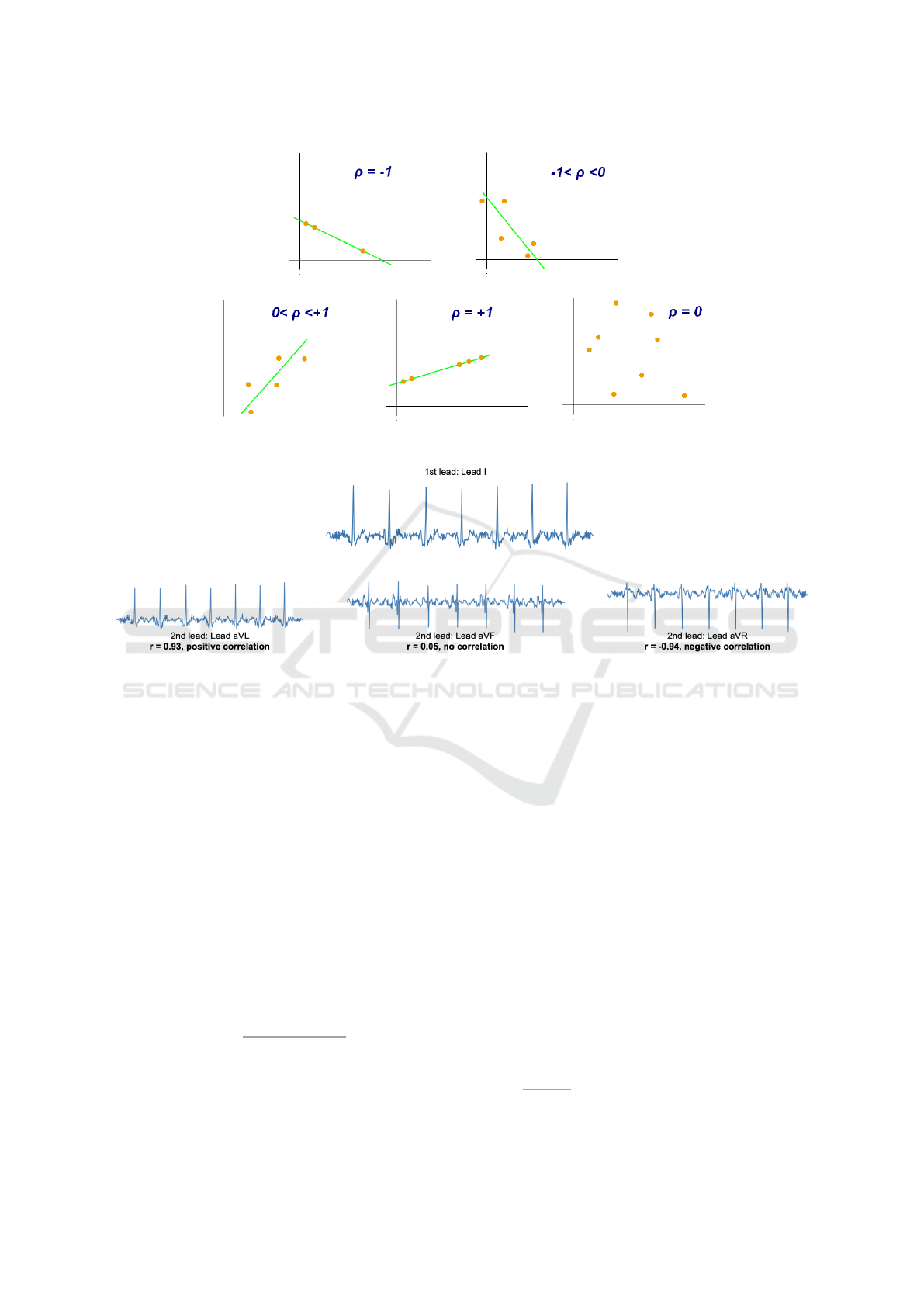
Figure 1: Visual example of the Pearson correlation coefﬁcient based on scatter plot data. Illustration was provided by user

Kiatdd from Wikimedia Commons, under the Creative Commons Attribution-Share Alike 3.0 Unported license.

Figure 2: Visual example of the Pearson correlation coefﬁcient based on ECG data. The initial comparative lead is lead I, and

it is compared to the unipolar leads. lead I is shown to have a strong positive correlation to lead aVR, no correlation with lead

aVF, and a strong negative correlation with lead aVL.

quency domain and removes unnecessary parts of the

domain and transforms it back. We employed a Band-

pass Butterworth ﬁlter with a passband beginning at

2Hz and ending at 40Hz to ensure that only informa-

tion within this band of frequencies was kept while

all others were discarded. Frequencies below 2Hz are

where breathing and muscle noise may interfere with

the signal (Li et al., 2017) and 40Hz is shown to be an

adequate cutoff (Ricciardi et al., 2016).

The databased ECG signals were obtained with

non-standardized minimum and maximum values in

millivolts (mV). Conforming to best practices in ma-

chine learning (Jo, 2019), we scaled each ten-second

ECG segment to values between [-1, +1] using equa-

tion 2, as is customary in deep learning to normalize

input signals:

f (x) = 2

x − min(x)

max(x) − min(x)

− 1 (2)

If x represented an ECG array in millivolts (mV),

max(x) represented the largest value along x, and

min(x) represented the minimum value along x. All

null values were transformed into zeros. Each signal

was eventually detrended to the point where the iso-

electric sections of the ECG were equal to zero.

The 12-lead standardized data served as the ba-

sis for calculating performance metrics. We did not

employ raw voltage difference values as the reference

to avoid a huge potential variance in the presence of

muscle, movement, or electric noise creating signal-

to-signal deviations. Mathematically, standardized

signals would provide a more equitable comparison,

whereas a direct comparison of performance indica-

tors between our outcomes and those of others may

not be prudent.

There are two primary methods to calculate the

Pearson correlation coefﬁcient. One is that we loop

over every combination of the two leads in the ECG

(e.g. lead I against itself, lead I against lead II, etc.)

and apply the formula. This method would require

us to go through every combination for every ECG.

Meaning that in total there would be 66 calculations





12!

2!(12−2)!

for a 12-lead ECG. This is not an in-

surmountable number of calculations, but in the case

Redundancy and Novelty Between ECG Leads Based on Linear Correlation

361

for ECGs with many more leads, we would like a

more scalable solution. The second method is a vec-

torized approach, i.e. creating a correlation matrix, in

which there is a series of vector and matrix based cal-

culations, resulting in many less overall calculations.

A correlation matrix was established for each of

the 250 patients original and reconstructed ECGs.

Each of these matrices were layered to generate a

three dimensional tensor (size of 250x12x12). We did

three alternative sets of operations of the ﬁrst axis of

this tensor: obtaining the mean, maximum, and mini-

mum. After these processes were ﬁnished, there were

6 separate correlation matrices. A mean, maximum,

and minimum correlation matrix for the original and

reconstructed signals. The reason why maximum and

minimum were selected was because we were under

the assumption that there would high levels of corre-

lations between any 2 leads for at least one patient -

we were looking to determine whether there were any

combinations in which their extremes broke the trend.

Algorithm 1: Algorithm for calculating correlation matrix.

Ensure: X− > Mx N ▷ X is the ECG matrix

∗

= X − µ(X) ▷ Subtract X by mean value in lead

axis

∗∗

= X

∗

· X

∗

▷ Matrix multiplication of X

∗

Z = σ(

diag(X

∗∗

)) ▷ Scaling based on

covariance

R =

∗∗

▷ Correlation Matrix

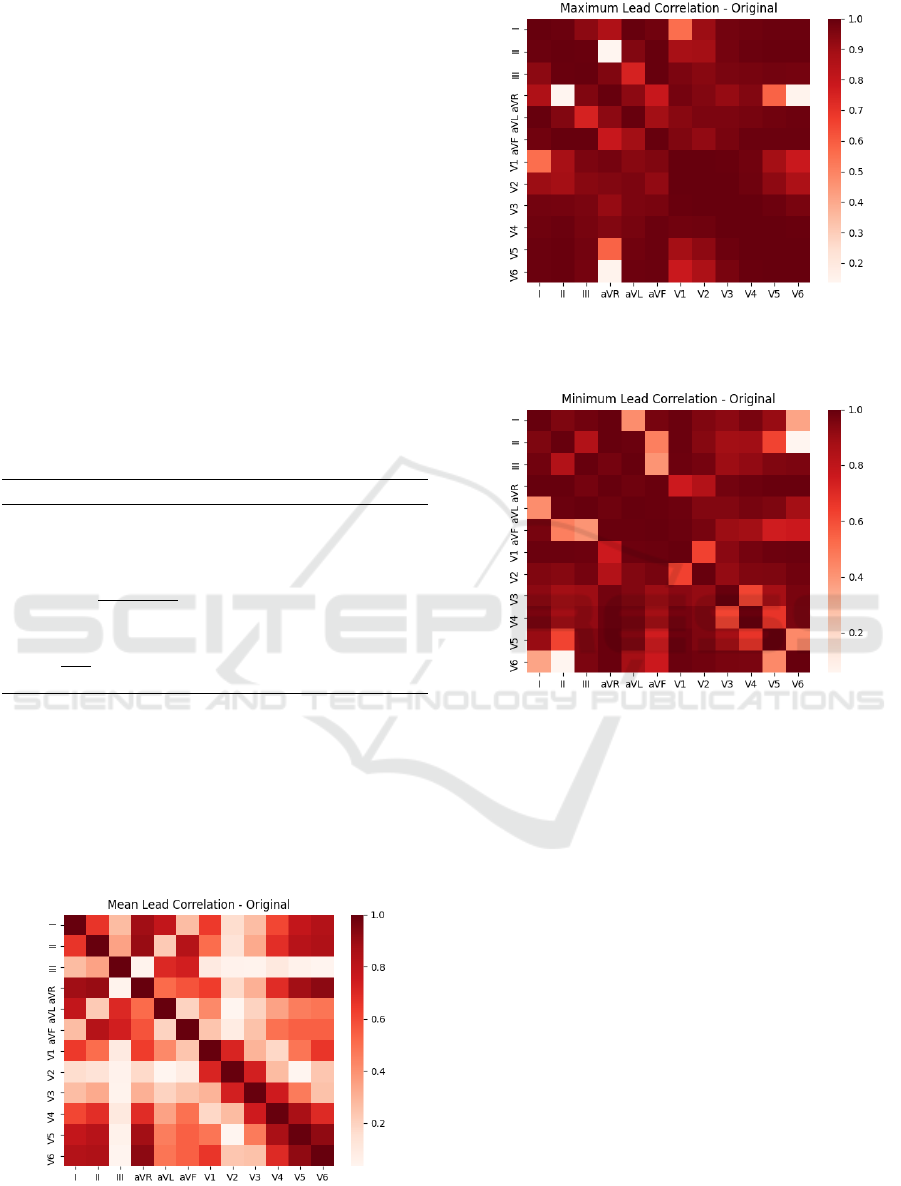
4 RESULTS

The results of our two experiments are shown. In

ﬁgures 3, 4, 5, 6, 7, and 8 we have heatmaps show-

ing the cross correlation between all of the standard

ECG leads for the original patient ECGs and the re-

Figure 3: The ﬁgure below shows a heatmap of the mean

correlation matrix over the population of patients examined

with the original signals.

Figure 4: The ﬁgure below shows a heatmap of the maxi-

mum correlation matrix over the population of patients ex-

amined with the original signals.

Figure 5: The ﬁgure below shows a heatmap of the mini-

mum correlation matrix over the population of patients ex-

amined with the original signals.

constructed ones. Those that are more correlated have

a darker color while the ones that are more uncorre-

lated are a lighter color. In tables 2 and 3 we see the

mean, maximum, and minimum values for each lead

when analyzing their correlations with other leads for

the original ECGs and their reconstructions. In ta-

ble 4 we examine the differences between the maxi-

mum and minimum correlation matrices for the orig-

inal ECGs and their reconstructions.

5 DISCUSSION

The Pearson correlation coefﬁcient is a prevalent ap-

proach for analyzing the linear relationship between

continuous variables (Benesty et al., 2009). It can

provide a great deal of broad information about vari-

ables with a single value. However, it should be high-

lighted that this is not a foolproof method for deter-

mining the correlation between signals or variables.

BIOSIGNALS 2023 - 16th International Conference on Bio-inspired Systems and Signal Processing

362

Figure 6: The ﬁgure below shows a heatmap of the mean

correlation matrix over the population of patients examined

with the reconstructed signals.

Figure 7: The ﬁgure above shows a heatmap of the maxi-

mum correlation matrix over the population of patients ex-

amined with the reconstructed signals.

Figure 8: The ﬁgure above shows a heatmap of the mini-

mum correlation matrix over the population of patients ex-

amined with the reconstructed signals.

We are simply evaluating the linear correlation of the

signal. Essentially, we wish to determine whether

the signals ﬂuctuate synchronously. Do they rise or

Table 2: The table below shows the mean, maximum, and

minimum correlations per lead when compared to other

leads (sans the lead itself), when analyzing the mean cor-

relation matrix from the 250 patients. Leads that shown to

have signiﬁcant degrees of uncorrelation are denoted with

an *.

Lead Mean r Max r Min r

I 0.205 0.832 -0.645

II 0.290 0.846 -0.507

III* 0.033 0.738 -0.272

aVR -0.447 0.636 -0.903

aVL* 0.057 0.787 -0.516

aVF 0.233 0.828 -0.245

V1* -0.128 0.714 -0.645

V2* 0.104 0.734 -0.163

V3 0.299 0.749 0.047

V4 0.359 0.862 -0.183

V5 0.319 0.920 -0.483

V6 0.254 0.920 -0.658

Table 3: The table below shows the mean, maximum, and

minimum correlations per lead when compared to other

leads (sans the lead itself), when analyzing the mean cor-

relation matrix from reconstructions of the 250 patients.

Leads that shown to have signiﬁcant degrees of uncorrela-

tion are denoted with an *.

Lead Mean r Max r Min r

I 0.220 0.859 -0.863

II 0.291 0.867 -0.884

III* 0.050 0.687 -0.620

aVR -0.450 0.649 -0.937

aVL* 0.065 0.732 -0.620

aVF 0.241 0.804 -0.579

V1* -0.152 0.710 -0.707

V2* 0.102 0.739 -0.250

V3 0.299 0.749 -0.326

V4 0.362 0.850 -0.712

V5 0.318 0.930 -0.899

V6 0.256 0.930 -0.937

decrease simultaneously? All other connections are

considered uncorrelated.

The Pearson correlation coefﬁcient does not ac-

count for the magnitude of differences and is highly

prone to outliers (Kim et al., 2015). For instance,

there may be a large number of points centered about

the origin and only a few along the x-axis. The Pear-

son correlation coefﬁcient will depend heavily on how

these few points behave. We attempted to preprocess

and standardize the data in order to make fair com-

parisons, but this does not ensure the elimination of

outliers.

In a typical 12-lead ECG setup there are 2-3 limb

leads, leads attached to the arms or legs, and pre-

cordial (or chest) leads, leads attached to the chest.

Redundancy and Novelty Between ECG Leads Based on Linear Correlation

363

Table 4: The table below shows the mean correlations per

lead when compared to other leads (sans the lead itself),

when analyzing the maximum and minimum correlation

matrices from both the original 250 patients and the recon-

structed ECGs.

Lead

Original

Min

Original

Max

Reconstructed

Min

Reconstructed

Max

I -0.857 0.926 -0.904 0.940

II -0.786 0.866 -0.816 0.901

III -0.897 0.948 -0.940 0.961

aVR -0.954 0.695 -0.969 0.710

aVL -0.917 0.939 -0.957 0.964

aVF -0.827 0.954 -0.859 0.964

V1 -0.929 0.903 -0.950 0.921

V2 -0.913 0.942 -0.924 0.960

V3 -0.895 0.974 -0.929 0.982

V4 -0.890 0.984 -0.937 0.985

V5 -0.828 0.939 -0.810 0.932

V6 -0.759 0.856 -0.773 0.855

The idea behind this setup is that limb leads provided

information about the electrical propagation along a

longer axis, while the chest leads provide information

that is closer to the heart (Dower et al., 1990). These

2 sets of information combined can lead to a more

holistic interpretation of the heart’s electrical activity.

The unipolar leads (aVL, aVF, aVR) are constructed

through a linear combination of the limb leads (Ma-

dias, 2008).

Lead III, which can occasionally be created from

leads I and II (lead III = lead II - lead I), appears to

be linearly uncorrelated with the mean of the original

patients. This is unexpected because it can be viewed

as a linear combination of leads I and II, yet there ap-

pears to be novel information in terms of correlation.

Because lead I, II, and III are based upon a trigono-

metric relationship, it’s possible that correlations be-

tween them are not fully captured looking at linear

relationships.

As seen in ﬁgures 3 and 6, the precordial leads, on

average, seemed to be relatively uncorrelated when

compared against the limb leads and the unipolar

leads. This would be in line with the thought process

that precordial leads are assessing different surfaces

of the heart, and thus yield different information.

An intriguing phenomena in the maximum and

minimum correlation of the original patients is that

there are several correlations between leads that are

close to +1 or -1. Even more unexpectedly, in our

dataset, some correlations remained near 0 even when

searching for the maximum or minimum value.

For instance, when searching for the maximal cor-

relations, V6 has a correlation value of -0.14 when

compared to aVR. This implies that, across the tested

population, there was little correlation between these

two leads, but V6 showed the strong correlation with

other unipolar leads. aVR is a linear combination of

leads I and II, but its combination may contain infor-

mation that differs signiﬁcantly from what was pre-

viously believed (Williamson et al., 2006). Another

similar case is between lead V6 and lead II, when

looking for the minimum correlation case the value is

-0.05. There may be an obvious explanation for unex-

pectedly signiﬁcant correlations, namely that the lead

was improperly positioned and hence captured signals

that heavily overlapped with the domain of another

lead for a particular ECG of a patient.

According to tables 2 and 3, leads III, aVL, V1,

and V2 had the lowest average correlation. Using a

threshold of 0.2, it was possible to determine which

leads were uncorrelated. These leads offer informa-

tion regarding the inferior, lateral, and septal sur-

faces of the heart (both lead V1, V2 offer informa-

tion about the septal surface), which represent three

of the heart’s four primary surfaces (lateral, inferior,

septum, and anterior). Possible interpretation: these

leads contain the most novel information regarding

these surfaces. In the future, it may be necessary to

determine if the novel information contained in these

leads facilitates better levels of ECG reconstruction

performance.

Our analysis uncovered the intriguing conclusion

that the ECG reconstruction data closely resemble the

original data. The goal of comparing the original cor-

relation to that of the reconstruction was to determine

if these correlations were intrinsic to the ECG itself

and not the result of noise or lead placement, which

the deep learning model is designed to correct.

Based on the similar levels of correlation, it may

be concluded that a 12-lead ECG contains a latent

structure that is known during model training. It is

feasible that the model is just learning to match the

output as closely as possible, without learning any in-

trinsic structure. In the future, it may be necessary

to determine whether or not the model attempts to

comprehend the ECG’s underlying structure when re-

building the input.

6 CONCLUSION

In this study, we examined the average lead corre-

lations of 250 patient ECG signals from the phys-

ionet PTB-XL database. We studied the original sig-

nals while they were being normalized and when they

were being reconstructed using a novel deep learning

technique. The mean, maximum, and minimum cor-

relations between the leads of a 12-lead ECG were

studied. Leads III, aVL, V1, and V2 were identiﬁed

as the most uncorrelated in the ECG system.

BIOSIGNALS 2023 - 16th International Conference on Bio-inspired Systems and Signal Processing

364

REFERENCES

AlGhatrif, M. and Lindsay, J. (2012). A brief review: his-

tory to understand fundamentals of electrocardiogra-

phy. Journal of community hospital internal medicine

perspectives, 2(1):14383.

Benesty, J., Chen, J., Huang, Y., and Cohen, I. (2009).

Pearson correlation coefﬁcient. In Noise reduction in

speech processing, pages 1–4. Springer.

DeLaney, M. C., Neth, M., and Thomas, J. J. (2017). Chest

pain triage: Current trends in the emergency depart-

ments in the united states. Journal of Nuclear Cardi-

ology, 24(6):2004–2011.

Derganc, J. and Gomi

cek, G. (2021). Teaching the basic

principles of electrocardiography experimentally. Ad-

vances in Physiology Education, 45(1):5–9.

DiMarco, J. P. and Philbrick, J. T. (1990). Use of ambula-

tory electrocardiographic (holter) monitoring. Annals

of internal medicine, 113(1):53–68.

Dower, G., Nazzal, S., Bullington, D., Pahlm, O.,

Haistey Jr, W., Marriott, H., and Bullington, R.

(1990). Limb leads of the electrocardiogram: se-

quencing revisited. Clinical cardiology, 13(5):346–

348.

Harris, P. R. (2016). The normal electrocardiogram: Rest-

ing 12-lead and electrocardiogram monitoring in the

hospital. Critical Care Nursing Clinics, 28(3):281–

296.

Jain, U., Butchy, A. A., Leasure, M., Covalesky, V. A., Mc-

Cormick, D., and Mintz, G. H. (2022). 12-lead ecg re-

construction via combinatoric inclusion of fewer stan-

dard ecg leads with implications for lead information

and signiﬁcance. In BIOSIGNALS.

Jekova, I., Krasteva, V., Leber, R., Schmid, R., Tweren-

bold, R., M

uller, C., Reichlin, T., and Ab

acherli, R.

(2016). Inter-lead correlation analysis for automated

detection of cable reversals in 12/16-lead ECG. Com-

puter Methods and Programs in Biomedicine, 134:31–

41.

Jo, J.-M. (2019). Effectiveness of normalization pre-

processing of big data to the machine learning perfor-

mance. The Journal of the Korea institute of electronic

communication sciences, 14(3):547–552.

Kim, Y., Kim, T.-H., and Erg

un, T. (2015). The instabil-

ity of the pearson correlation coefﬁcient in the pres-

ence of coincidental outliers. Finance Research Let-

ters, 13:243–257.

Leasure, M., Jain, U., Butchy, A., Otten, J., Covalesky,

V. A., McCormick, D., and Mintz, G. S. (2021).

Deep learning algorithm predicts angiographic coro-

nary artery disease in stable patients using only a stan-

dard 12-lead electrocardiogram. Canadian Journal of

Cardiology.

Li, J., Deng, G., Wei, W., Wang, H., and Ming, Z. (2017).

Design of a real-time ECG ﬁlter for portable mobile

medical systems. IEEE Access, 5:696–704.

Madias, J. E. (2008). On recording the unipolar ecg limb

leads via the wilson’s vs the goldberger’s terminals:

avr, avl, and avf revisited. Indian Pacing and Electro-

physiology Journal, 8(4):292.

Ricciardi, D., Cavallari, I., Creta, A., Giovanni, G. D., Cal-

abrese, V., Belardino, N. D., Mega, S., Colaiori, I.,

Ragni, L., Proscia, C., Nenna, A., and Sciascio, G. D.

(2016). Impact of the high-frequency cutoff of band-

pass ﬁltering on ECG quality and clinical interpreta-

tion: A comparison between 40hz and 150hz cutoff

in a surgical preoperative adult outpatient population.

Journal of Electrocardiology, 49(5):691–695.

Samol, A., Bischof, K., Luani, B., Pascut, D., Wiemer, M.,

and Kaese, S. (2019). Single-lead ecg recordings in-

cluding einthoven and wilson leads by a smartwatch:

a new era of patient directed early ecg differential di-

agnosis of cardiac diseases? Sensors, 19(20):4377.

Schober, P., Boer, C., and Schwarte, L. A. (2018). Corre-

lation coefﬁcients: appropriate use and interpretation.

Anesthesia & Analgesia, 126(5):1763–1768.

Wagner, P., Strodthoff, N., Bousseljot, R.-D., Samek, W.,

and Schaeffter, T. (2020). Ptb-xl, a large publicly

available electrocardiography dataset.

Wang, L.-H., Zhang, W., Guan, M.-H., Jiang, S.-Y.,

Fan, M.-H., Abu, P. A. R., Chen, C.-A., and Chen,

S.-L. (2019). A low-power high-data-transmission

multi-lead ecg acquisition sensor system. Sensors,

19(22):4996.

Williamson, K., Mattu, A., Plautz, C. U., Binder, A., and

Brady, W. J. (2006). Electrocardiographic applica-

tions of lead avr. The American journal of emergency

medicine, 24(7):864–874.

Yang, X.-L., Liu, G.-Z., Tong, Y.-H., Yan, H., Xu, Z., Chen,

Q., Liu, X., Zhang, H.-H., Wang, H.-B., and Tan, S.-

H. (2015). The history, hotspots, and trends of elec-

trocardiogram. Journal of geriatric cardiology: JGC,

12(4):448.

Zhang, C., Li, J., Pang, S., Xu, F., and Zhou, S. (2022).

A 12-lead ECG correlation network model explor-

ing the inter-lead relationships. Europhysics Letters,

140(3):31001.

Redundancy and Novelty Between ECG Leads Based on Linear Correlation

365