
Detecting 2D NMR Signals Using Mask RCNN
Hadeel Saad Alghamdi
1
, Alexei Lisitsa
1
, Igor Barsukov
2
and Rudi Grosman
2
1
Computer Science , University of Liverpool, U.K.
2
Biochemistry & Systems Biology, University of Liverpool, U.K.
Keywords:
NMR Spectre Analysis, Peak Detection, Mask R-CNN.
Abstract:
Picking peaks in two-dimensional Nuclear Magnetic Resonance (NMR) spectra has been a critical research
problem and a very time-consuming important step in further analyses of NMR biological molecular sys-
tems. Here, we implemented machine learning approach for peak detection and segmentation using machine
learning framework Mask R-CNN.The model was trained on a large number of synthetic spectra of known
configurations, and we show that our model demonstrates promising results up to 0.93 accuracy. We imple-
mented uniform scaling on the data matrix during training to further improve detection to achieve 10.17%
FPs and 1.7% FNs rate. We show the utility of Mask R-CNN on NMR spectra where the data range plays an
important role in peak detection.
1 INTRODUCTION
Nuclear Magnetic Resonance (NMR) spectroscopy is
one of most powerful technique for the confirmation
of structural identity and for structure elucidation of
unknown compounds (Elyashberg, 2015).NMR spec-
troscopy is a widely popular approach (K., 1986) as
it provides information on the molecular structure of
complex chemical compounds and mixtures. It finds
its applications in various areas including medical di-
agnosis, drug discovery by monitoring inter molec-
ular interactions(Pellecchia et al., 2008),and identi-
fying components by screening complex mixtures in
various environmental science studies. One of the
critical steps in NMR structure determination is peak
picking (Pellecchia et al., 2008).A typical 2D spec-
trum (see Fig. 1) can contain hundreds to thousands
of peaks, and the identification and quantitative char-
acterization of those peaks has a significant impact on
all downstream analyses and further data interpreta-
tion. Each peak is distinguished by its centre position
(frequency coordinates corresponding to, so called
chemical shifts), peak shape along each dimension
and peak amplitude(Hesse et al., 2007).The follow-
ing steps are invariably entailed in the analysis of an
NMR spectrum: (i) identification of the entire set of
peaks, known as peak picking; (ii) assignment of each
peak to the atoms it belongs to; and (iii) quantifica-
tion of each peak by determining the peak amplitude
or volume(Li et al., 2021).These steps have been only
be partially automated despite years of progress.The
biggest difficulty in automation peak picking comes
from picking peaks in small molecular and distin-
guishing them from artifacts making this task tiring,
time-consuming and complicated without expert hu-
man assistance.
Figure 1: High resolution 2D NMR spectrum section of a
complex mixture. Typically NMR data range is between 0-
12 ppm on
1
H and 0-200 ppm on
13
C. Left panel shows the
typical contour visualisation of the data used during analy-
ses. Right panel shows the same data in a 3D visualisation.
Numerous approaches have been proposed to
solve this problem. These include picking signals
based on their intensities, volumes, or local signal-to-
noise ratio and are frequently combined with meth-
ods that improve spectrum quality,such as wavelet
transform(Liu et al., 2012),Bayesian methods(Cheng
et al., 2014) and spectra-decomposition-based meth-
ods(Tikole et al., 2014).Semi manual peak picking
940
Alghamdi, H., Lisitsa, A., Barsukov, I. and Grosman, R.
Detecting 2D NMR Signals Using Mask RCNN.
DOI: 10.5220/0011804700003393
In Proceedings of the 15th International Conference on Agents and Artificial Intelligence (ICAART 2023) - Volume 3, pages 940-947
ISBN: 978-989-758-623-1; ISSN: 2184-433X
Copyright
c
2023 by SCITEPRESS – Science and Technology Publications, Lda. Under CC license (CC BY-NC-ND 4.0)

usually provides more precise results with the as-
sistance of interactively picking features of com-
mon NMR software such as POKY(Goddard and
Kneller, 2007), NMRView (Johnson and Blevins,
1994), CCPN (SP et al., 2016) and some popular com-
mercial packages such as TopSpin and Mnova. The
applications of various machine learning techniques
for NMR peak picking have been studied over the
years. These include multi-layer back-propagation
artificial neural networks (Corne et al., 1992), sup-
port vector machines (Klukowski.P and al, 2015), and
variants of deep learning (Li et al., 2021) among oth-
ers. These approaches mainly targeted peak recogni-
tion in large protein molecules. Low intensity peaks
in small molecules is still a challenge up to date.
Here, we introduce a more generalized NMR
spectral peak picking method, using Mask R-
CNN(He et al., 2017) to automatically localize,
segment and classify peaks and their Full Width
Half Height area (FWHH) in both large and small
molecules.We report our preliminary results obtained
by using synthetic datasets of artificial spectra with
the small number of peaks for training Mask-R-CNN
models. We present tuning of default Mask-R-CNN
configurations and study the effects of scaling of data.
Overall performance appears to be promising (up
to 93% accuracy), but it requires further systematic
evaluation on more realistic spectra with the larger
amounts of peaks.
2 PEAKS IN NMR SPECTRA
Due to exponential decay of the NMR signals the
peaks have a theoretical Lorentzian line shape. How-
ever, the use of window functions in the processing
of 2D NMR data leads to the shape changes that
can be approximated by a mixture of Gaussian and
Lorentzian functions (Davis et al., 2020).Therefore,
we used both of the functions G(x, y) and L(x, y) to
generate the data for the training:
G(x, y) =
1
σ
√
2π
exp
−
(x −x
0
)
2
2σ
2
+
(y −y
0
)
2
2σ
2
L(x, y) =
1
πγ
h
1 + (
x−x
0
γ
+
y−y
0
γ
)
2
i
Fig. 2 demonstrates peaks modelled by Gaussian
and Lorentzian functions. The height of the peaks is
represented by the color.
Figure 2: Filled contours of peaks calculated with A) Gaus-
sian functions on both dimensions and B) Lorentzian func-
tion on both dimensions.
3 METHOD
3.1 Mask R-CNN Framework
Mask R-CNN is a deep neural network aimed to solve
instance segmentation problem in machine learning
or computer vision (He et al., 2017). Mask R-CNN
model is commonly used for object detection and seg-
mentation. It has usefully been trained to detect and
segment objects in various areas including medicine,
(Chiao et al., 2019). planetary science (Davis et al.,
2020) and engineering (Zhao et al., 2018).The In-
put in most of those cases is originally an image in
RGB format with relatively large and well outlined
objects.In contrast, the NMR peaks are not confined
to a well-defined region of the spectrum. Their inten-
sities gradually decrease, but in the absence of noise,
are theoretically present in any part of the spectrum.
The noise in the experimental spectra makes the peak
contribution undetectable once it falls below the noise
level, however for each peak this boundary depends
on the peak amplitude, line-width and shape. This
presents a major challenge in assigning a mask to the
peak. If, similar to objects in photographs, the mask
is considered as the area outside of each no contribu-
tion from the peak can be detected, no mask can be
assigned in the absence of noise, while the different
degree of noise would change the mask of the same
peak object, making the mask dependent on the condi-
tions rather than on the peak properties. Additionally,
peaks in the NMR spectra have wide range of am-
plitudes, and the overall spectra are arbitrary scaled
during the measuring and data processing, while in
the images there is an objective image scaling, and
much more limited range of intensities.To address
these challenges in the practical NMR spectroscopy,
the cross-section at half-height is used to characterise
the peak, which is only dependent on the peak param-
eters, but not on the amplitude or noise level. This
area is straightforward to calculate theoretically, mak-
Detecting 2D NMR Signals Using Mask RCNN
941
ing it objective and suitable for generation of train-
ing data. And prediction of this mask would be much
more informative in the real data analysis as it will di-
rectly reflect the peak parameters. However, as illus-
trated in Fg.4, the half-height mask is much smaller
than the total area of the detectable peak intensities.
It is unclear whether Mask R-CNN developed for the
recognition of well-defined shapes is suitable for the
analysis of ”diffused” objects, such as NMR peaks,
that do not have a well-defined invariable mask that
covers the whole object. In this study we investigate
a general applicability of Mask R-CNN to the recog-
nition of peaks in the NMR spectra.
Figure 3: Mask R-CNN structure.
Fig. 3 outlines the architecture of Mask R-CNN.
It consists of a pre-trained CNN network on image
classification tasks to generate feature maps of the in-
put. Region Proposal Network (RPN) slides a win-
dow over the feature maps to generate anchors for
each image. The anchors are used then by RPN to
generate Regions of Interest (RoI) which bounding
box that may or may not contain a peak.Mask R-CNN
handles RoIs without digitizing thus yielding feature
maps of fixed sized. The feature maps are fed into
fully connected layers to make classification, where
boundary box prediction is refined using the regres-
sion. The warped features are also fed into Mask
branch classifier in parallel in the existing branches
for classification and localization.The mask branch
is a small fully connected network (FCN) applied to
each RoI predicting a pixel wise segmentation mask
of the object(He et al., 2017).
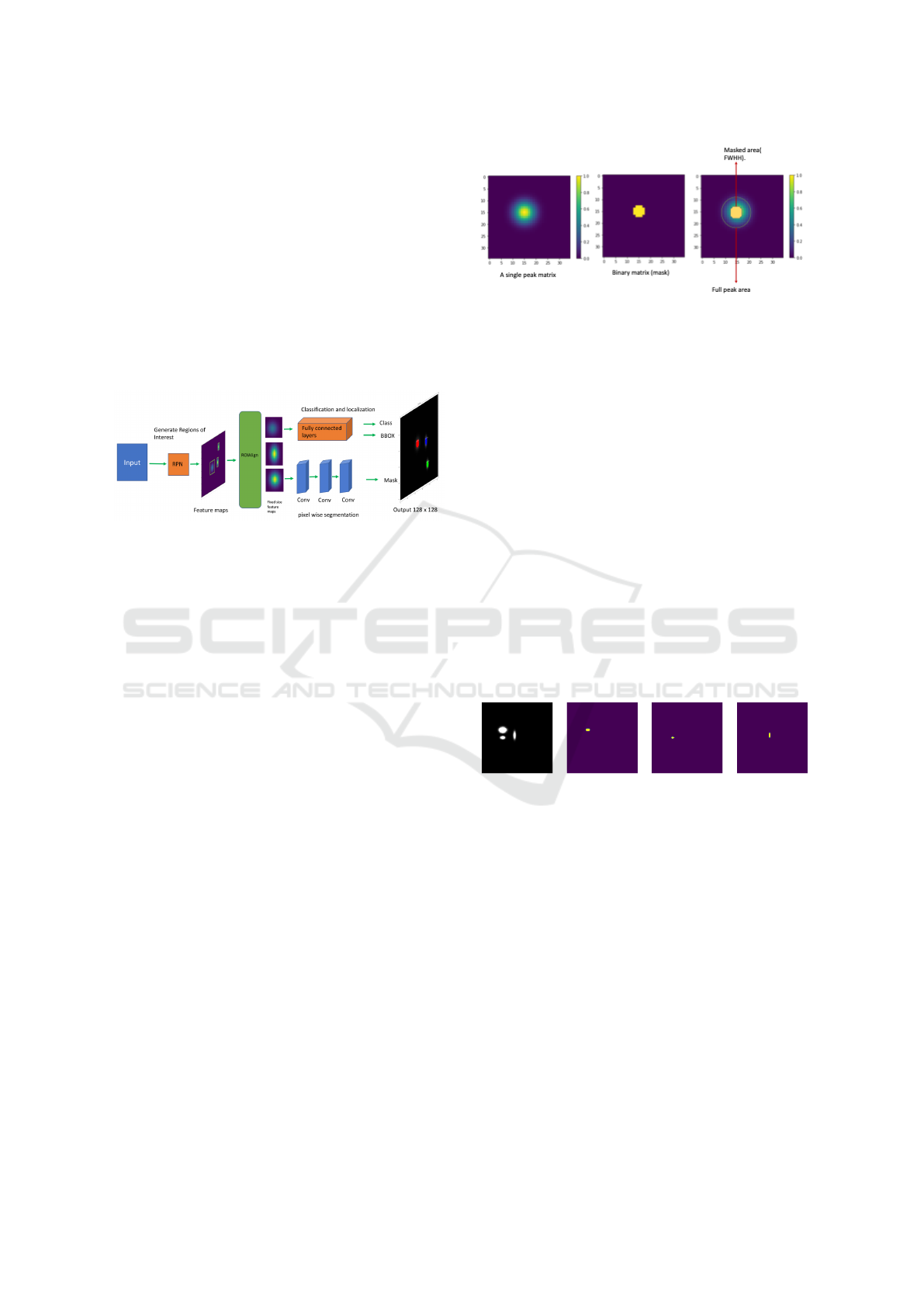
3.2 Mask Calculation
Training data for Mask R-CNN contains two forms of
input, the target objects and corresponding masks.The
masks in our dataset is calculated to cover the area
at full width half height (FWHH) values around each
peak.
Fig. 4 demonstrates the mask area which doesn’t
cover the whole object (peak) as it is the case in most
object detection projects.
Figure 4: Mask covers only FWHH area.
3.3 Dataset
The dataset is synthetically generated using NMRglue
(Helmus and Jaroniec, 2013),a python library pack-
age for NMR analysis. Each generated spectrum con-
tains a number of peaks with the following properties:
1. Spectra are generated as matrices of 64-bit floats.
2. Each matrix has a shape of 128x128 (minimum
size for Mask R-CNN(He et al., 2017).
3. Each matrix contains k peaks randomly located.
where k = [1..4] with uniform distribution.
4. The peaks are either Gaussian at both axis or
Gaussian at one axis and Lorentzian at the other.
5. Maximum amplitude = 1.
6. Masks are calculated to cover the area of full
width half height (FWHH) values around each
peak (local maximum) (see Fig. 5 for an illustra-
tion).
Figure 5: Three peaks and their masks.
7. No noise present during the training.
8. No overlapping masks present.
3.4 Pre-Processing
Mask R-CNN have been primarily applied to the
recognition of natural images, which feature perspec-
tive (distance-size dependence, e.g. objects placed
further appear smaller), fixed aspect ratio and are reg-
ular grids of discrete-value pixels (0–255 in RGB
space). Mask R-CNN applies some standard prepos-
sessing procedures (He et al., 2017)to the input data
such as:
1. Non-square data is resized to square shape by Re-
size and pad with zeros to get a square shape.
2. Inputs must have three channels.
ICAART 2023 - 15th International Conference on Agents and Artificial Intelligence
942
3. Input data is converted to 32-bit floats followed
by subtraction of mean value. Post training, mean
value is added back and data is converted to 8-bit
integers.
4. Batch Normalization Layers are frozen by default.
The model was trained in two implementation scenar-
ios where the first one as standard as possible and the
second one with sensible changes better suited to the
nature of our data.
3.5 Evaluation Criteria
For evaluation of the results of training we use mAP
measure and the rates of False Positive (FP) and False
Negative (FN) detections. mAP is a evaluation metric
used in Mask R-CNN for object localisation and clas-
sification(Everingham et al., 2010). The definitions of
FP and FN should take into account not only predicted
classes but also the locations of predicted bounding
boxes. Hence we define TP, FP, FN as follows. In
Mask-R-CNN the predicted detection {(b
j
, c
j
, p
j
)}
indexed by object j consists of:
• Bounding Box (BB) b
j
,
• predicted class (‘peak’ or ‘no peak’ in our case)
c
j
,
• confidence score p
j
.
A predicted detection (b, c, p) is regarded as a True
Positive (TP) if:
• The predicted category c equals the ground truth
label c
g
.
• The overlap ratio IOU (Intersection Over
Union)(Everingham et al., 2010).
IOU(b, b
g
) =
area (b ∩b
g
)
area (b ∪b
g
)
between the predicted bounding box b and the
ground truth bounding box b
g
is not smaller than a
predefined threshold ε. A predicted detection (b, c, p)
is regarded as a False Positive (FP) if:
• shared a ground truth with another detection (i.e
both predicted detection have IOU with the same
ground truth bounding box in excess of ε) which
has higher confidence score p
j
, or
• has no ground truth bounding box with IOU
greater than ε.
A False negative (FN) is detected if:
• a ground truth peak is found without predicted
bounding box with IOU greater than ε
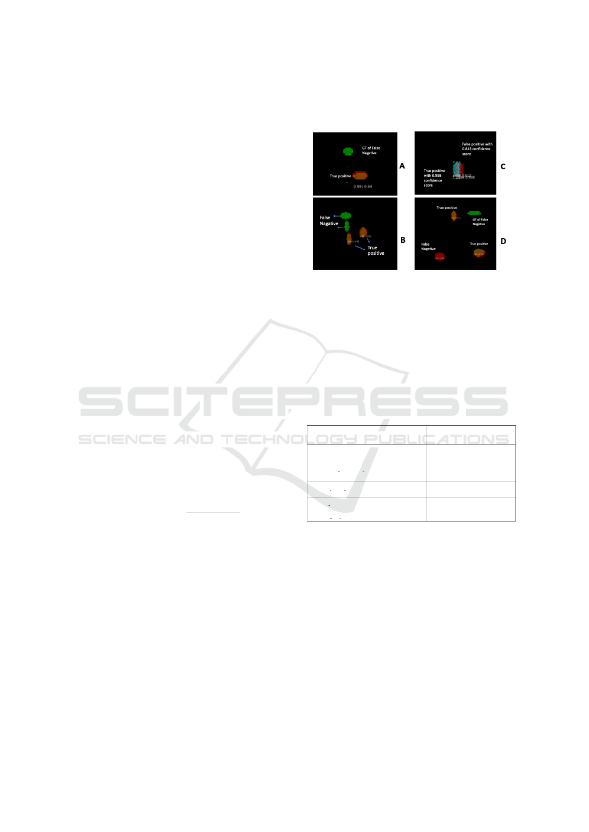
The occurrences False Positives and True Posi-
tives detections are illustrated in Fig. 6.
Figure 6: A, B, C and D display TP, FP and FN in different
scenarios.
4 STANDARD
IMPLEMENTATION
We use the implementation of Mask-R-CNN avail-
able at (He et al., 2017). The model hyper parameters
are listed in Table 1.
Table 1.
Hyper parameters Value Definition
BACKBONE resent50
The backbone networks
DETECTION MIN CONFIDENCE 0.9
Minimum confidence threshold
to accept the final detected ROI
CHANNEL NUMBER COUNT 3
number of channel is 3 for RGB
In our case, we kept it 3 by replicating
the same channel three times
IMAGE MAX DIM 128 x 128
Define input image
resizing (none)
TRAIN BN Freeze
Train or freeze batch
normalization layers
Number OF EPOCHS 20 - 90
define the number of epochs
4.1 Detection Results
Starting with 700 spectra data size, and the Testing
method used here is the traditional 20/80 split. The
model scored a mAP of 0.660 with 2.15 % of FPs
and FNs 19 % of FNs. More detailed analysis was
conducted of the detected peaks by extracting their
details such as height, width and data mean of a whole
spectra, they fall into three categories:
• Correctly Detected Peaks: peaks with maximum
value >= 3.4 are correctly detected and classified.
• Valid peaks with overlapped false peaks: valid
peaks with corresponding Ground Truth GT, those
peaks have also false overlapped peaks.
Detecting 2D NMR Signals Using Mask RCNN
943
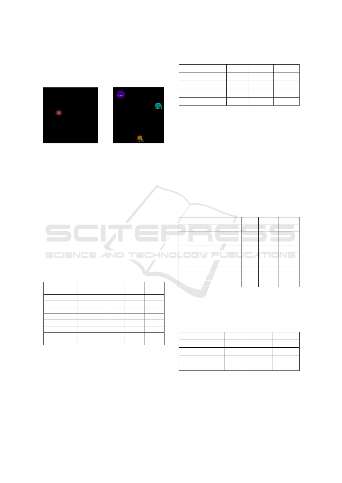
• Not Detected Peaks: missed peaks where they
have GT, but the model failed to detect them.The
majority of the those peaks have maximum value
<= 3.4.
Figure 7: Detected peaks.
To better understand the detection results and im-
prove the accuracy we have applied magnitude scal-
ing for the data. Here we have relied also on the
fact that all essential information in NMR spectra is
magnitude-invariant, that is scaling up or down by a
constant factor does not change the information con-
tent of NMR spectra, but it may well affect the per-
formance of machine learning algorithms on the data.
In practice one can also should take into account the
scaling limitations caused by a particular implemen-
tation (e.g by the range of datatype values available).
In Table 2 we represent the detection results
for various scaling factors applied to testing phase
only.Then the range mean is calculated. The range is
defined here as the difference between the maximum
and minimum values for each spectra then taking the
mean of those values for whole testing dataset.
Table 2.
Scaling factor Range mean mAP FPs % FNs %
No scaling 0.697 0.660 2.150 19.120
5 3.785 0.751 2.370 9.762
10 7.350 0.769 1.280 7.710
15 11.010 0.771 1.080 7.310
50 34.900 0.817 2.720 7.900
100 69.000 0.815 3.000 8.700
150 97.560 0.841 0.540 7.560
200 145.230 0.813 1.560 6.510
255 177.450 0.781 2.460 8.760
As seen from the table the model started preform-
ing better when the data mean between 34.90 and
177.23.Since the scaling was only applied during test-
ing and to form a complete conclusion,Table 3 shows
the outcomes of training the model with scaling dur-
ing: both training and testing, training only and test-
ing only.The scaling factor is determined by selecting
the best preformed model from Table 2 which is 150.
Table 3.
Scaling applied mAP FPs % FNs %
No scaling 0.660 2.150 19.120
Train & Test 0.898 6.480 6.940
Train only 0.579 8.5 13.9
Test only 0.781 2.460 8.760
Scaling during testing only or training and testing
combined show similar results.
4.2 Larger Dataset Size
To eliminate the possibility of inefficient number
of training samples,we generated bigger dataset (5k
spectra).The dataset description and hyper parame-
ters are the same as 700 spectra data size. The model
scored a mAP of 0.616 with 12.15% of FPs and FNs
31% of FNs. Table 4 presents the scaling results dur-
ing the testing stage, and it displays decline in FP
and FN percentage when the data ranges from 2.52
to 7.104 and an increase in mAP score
Table 4.
Description Range mean mAP FPs % FNs %
No scaling 0.5002 0.616 12.19 31.55
5 2.5200 0.630 12.01 9.81
10 4.7690 0.684 10.61 8.90
15 7.1040 0.686 9.10 11.55
50 25.4770 0.557 8.36 21.25
100 48.8730 0.549 8.09 17.78
150 73.1000 0.489 12.32 20.24
200 100.7300 0.464 10.82 18.67
255 122.4400 0.492 11.59 16.60
Similar to the 700 dataset, scaling was also ap-
plied during the three stages. However, scaling during
training and testing combined outperformed the other
scenarios as shown in Table 5.
Table 5.
Scaling applied mAP FPs % FNs %
No scaling 0.616 12.19 31.55
Train & Test 0.784 7.27 2.59
Train only 0.781 3.19 16.66
Test only 0.492 11.59 16.60
Finally,The two best preformed models are se-
lected by scaling to the optimal data range and trained
with the optimal number of epochs see Table 6.
• Scaling of the range mean between 83.23 and
122.7.
ICAART 2023 - 15th International Conference on Agents and Artificial Intelligence
944
• Scaling in both the training and testing stages.
Table 6.
Data size mAP FPs % FNs %
700 0.788 0.400 1.200
5k 0.971 1.160 2.320
5 ADJUSTED IMPLEMENTATION
As mentioned in the previous section, most unde-
tected peaks that have maximum value <= 3.4. Those
peaks are relatively small and that might be a reason
for low performance of Mask R-CNN standard imple-
mentation. In order to improve performance we have
made several changes to the framework.
5.1 Modified Normalization
The default Mask R-CNN pre-processing in explained
in Section III-D, converts floats into integers directly
causing the values to be floored to 0.In order to pre-
serve the data the pre-processing was modified. Fig.8,
shows the effects of standard normalization (upper
part) and modified normalization (bottom part). The
bottom part of the figure shows the modified method
where the subtraction of zeros (instead of mean value)
and the conversion to original datatype (float64) in-
stead to unint8 has been applied.
Standrad
Modified
Input loading
• Converting to float
• Substrating mean values
• Adding mean values
• Converting to unint8
Input loading
• Converting to float
• Substrating (zeros)
as mean values.
• Adding mean values
• Converting to oringial
datatype ( float64)
• Read original as Float64 matrix
• Convert to flaot32
• Substract MEAN PIXEL Values.
Results:
• Convert to int8
Results:
• Read original as Float64 matrix
• Convert to flaot32
• Substract MEAN PIXEL Values.
Results:
• Convert to int8
Results:
• Read original as Float64 matrix
• Convert to flaot32
• Substract MEAN PIXEL Values.
Results:
• Convert to int8
Results:
• Read original as Float64 matrix
• Convert to flaot32
• Substract MEAN PIXEL Values.
Results:
• Convert to int8
Results:
• Read original as Float64 matrix
• Convert to flaot32
• Substract MEAN PIXEL Values.
Results:
• Convert to int8
Results:
• Read original as Float64 matrix
• Convert to flaot32
• Substract MEAN PIXEL Values.
Results:
• Convert to int8
Results:
Figure 8.
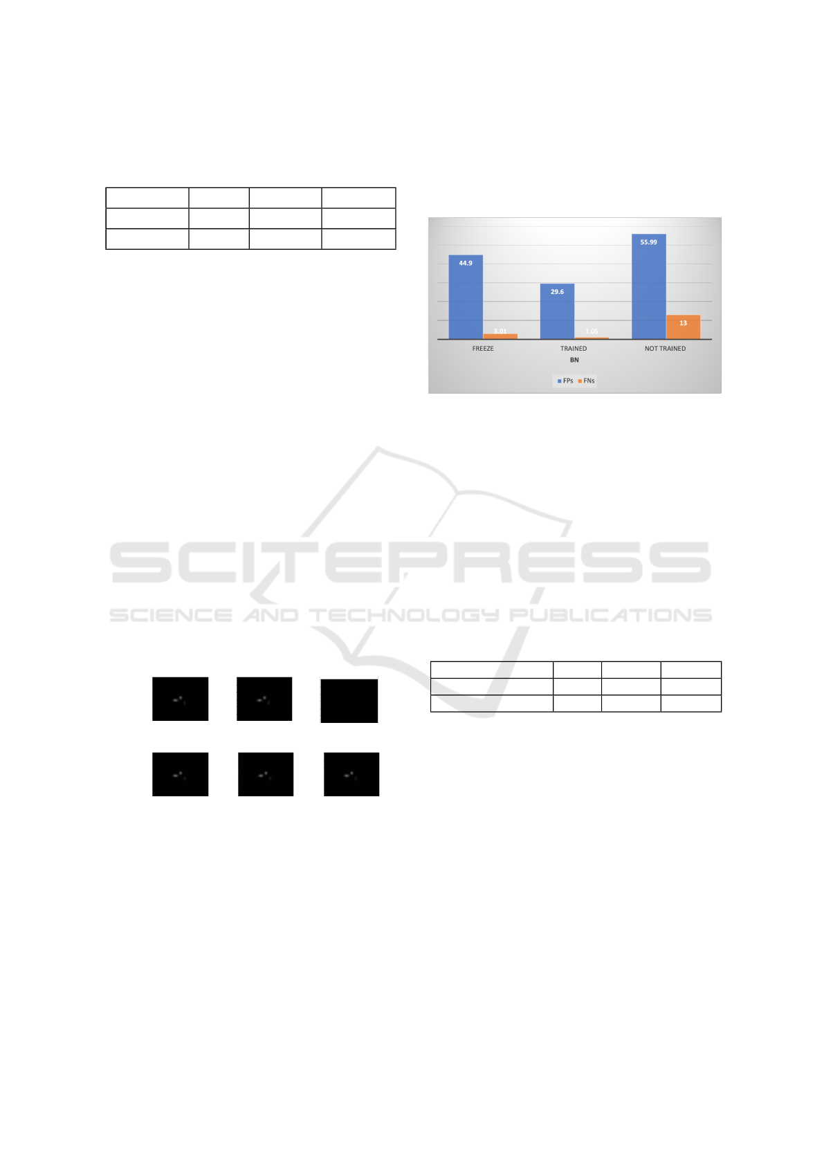
5.2 Batch Normalization Layers
Mask R-CNN’s default Batch normalization (BN)
layer setting are to freeze during training and used
during predicting phase where the mean values
provided in configuration file subtracted from the
data.Here, we experimented to determine in our set-
tings whether to freeze, train or use BN layers in train-
ing mode during prediction.The detection results have
improved significantly by training the BN layers, as
shown in Fig. 9.
Figure 9: BN Layers tests.
5.3 Input Normalization
Mean values are used in Mask-RCNN for input nor-
malization. Here we tested whether to use the cal-
culated mean values or standard deviation for input
normalization is better for our datatype. The model is
trained with:
• 90 epochs.
• The BN layers are trained.
• The STD and Mean values are calculated across
the dataset (5k).
Table 7.
Input normalization mAP FPs % FNs %
calculated mean 0.91 35.50 0.46
calculated Std 0.93 10.17 1.79
The results of experiments are shown in the Table
7.They indicate the advantage of using STD for in-
put normalization as as in this case the model demon-
strates good performance with only 10.17 % FPs and
only 1.7 % FNs. Fig. 10 displays the final Mask R-
CNN model for peaks detection and segmentation of
2D NMR spectra which gives 0.93 mAP with 10.17%
FPs and only 1.79% FNs.
6 DISCUSSION
In this paper, we are presenting an implementation of
Mask R-CNN for 2D NMR peak picking trained with
synthetic data.We have evaluated the default setting
used in image segmentation for NMR data. Our find-
ings showed us that although NMR data can be treated
Detecting 2D NMR Signals Using Mask RCNN
945

Figure 10: NMR Mask-RCNN Model.
as an image the defaults used in Mask R-CNN does
not perform sufficiently. We have opted for avoid-
ing data type conversions in order to preserve the in-
formation in the NMR data which were initially lost.
Following hyper-parameter tuning, we observed poor
detection on low intensity peaks. In order to increase
our detection, we implemented uniform scaling on the
data matrix during training. In this further improved
pipeline we have achieved greater performance with
0.90 mAP, 10.17% FP and 1.7% FNs with a scaling
factor of 150. The necessity of scaling is most likely
due to the nature of the NMR data. Regular pictures
have very clear borders between object; in the case
of NMR, the objects (peaks) in the picture (spectra)
has gradually disappearing borders. When the object
of interest is intrinsically smaller (low intensity peak),
it is particularly challenging to differentiate between
the baseline, borders and the maxima. Thus, applying
some prior to training can make these feature more
detectable by Mask R-CNN. Our conclusion is that
this framework is promising and needs further inves-
tigations. Further directions include in particular con-
sidering more realistic spectra with multiple possibly
overlapping peaks and testing on both synthetic and
real experimental data.
REFERENCES
Cheng, Y., Gao, X., and Liang, F. (2014). Bayesian
peak picking for nmr spectra. Genomics, pro-
teomics & bioinformatics, 12(1):39–47 doi:
10.1016/j.gpb.2013.07.003. Epub 2013 Oct 31.
PMID: 24184964; PMCID: PMC4411369.
Chiao, J.-Y., Chen, K.-Y., Liao, K. Y.-K., Hsieh, P.-H.,
Zhang, G., and Huang, T.-C. (2019). Detection
and classification the breast tumors using mask r-
cnn on sonograms. Medicine, 98(19):e15200. doi:
10.1097/MD.0000000000015200. PMID: 31083152;
PMCID: PMC6531264.
Corne, S. A., Johnson, A. P., and Fisher, J. (1992). An ar-
tificial neural network for classifying cross peaks in
two-dimensional nmr spectra. Journal of Magnetic
Resonance (1969), 100(2):256–266.
Davis, C. C., Champ, J., Park, D. S., Breckheimer, I., Lyra,
G. M., Xie, J., Joly, A., Tarapore, D., Ellison, A. M.,
and Bonnet, P. (2020). A new method for counting
reproductive structures in digitized herbarium spec-
imens using mask r-cnn. Frontiers in Plant Sci-
ence, 11:1129 doi: 10.3389/fpls.2020.01129. PMID:
32849691; PMCID: PMC7411132.
Elyashberg, M. (2015). Trac trends anal. Struc-
ture–Spectrum Correlations and Computer-Assisted
Structure Elucidation Joao Aires de Sousa.
Everingham, M., Van Gool, L., Williams, C. K., Winn, J.,
and Zisserman, A. (2010). The pascal visual object
classes (voc) challenge. International journal of com-
puter vision, 88:303–338.
Goddard, T. and Kneller, D. (2007). Sparky 3 . san fran-
cisco: University of california.
He, K., Gkioxari, G., Dollar, P., and Girshick, R. (2017).
”mask r-cnn”. Mask r-cnn. In, 2017 IEEE Interna-
tional Conference on Computer Vision (ICCV), pages
2980–2988 doi: 10.1109/ICCV.2017.322.
Helmus, J. J. and Jaroniec, C. P. (2013). Nmr-
glue: an open source python package for the anal-
ysis of multidimensional nmr data. Journal of
biomolecular NMR, 55:355–367 http://dx.doi.org/10.
1007/s10858--013--9718--x.
Hesse, R., Streubel, P., and Szargan, R. (2007). Prod-
uct or sum: Comparative tests of voigt, and prod-
uct or sum of gaussian and lorentzian functions in
the fitting of synthetic voigt-based x-ray photoelec-
tron spectra. Surface and Interface Analysis: An In-
ternational Journal devoted to the development and
application of techniques for the analysis of surfaces,
interfaces and thin films, 39(5):381–391.
Johnson, B. A. and Blevins, R. A. (1994). Nmr view: A
computer program for the visualization and analysis
of nmr data. Journal of biomolecular NMR, 4(5):603–
614.
K., W. (1986). Nmr of proteins and nucleic acids’,
new york: John wiley and sons, [online].
https://www.europhysicsnews.org/articles/epn/
pdf/1986/01/epn19861701p11.
Klukowski.P and al (2015). Computer vision-based auto-
mated peak picking applied to protein nmr spectra.
Bioinformatics, pages 2981–2988.
Li, D.-W., Hansen, A. L., Yuan, C., Bruschweiler-Li, L.,
and Br
¨
uschweiler, R. (2021). Deep picker is a deep
neural network for accurate deconvolution of complex
two-dimensional nmr spectra. Nature communica-
tions, 12(1):5229. doi: 10.1038/s41467–021–25496–
5. PMID: 34471142; PMCID: PMC8410766.
Liu, Z., Abbas, A., Jing, B.-Y., and Gao, X. (2012).
Wavpeak: picking nmr peaks through wavelet-based
smoothing and volume-based filtering. Bioinformat-
ics, 28(7):914–920.
Pellecchia, M., Bertini, I., Cowburn, D., Dalvit, C., Giralt,
E., Jahnke, W., James, T. L., Homans, S. W., Kessler,
H., Luchinat, C., et al. (2008). Perspectives on nmr in
drug discovery: a technique comes of age. Nat Rev
ICAART 2023 - 15th International Conference on Agents and Artificial Intelligence
946

Drug Discov, 7(9):738–745 doi: 10.1038/nrd2606.
PMID: 19172689; PMCID: PMC2891904.
SP, S., R, F., W, B., TJ, R., LG, M., and GW, V. (2016). Ccp-
nmr analysisassign: a flexible platform for integrated
nmr analysis. Journal of Biomolecular NMR.
Tikole, S., Jaravine, V., Rogov, V., D
¨
otsch, V., and G
¨
untert,
P. (2014). Peak picking nmr spectral data using
non-negative matrix factorization. BMC bioinformat-
ics, 15:46 doi: 10.1186/1471–2105–15–46. PMID:
24511909; PMCID: PMC3931316.
Zhao, K., Kang, J., Jung, J., and Sohn, G. (2018). Build-
ing extraction from satellite images using mask r-cnn
with building boundary regularization. In IEEE/CVF
Conference on Computer Vision and Pattern Recog-
nition Workshops (CVPRW), pages 242–2424 doi:
10.1109/CVPRW.2018.00045.
Detecting 2D NMR Signals Using Mask RCNN
947
