Noise Robustness of Data-Driven Star Classiﬁcation

Floyd Hepburn-Dickins

and Michael Edwards

Department of Computer Science, Swansea University, U.K.

Keywords:

Neural Networks, Star-Pattern Recognition, Data Generation.

Abstract:

Celestial navigation has fallen into the background in light of newer technologies such as global positioning

systems, but research into its core component, star pattern recognition, has remained an active area of study.

We examine these methods and the viability of a data-driven approach to detecting and recognising stars within

images taken from the Earth’s surface. We show that synthetic datasets, necessary due to a lack of labelled real

image datasets, are able to appropriately simulate the night sky from a terrestrial perspective and that such an

implementation can successfully perform star patter recognition in this domain. In this work we apply three

kinds of noise in a parametric fashion; positional noise, false star noise, and dropped star noise. Results show

that a pattern mining approach can accurately identify stars from night sky images and our results show the

impact of the above noise types on classiﬁer performance.

1 INTRODUCTION

Star pattern recognition dates back to the ancient era,

used by a multitude of empires as part of naviga-

tion for exploration and trade. Polynesia, one of

the worlds largest nations at its time, was formed in

great part due to celestial navigation. This is achieved

through the use of guiding stars and constellations,

man-made groupings of stars easily picked out due

to them containing those brightest and most obvious

stars in the night sky. The advent of modern com-

puting has supplanted these methods through a host

of alternative navigation systems, most predominately

global positioning systems. There is still a call for

celestial navigation, most often with regard to space

borne vessels and attitude determination (Rijlaarsdam

et al., 2020; van Bezooijen, 1989). In recent years,

when considering a desire for greater redundancy in

navigational systems and the potential threats posed

towards global position systems from the vulnerabil-

ity of the satellites themselves to the possibility of

interference from third parties, celestial navigation

presents itself as a viable alternative.

At its core exist two primary problems, star de-

tection, that is to pinpoint prospective stars within an

image, and star recognition, the correct identiﬁcation

of a given star. Whilst the former is a widely solved

issue (Stetson, 1987), the latter remains a point of ac-

tive research (Rijlaarsdam et al., 2020). The computer

age has brought with it a host of improvements on this

https://orcid.org/0000-0001-5943-0652

https://orcid.org/0000-0003-3367-969X

ancient art, moving from identifying deﬁned constel-

lations and the stars within, to deriving more general

solutions applicable across the night sky.

Whilst the focus of modern research is more com-

monly applied towards spacecraft and attitude de-

termination, the techniques and methods used can

broadly still be applied to navigation from the Earth’s

surface as well. The ﬁrst and foremost challenge is

essentially the same; any navigation requires the ac-

curate and timely pinpointing and recognition of the

stars at hand. In the past this would be achieved

slowly by consulting a nautical almanac and sextant.

Modern pattern recognition techniques can vastly im-

prove both the acquisition and identiﬁcation and have

been shown to do so when applied to attitude determi-

nation, we further examine their efﬁcacy on systems

grounded to the earths surface alongside the chal-

lenges that entails.

2 RELATED WORK

Despite fading into the background of navigation, star

identiﬁcation and recognition has nonetheless seen

a steady evolution of research over the decades. In

(Liebe, 1993) they proposed a triangle method, form-

ing patterns based on the angular distances between a

triplet of stars, the spherical angles between them and

their magnitudes. By generating a database of these

geometric properties and the patterns they form they

are able to match prospective identiﬁcations against

them and thus identify a given star. The method is

176

Hepburn-Dickins, F. and Edwards, M.

Noise Robustness of Data-Driven Star Classiﬁcation.

DOI: 10.5220/0011804000003411

In Proceedings of the 12th International Conference on Pattern Recognition Applications and Methods (ICPRAM 2023), pages 176-184

ISBN: 978-989-758-626-2; ISSN: 2184-4313

 2023 by SCITEPRESS – Science and Technology Publications, Lda. Under CC license (CC BY-NC-ND 4.0)

both rapid and accurate, but suffered limitations with

the introduction of false stars, a problem ever more

apparent due to the crowding of the celestial sphere

with satellites and other man-made objects that may

present themselves in an image. This was improved

upon in (Nabi et al., 2019) via their design of the star-

triplet database construction and feature extraction

methods resulting in a greater tolerance to missing

stars and improved ability in handling reduced num-

bers of stars present within the ﬁeld of view (FOV).

There are a number of papers based around these

handcrafted properties between a guiding reference

star (GRS) and its guiding neighbour stars (GNS).

The work of (Mortari et al., 2004) utilised a pyramid

schema of four stars able to resist larger numbers of

false stars. The speed can then be increased via the

use of hash mapping with the pyramid method when

searching the space of available patterns (Wang et al.,

2018) .

The grid based algorithm (Padgett and Kreutz-

Delgado, 1997) utilises a primary star and its neigh-

bours within a speciﬁed radius to form a pattern vec-

tor, providing greater tolerance towards positional

noise. The modiﬁed grid algorithm (Na et al., 2009)

further increased position and magnitude tolerance.

Additional work here includes the use of radial and

cyclical feature patterns (Zhang et al., 2008) allow-

ing for rotation-invariant matching. With (Jiang et al.,

2015) improving upon the radial patterns and their po-

sitional tolerance via utilising a redundant-coded so-

lution.

Machine learning techniques in the work of (Xu

et al., 2019) have utilised these pattern generation

techniques through the lens of neural networks. This

allows for the use of machine learned patterns in lieu

of the handcrafted ones in prior literature, eliminat-

ing the need to search through any datasets for pattern

matching whilst (Yang et al., 2022) utilises a 1D con-

volutional neural network to achieve increases in both

speed and robustness towards various noise types.

Throughout this paper we examine the auto-

encoder and classiﬁer outlined in (Xu et al., 2019) and

its performance when operating on simulated images

from the earths surface whilst parametrically explor-

ing the models tolerance to noise.

3 PROPOSED METHODOLOGY

3.1 Detection from Image

In order to recognise the stars they must ﬁrst be de-

tected within an image. This involves accurately pin-

pointing the centre of a source, minimising the de-

tection of false sources and overcoming the varying

noise that may be present. To do this, we use an

implementation of the DAOFIND algorithm (Stetson,

1987) that searches an image for local density max-

ima with a peak amplitude exceeding a chosen thresh-

old and whose size and shape are similar to a deﬁned

2D Gaussian kernel. Through this we can apply vari-

ous thresholds and parameters relating to the the size

and intensity of prospective sources in order to ﬁlter

relative to our domain and conditions. By subtracting

the median of our image prior to entering it into the

algorithm, we can reduce the impact of background

noise and light pollution, an issue that is much more

prevalent in our domain of ground-borne wide angle

sensors.

This allows for the accurate pinpointing of

prospective sources centroids, which can then be used

as the basis for the data our model will see. Whilst

some stars will inevitably be lost, some centroids may

be off by a small amount, and false stars will still ﬁlter

through and become included in our detected sources,

these are precisely the types of noise we hope to build

a tolerance to within our implementation.

3.2 Constellation Representation

Figure 1: Pipeline.

Moving from detected sources to a classiﬁcation ﬁrst

requires a learned representation of each star within

our catalogue. To do this we need to extract informa-

tion about the local features for each star. The exact

deﬁnition of what is local for a star depends on our

chosen parameters. We opt to utilise those stars clos-

est to a prospective GRS as they are more likely to be

captured together in an image.

When considering a given star and its neighbours,

the primary points of information we can utilise are

the brightness of the stars, and more critically, the lo-

cal topology of points, speciﬁcally the angular dis-

tances between them. By utilising the angular dis-

tances between the stars in a radial manner we are

able to make our learned representation invariant to

rotation and translation within the image. The angu-

lar distance will remain constant, across images and

time, forgiving the minor shifts in the stars them-

selves, thankfully this takes place over such a span

of time as to be negligible.

The night sky is rarely perfectly clear, showing us

just the stars as we want them. There is a great deal of

noise, from occlusion and light pollution to all manner

Noise Robustness of Data-Driven Star Classiﬁcation

177

of satellites and astronomical phenomenon that may

be present across our view. Beyond that, the imag-

ing system itself can introduce errors or noise. To in-

crease the robustness of our classiﬁer it needs to over-

come this noise, and as such we train our classiﬁer

on a variety of simulated noisy conditions categorised

as positional noise, false star noise and dropped star

noise.

Positional noise occurs when the reported centroid

of the star is inaccurate, typically to the degree of a

pixel or so, as a result of centroid detection in un-

clear images. False star noise occurs when we detect

and attempt to both classify, and use in the classiﬁ-

cation of other sources, false sources. Such sources

aren’t stars within our image and are typically borne

about through stellar artefacts or phenomenon such

as passing satellites, aircraft or meteorites. Dropped

star noise is where sources that should be present in

the image and used for classiﬁcation are omitted, typ-

ically due to occlusion of part of the image from some

terrestrial artefact or weather conditions.

By introducing this noise into our training images,

we can imbue a tolerance towards it in our eventual

classiﬁer. Such images can reduced into lists, D

and D

, detailing the distances between a GRS and

it’s nearby GNSs and the pair-wise distances between

GNSs respectively. The discretized outcome of these

lists, concatenated together to preserve identity be-

tween them, forms the input for our model, that which

is used to discern a star pattern or representation.

The parameters for the radius, from which we con-

sider GNSs, and discretization can be varied but in

keeping with the results from (Xu et al., 2019) and

experimental testing we use an input dimension of

400, derived form a radius p and discretization factor

e where p/e = 200. The model is trained by creating a

clean tensor and several noisy counterparts.

Clean tensors are formed utilising the Yale Bright

star catalogue (BSC), or a magnitude threshold-ed

version thereof, by choosing a star and retrieving all

neighbouring stars within p. Each star is represented

as a declination and right ascension and from these

values we can calculate D

and D

, and thus the in-

put tensor.

3.3 Constellation Recognition

Recognition refers to the ﬁnal step, the determination

of precisely which star our input tensor refers to. The

star pattern generator maps from a potentially noisy

input to an approximation of the clean tensor for that

star. We then train a classiﬁer to take these tensors

and learn the association between them and its classi-

ﬁcation, in our case its HR designation. For a given

vector we obtain a probability it belongs to each of

the stars in out catalogue, we then take the highest

probability result as our classiﬁcation.

4 EXPERIMENTAL SETUP

4.1 Datasets

4.1.1 Training Data

In order to train the autoencoder we require a clean

constellation representation and multiple noisy vari-

ants. Clean representations are obtained using the

BSC, a catalogue of stars visible to the naked eye,

ranging up to a visible magnitude of 6.5. From this

we extract the HR number, DECJ200, RAJ2000, and

visible magnitude to form a simpliﬁed revised cata-

logue.

After selecting a candidate star from the BSC cat-

alog we identify those stars that fall within our cho-

sen radius p and generate the clean tensor input via

discretizing D

and D

. In order to create noisy

counterparts we utilise a data augmenter during the

training of the star pattern auto-encoder. This aug-

menter randomly applies a noise type and intensity to

the prospective star and its connected stars within p

before re-calculating and re-sorting the angular dis-

tances in order to generate D

and D

for this new

noisy variant. The structure of the data augmenter is

shown in ﬁgure 2.

Dropped star noise is created by randomly choos-

ing between 1 and a pre-determined maximum num-

ber from the neighbouring stars and removing them

from the set.

False star noise is created by applying a random

angular offset between 0

◦

and 360

◦

from the central

star, as well as a random separation offset between 0

◦

and the radius p to create a new star. The new stars

RA and DEC is then calculated as an offset from the

focal star.

Position noise chooses a random angular offset

from 0

◦

-360

◦

and a separation offset from 0

◦

−x ∗

radius where x is our chosen modiﬁer for the max-

imum potential offset. Each star is then shifted ac-

cording to these values.

Once noise has been applied, angular distances

between stars are re-calculated and the list of near-

est neighbours re-sorted before discretiziation. Ulti-

mately this process allows for the stochastic genera-

tion of noisy counterparts for each stars clean tensor.

ICPRAM 2023 - 12th International Conference on Pattern Recognition Applications and Methods

178

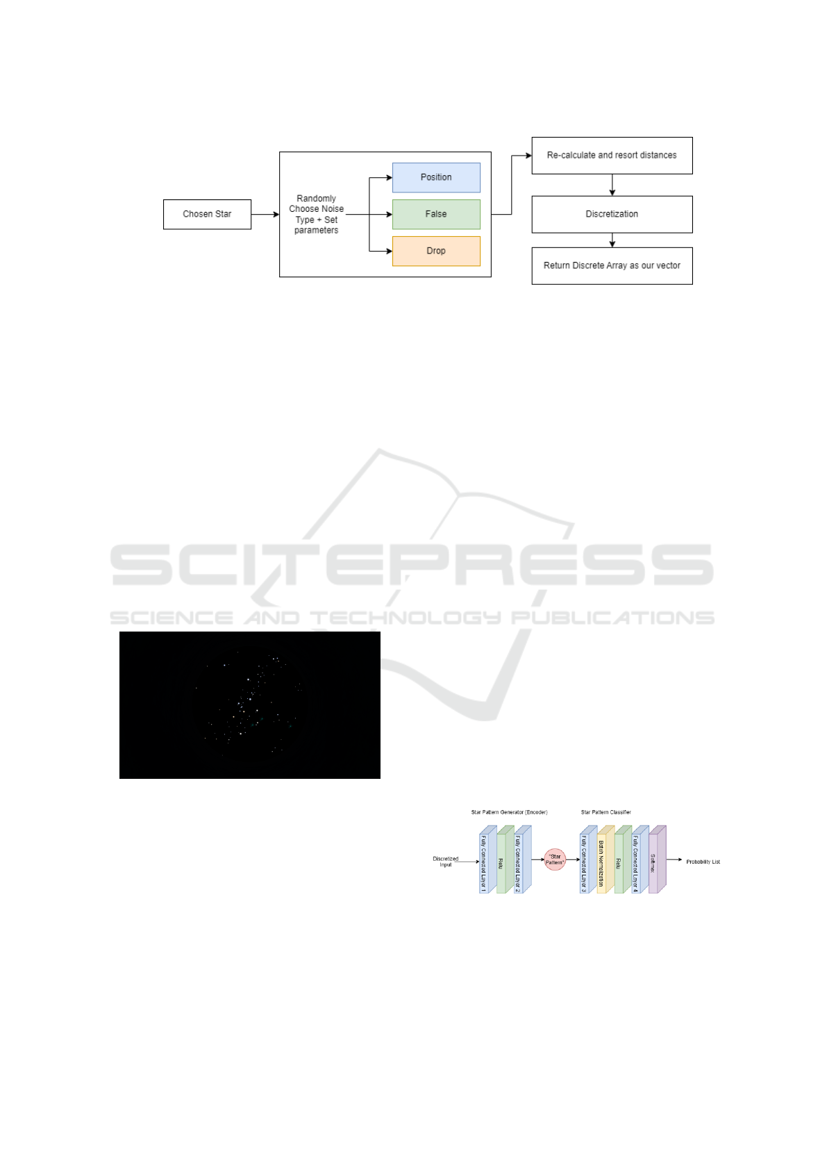
Figure 2: Data augmenter.

4.1.2 Testing Data

In order to validate our approach we utilise the open

source software Stellarium to obtain synthetic images

of the night sky. Through this we can emulate a par-

ticular viewpoint and simulate the stars up to a desired

visible magnitude. We can furthermore include or re-

move any celestial artifacts, ambient light pollution

and satellites within the environment to garner clearer

or more realistic images.

For each synthetic image we extract the pixel co-

ordinates of each star alongside the catalogue infor-

mation from the BSC. This results in each image hav-

ing a corresponding CSV ﬁle detailing the metadata

for the viewpoint, j-date, camera origin and details for

each star.

For our testing we generated 11900 such images,

randomly sampling longitudinal and latitudinal points

across the Earth’s surface.

Figure 3: A synthetic image generated within Stellarium.

4.2 Implementation

Source detection is achieved utilising DAOStarFind

from the astropy library. Prior to performing the op-

eration on the image, we subtract the median value

from it in order to reduce background noise. This pro-

vides us with a list of sources typically exceeding the

actual number of stars present in the image, due to the

detection of satellites and other false stars.

In order to generate our model input we need to

be able to convert from pixel to angular distances. In

lieu of calibrating a camera we train a support vector

machine (SVM) to map from the pixel co-ordinates

of a star to its angular distance to the centre of the

image. We are able to train the SVM from the CSV

ﬁles generated alongside our synthetic images.

By imagining the centre of the image as being

right ascension 0 and declination 0 we can determine

a supposed RA/DEC of a particular star by calculating

it is an offset from this central point, calculating the

distance using our SVM. Whilst the RA/DEC is unre-

lated to its true RA/DEC, we can utilise these manu-

factured values alongside those of another star in the

same frame to calculate the angular distance between

them, which would be the same for their true right as-

cension and declination, thus allowing us to generate

our D

and D

lists.

The ﬁnal model used to classify sources is built

from a star pattern generator and star pattern classi-

ﬁer the structure of which is shown in ﬁgure 4. The

generator is the pre-trained auto-encoder created by

training on simulated images of a GRS and its nearby

GNSs. Each GRS has a clean pattern, borne from the

discretization of its angular distance to its GNSs and

the intra-GNS distances. Each clean pattern is aug-

mented using the data augmenter detailed above to

create noisy counterparts of varying intensity for each

of the noise types. In training an auto-encoder to de-

noise these noisy versions we are left with an encoder

capable of creating latent star-patterns for use in our

classiﬁer.

Figure 4: Combined structure of the star pattern generator

and star pattern classiﬁer.

Hyper-parameters were chosen from a mix of

those derived in (Xu et al., 2019), batch testing, and

practical considerations. When considered in the con-

Noise Robustness of Data-Driven Star Classiﬁcation

179

text of navigation on the earths surface, achieved

without expensive imaging systems, we limit magni-

tude down to 3MV on a ﬁsh-eye lens. This allows for

the use of inexpensive cameras, using lower exposure

times whilst trying to capture as much information

as possible. The lower magnitude threshold is borne

from this need for minimal exposure times, to reduce

noise imparted through motion . We still adhere to

the input size arrived at within (Xu et al., 2019) of

200 derived from 2[p/e] as well as utilising 10 GNSs

per GRS, but due to fewer stars being present within

each image we need to expand the radius under which

stars are collected to achieve this. Testing found that

increasing this to 60

◦

allowed for the capture of the

10 GNSs necessitating an increase of the e factor to

0.3. The auto-encoder is trained ﬁrst with a batch size

of 32 before ﬁne tuning with a batch size of 512.

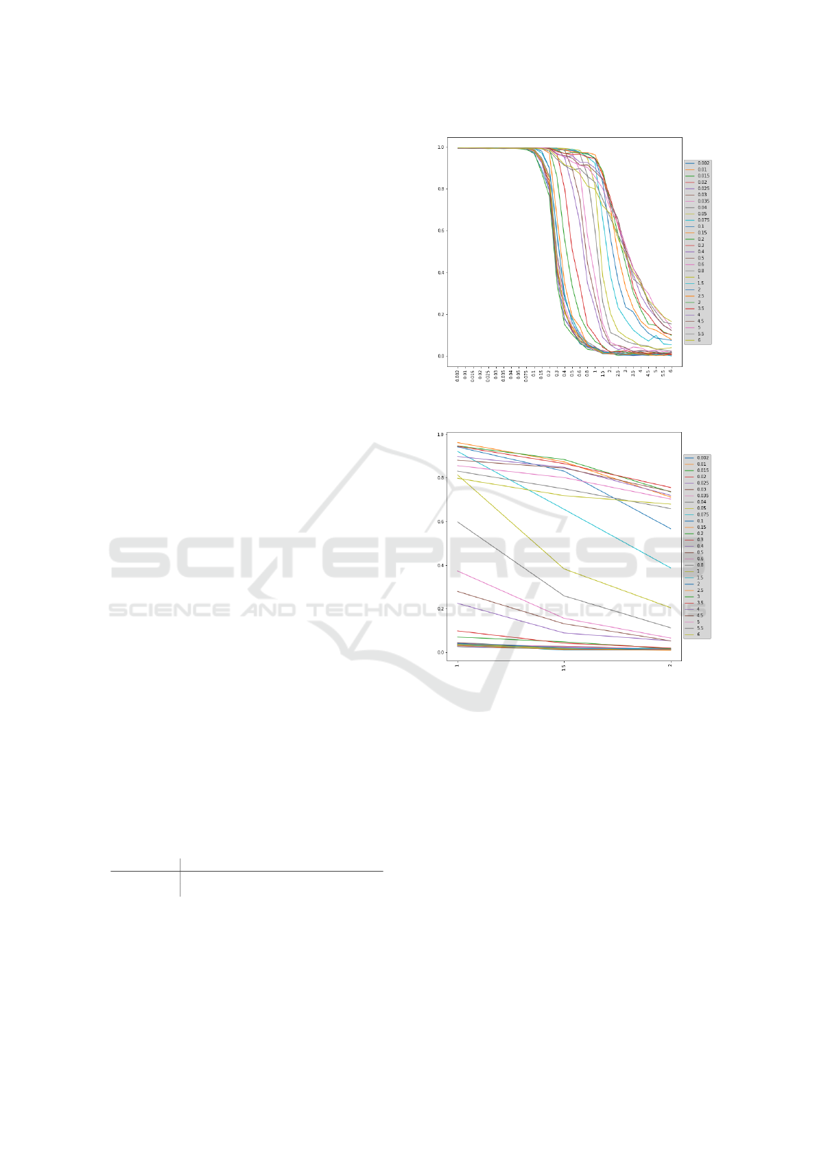
In order to maximise position noise tolerance with

these new imaging parameters we exhaustively tested

training the full model with differing levels of posi-

tion noise applied. From these we can choose the

model that is best able to handle the most position

noise. Training was done via randomly applying po-

sition noise up to a maximum value. This maximum

value was tested up to 6

◦

at which point the accuracy

suffered greatly. In evaluating position tolerance, the

generator was adjusted to generate results only at the

provided value opposed to a range up to that value,

and to only apply position noise rather than the other

types. We then evaluated each model at each position

value allowing us to see the trade-off between toler-

ance to position noise and accuracy. The ﬁrst results

are visible in ﬁgure 5 and ﬁgure 6. The most appro-

priate model from these would be one trained on po-

sition noise up to 2.5

◦

and effective up to 1

◦

with an

accuracy of ∼ 96.2%. However by further examining

potential solutions within the optimal zone we aim to

improve on this preliminary model.

The early results show the best models exist where

they are trained to 2.5 to 3.5 but evaluated up to 1 to

1.5. Subsequently we search with greater granularity

within this space, erring to either side, for the opti-

mal model. This subsequent search parameters are

detailed in Table 1.

Table 1: Model Training Parameters.

Epochs Batch Size Early stopping

Autoencoder 4000 / 2000 32 / 512 No

Classiﬁer 2000 512 Yes

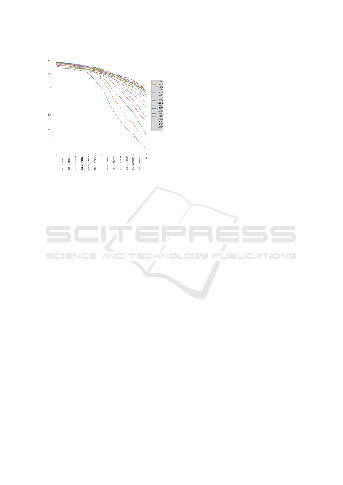
Figure 7 shows the results of the more pinpointed

training under this regime.

Table 2 showcases the results from the further test-

ing to identify the optimal model, trading off toler-

ance towards pixel noise against accuracy, focused on

Noise Testing Value

Model Accuracy

Train

Value

Figure 5: Position noise and its impact on accuracy.

Noise Testing Value

Model Accuracy

Train

Value

Figure 6: Position noise and its impact on accuracy close

up.

due to it being the primary source of noise present

within our simulated images, particularly when con-

sidering the innate error generated when converting

from pixel to angular distances from the SVM. These

results were generated by evaluating the model at ex-

plicitly the stated test value for pixel noise, opposed

to a random distribution up to that value, as they were

trained.

The table shows the best model able to handle the

given test value of pixel noise. The desire is to choose

a model tolerant to as much position noise as possi-

ble, whilst still maintaining a high degree of accu-

racy. To this end, the model trained at 3.342

◦

but vi-

able up to 1.393

◦

is selected to move forward in our

testing. When evaluated across all noise types this

model scores an accuracy of 98.53% on 320000 sam-

ICPRAM 2023 - 12th International Conference on Pattern Recognition Applications and Methods

180

Noise Testing Value

Model Accuracy

Train

Value

Figure 7: Position noise and its impact on accuracy, further

testing.

Table 2: Showcasing the optimal model training value to

maximise accuracy on a given test value when considering

positional noise.

Optimal Training Max Test Value Accuracy

2.157 0.75 0.987

2.157 0.857 0.983

2.553 0.964 0.979

2.947 1.071 0.974

2.947 1.179 0.965

2.816 1.286 0.954

3.342 1.393 0.951

3.737 1.5 0.937

2.947 1.607 0.921

3.737 1.714 0.9

3.342 1.821 0.887

3.737 1.929 0.875

3.342 2.036 0.853

3.737 2.143 0.829

3.737 2.25 0.811

ples generated from the augmenter.

In summation, our ﬁnal model chosen to be tested

on real images has been trained up to noise tolerance

of 3.342

◦

, though practically it is considered accurate

up to a value of 1.393

◦

. The auto-encoder has been

trained across 6000 epochs, 4000 with a batch size of

32 and 2000 with a batch size of 512 for ﬁner adjust-

ments. The classiﬁer is trained for 2000 epochs at a

batch size of 512 with early stopping. Early testing

showed this to be the best batch size for the classiﬁer

and is in-keeping with the ﬁndings of (Xu et al., 2019)

although the datasets are quite different at this point

due to the differing thresholds on magnitude.

5 RESULTS

Before testing the model we can examine the results

of the source detection algorithm. Across 11900 im-

ages simulated in Stellarium with a magnitude thresh-

old of three, 1104659 sources were detected vs the

true value of 1036254 stars being present within

those images. The disparity stems from two primary

sources, the ﬁrst, and most common, is the presence

of stellar phenomenon across many of the images,

most common was various meteor showers that were

detected in images located across the breadth of the

Earths surface, these were subsequently picked up as

one or more sources in each of the images in which

they exist and account for the vast majority of the

discrepancy between actual stars and sources. Ad-

ditional detections stem from certain stars that were

detected as multiple sources, though rarely, as well

as a minor discrepancy between those stars simulated

within Stellarium vs those that were calculated as be-

ing present in the image based off the Yale bright

star catalogue. Namely where Stellarium calculated

a stars apparent magnitude to be different to the cat-

alogue, and where this value pushed a star below our

magnitude threshold, it resulted in stars being shown

that shouldn’t be.

The SVM was trained on the angular distance

from each star in an image to the center of that im-

age. Within the 11900 synthetic images we obtain

1036254 distances. With a train test split of 0.2 it

scored an accuracy of ∼ 0.9988 with an average error

of 0.05

◦

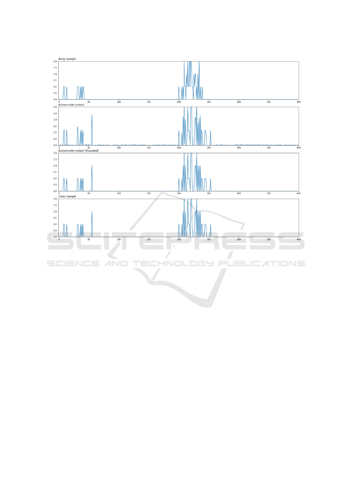
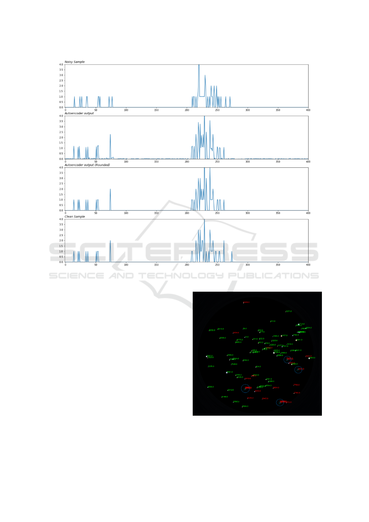
Figure 8 showcases the auto-encoders ability to

move from a noisy sample to the clean version

thereof. Displaying the discretized angular distances

of D

and D

concatenated together. The second

chart, autoencoder output, serves as the input to the

classiﬁer and is used to determine the ﬁnal prediction.

In this instance a random choice of noise and magni-

tude of that noise has been applied, resulting in minor,

but noticeable differences between the noisy sample

(top) and clean version (bottom). The auto encoder is

able to accurately move from this noisy sample to a

very close approximation of the clean sample, high-

lighted in the 3rd chart by rounding the values.

Figure 9 shows a more extreme case of noise. Us-

ing our chosen auto-encoder from the ﬁnal model we

took forward, which is stated as effective up to an

angular distance noise of 1.343

◦

, this ﬁgure shows

the results for a sample with maximum angular noise

applied. Here the deformation between the noisy

and clean sample is markedly more pronounced, and

whilst the auto-encoder output bares less resemblance

compared to our previous example, it still returns a

Noise Robustness of Data-Driven Star Classiﬁcation

181

Discretized angular distance

Count

Figure 8: Autoencoder results.

good approximation of the clean sample.

The next stage of testing is carried out using the

combined model on simulated images. Such images

contain within them a wide variation on both the noise

types and magnitude thereof. Of the 1104659 sources

classiﬁed, 1036254 of which we know to be true stars

present within the image, the model successfully clas-

siﬁes 859287 of these stars with an average conﬁ-

dence of ∼ 0.937. In contrast to (Xu et al., 2019) we

apply no ﬁnal stage of weight searching, each star is

identiﬁed solely based on its GNSs within the image.

Within the broad-strokes of results there are some key

points of note. Firstly, 68405 sources are false stars

themselves as determined by cross checking known

locations against detected source co-ordinates. Of the

149423 incorrectly identiﬁed stars, 90919 occur in

examples of extreme pixel, and thus angular, noise.

We know this by cross-checking the source location

against known stars in the image, to a certain pixel tol-

erance here set as 8 pixels. In total ∼ 13.53% of stars

are miss-identiﬁed, with ∼ 8.23% of these occurring

in instances of extreme pixel noise in the GRSs loca-

tion.

The impact of false stars and dropped stars is less

easily quantiﬁable, but by examining images we can

see that there is a much greater tendency towards

miss-identiﬁcations on the periphery of the images, as

would be expected in instances where a large portion

of the stars GNSs are cut from view, these represent

instances of signiﬁcant dropped star noise.

When considering these results through the lens of

navigation, wherein it is less necessary to identify all

stars in the image, and more important to conﬁdently

identify a select few, we can also consider what role

the conﬁdence of our model has with respect to ac-

curacy. The average conﬁdence of successful iden-

tiﬁcation is ∼ 0.94 in contrast to the conﬁdence of

∼ 0.42 in miss-identiﬁcations. By delving into these

conﬁdence scores we can examine what impact ap-

plying conﬁdence thresholds might have on identiﬁ-

cation throughout our image, the end goal being to

reduce miss-identiﬁcations, but also to eliminate as

many of the more damaging high-conﬁdence miss-

identiﬁcations as possible.

Table 3 shows how the number of correct and in-

correct identiﬁcations changes when we discard those

that do not meet a given threshold. We can see an

immediate reduction when limiting our identiﬁcations

ICPRAM 2023 - 12th International Conference on Pattern Recognition Applications and Methods

182

Discretized angular distance

Count

Figure 9: Auto-encoder results for max angular noise.

to a conﬁdence score of 0.8, we are able to discard

86.70% of incorrect identiﬁcations whilst only losing

10.33% of correct ones. At the extreme, by limit-

ing conﬁdence to 0.999 or above we lose 39.10% of

correct identiﬁcations whilst removing the vast ma-

jority, 99.85%, of incorrect identiﬁcations. This ex-

treme, presuming clear nights, would allow for cor-

rect identiﬁcation of more than enough stars for nav-

igation, whilst drastically reducing the probability of

an incorrect identiﬁcation. With additional checking

measures it would be reasonably easy to eliminate the

remaining incorrect identiﬁcations by cross checking

identiﬁcations with expected neighbouring stars in an

image.

6 CONCLUSION

In this paper we demonstrate the viability of neu-

ral network star-pattern recognition when applied to

a synthetic dataset emulating the viewpoint at the

Earths surface. The synthetic data represents a new

Figure 10: Application of model to synthetic image, correct

identiﬁcations in green and incorrect in red. Highlighted are

4 regions of false star noise due to meteor showers.

Noise Robustness of Data-Driven Star Classiﬁcation

183

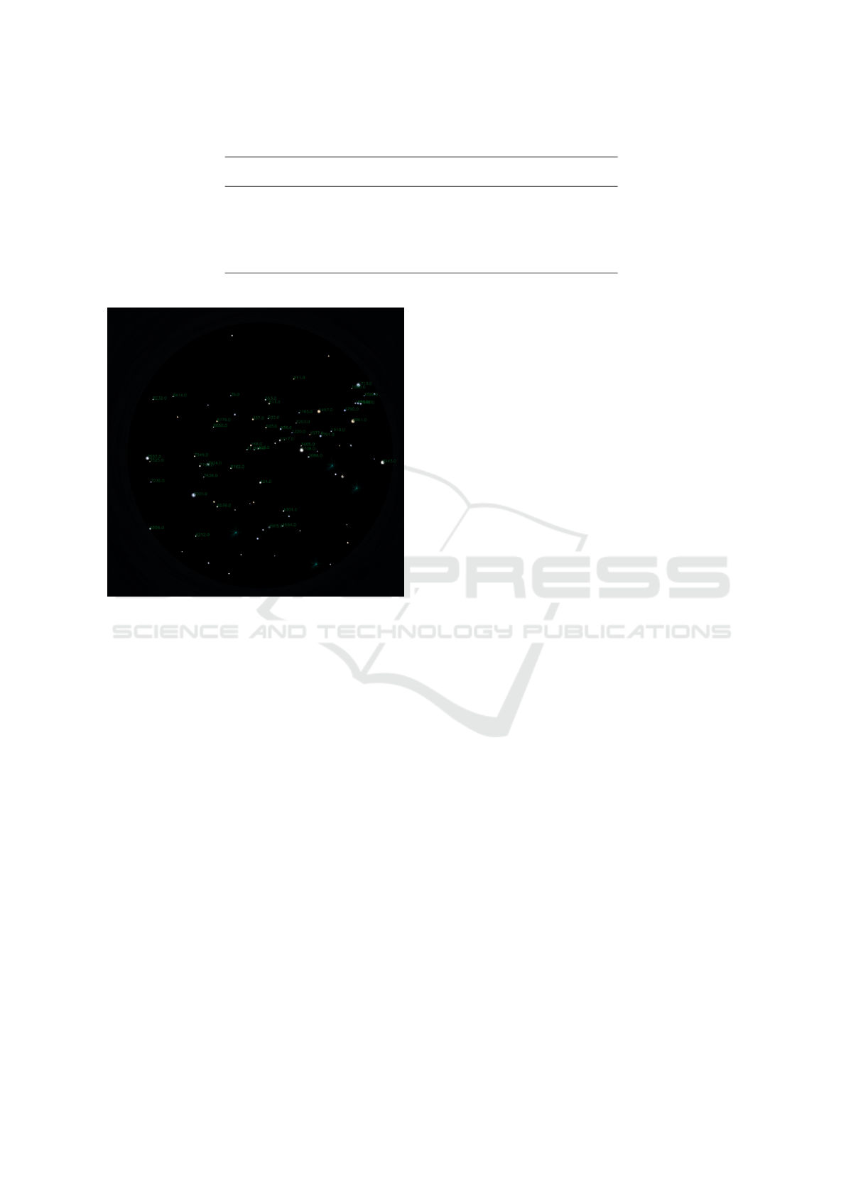
Table 3: Classiﬁcation results and thresholding impact.

Threshold

Correct

Identiﬁcations

% Change

(Total)

Incorrect

Identiﬁcations

% Change

(Total)

Baseline 859287 N/A 149423 N/A

0.8 770485 10.33% 19874 86.70%

0.9 741632 13.69% 12039 91.94%

0.95 713120 17.01% 7184 95.19%

0.99 640618 25.45% 2119 98.51%

0.999 523322 39.10% 221 99.85%

Figure 11: Synthetic image results with 0.999 conﬁ-

dence thresholding, showing the removal of all miss-

identiﬁcations in the image.

method by which we can garner realistic night-sky

images from a variety of viewpoints as well as the

corresponding information required to utilise them as

a labelled dataset of stars.

We create a data augmenter to avoid pre-

computing training patterns whilst allowing for

greater freedoms with training and testing and para-

metrically explore tolerance towards noise. The ﬁ-

nal implementation performs well on simulated star

patterns and is still able to correctly identify the ma-

jority of stars in the markedly noisier synthetic im-

ages, we threshold our images to a visible magnitude

of 3.0 in order to appropriately simulate the capabili-

ties of inexpensive cameras with low exposure times,

an important consideration when examining this tech-

nology through the lens of celestial navigation from

the Earths surface. Whilst miss-identiﬁcations do oc-

cur, we are able to drastically reduce these by utilising

conﬁdence thresholds, a necessary step if the method

were to be used for navigational purposes where miss-

identiﬁcations can be damaging.

REFERENCES

Jiang, J., Ji, F., Yan, J., Sun, L., and Wei, X. (2015).

Redundant-coded radial and neighbor star pattern

identiﬁcation algorithm. IEEE Transactions on

Aerospace and Electronic Systems, 51(4):2811–2822.

Liebe, C. (1993). Pattern recognition of star constellations

for spacecraft applications. IEEE Aerospace and Elec-

tronic Systems Magazine, 8(1):31–39.

Mortari, D., Samaan, M. A., Bruccoleri, C., and Junkins,

J. L. (2004). The pyramid star identiﬁcation tech-

nique. NAVIGATION, 51(3):171–183.

Na, M., Zheng, D., and Jia, P. (2009). Modiﬁed grid algo-

rithm for noisy all-sky autonomous star identiﬁcation.

IEEE Transactions on Aerospace and Electronic Sys-

tems, 45(2):516–522.

Nabi, A., Foitih, Z., and Mohammed El Amine, C. (2019).

Improved triangular-based star pattern recognition al-

gorithm for low-cost star trackers. Journal of King

Saud University.

Padgett, C. and Kreutz-Delgado, K. (1997). A grid al-

gorithm for autonomous star identiﬁcation. IEEE

Transactions on Aerospace and Electronic Systems,

33(1):202–213.

Rijlaarsdam, D., Yous, H., Byrne, J., Oddenino, D., Fu-

rano, G., and Moloney, D. (2020). A survey of lost-in-

space star identiﬁcation algorithms since 2009. Sen-

sors, 20(9).

Stetson, P. B. (1987). DAOPHOT: A Computer Program

for Crowded-Field Stellar Photometry. Publications

of the Astronomical Society of the Paciﬁc, 99:191.

van Bezooijen, R. (1989). A star pattern recognition al-

gorithm for autonomous attitude determination. IFAC

Proceedings Volumes, 22(7):51–58. IFAC Symposium

on Automatic Control in Aerospace, Tsukuba, Japan,

17-21 July 1989.

Wang, G., Li, J., and Wei, X. (2018). Star identiﬁca-

tion based on hash map. IEEE Sensors Journal,

18(4):1591–1599.

Xu, L., Jiang, J., and Liu, L. (2019). Rpnet: A representa-

tion learning based star identiﬁcation algorithm. IEEE

Access, PP:1–1.

Yang, S., Liu, L., Zhou, J., Zhao, Y., Hua, G., Sun, H.,

and Zheng, N. (2022). Robust and efﬁcient star iden-

tiﬁcation algorithm based on 1-d convolutional neural

network. IEEE Transactions on Aerospace and Elec-

tronic Systems, 58(5):4156–4167.

Zhang, G., Wei, X., and Jiang, J. (2008). Full-sky au-

tonomous star identiﬁcation based on radial and cyclic

features of star pattern. Image and Vision Computing,

26(7):891–897.

ICPRAM 2023 - 12th International Conference on Pattern Recognition Applications and Methods

184