On Converting Logic Programs Into Matrices
Tuan Nguyen Quoc
a
and Katsumi Inoue
b
National Institute of Informatics, Tokyo, Japan
Keywords:
Logic Programming, Linear Algebra, Matrix Representation.
Abstract:
Recently it has been demonstrated that deductive and abductive reasoning can be performed by exploiting the
linear algebraic characterization of logic programs. Those experimental results reported so far on both forms
of reasoning have proved that the linear algebraic approach can reach higher scalability than symbol manip-
ulations. The main idea behind these proposed algorithms is based on linear algebra matrix multiplication.
However, it has not been discussed in detail yet how to generate the matrix representation from a logic pro-
gram in an efficient way. As conversion time and resulting matrix dimension are important factors that affect
algebraic methods, it is worth investigating in standardization and matrix constructing steps. With the goal
to strengthen the foundation of linear algebraic computation of logic programs, in this paper, we will clarify
these steps and propose an efficient algorithm with empirical verification.
1 INTRODUCTION
Recently, Logic Programming (LP), which provides
languages for declarative problem solving and sym-
bolic reasoning (Lloyd, 2012), has started gaining
more attention in terms of building explainable learn-
ing models (Shakerin and Gupta, 2020; D’Asaro
et al., 2020; Garcez and Lamb, 2020; Hitzler, 2022).
For decades, LP representation has been consid-
ered mainly in the form of symbolic logic (Kowal-
ski, 1979), which is useful for declarative problem-
solving and symbolic reasoning. Since then, re-
searchers have developed various dedicated solvers
and efficient tools for Answer Set Programming
(ASP) - LP that are based on the stable model se-
mantics (Schaub and Woltran, 2018). On the other
hand, many researchers attempt to translate logical in-
ference into numerical computation in the context of
mixed integer programming (Bell et al., 1994; Gor-
don et al., 2009; Hooker, 1988; Liu et al., 2012).
They exploit connections between logical inference
and mathematical computation that open a new way
for efficient implementations.
Lately, several studies have been done on embed-
ding logic programs to numerical spaces and exploit-
ing algebraic characteristics (Sakama et al., 2017;
Sato, 2017; Aspis et al., 2020). There are multi-
ple reasons for considering linear algebraic compu-
a
https://orcid.org/0000-0002-1754-9329
b
https://orcid.org/0000-0002-2717-9122
tation of LP. First, linear algebra is at the heart of
a myriad of applications of scientific computation,
and integrating linear algebraic computation and sym-
bolic computation is considered a challenging topic
in Artificial Intelligence (AI) (Saraswat, 2016). In
particular, transforming symbolic representations into
vector spaces and reasoning through matrix compu-
tation are considered one of the most promising ap-
proaches in neural-symbolic integration (Garcez and
Lamb, 2020). Second, linear algebraic computation
has the potential to develop scalable techniques deal-
ing with huge relational knowledge bases that have
been reported in several studies (Nickel et al., 2015;
Rockt
¨
aschel et al., 2014; Yang et al., 2015). Since
relational KBs consist of ground atoms, the next chal-
lenge is applying linear algebraic techniques to LP
and deductive Knowledge Base (KB)s. Third, it
would enable us to use efficient (parallel) algorithms
of numerical linear algebra for computing LP, and
further simplify the core method so that one can ex-
ploit great computing resources ranging from multi-
threaded CPU to GPU. The promising efficiency has
been reported in GraphBLAS where various graph al-
gorithms are redefined in the language of linear alge-
bra (Davis, 2019).
(Sakama et al., 2017) has coined the linear char-
acteristics of the logic program by realizing deduc-
tive reasoning using matrix multiplication. The main
idea is to transform a logic program into a matrix and
then perform the T
P
-operator (van Emden and Kowal-
Quoc, T. and Inoue, K.
On Converting Logic Programs Into Matrices.
DOI: 10.5220/0011802400003393
In Proceedings of the 15th International Conference on Agents and Artificial Intelligence (ICAART 2023) - Volume 2, pages 405-415
ISBN: 978-989-758-623-1; ISSN: 2184-433X
Copyright
c
 2023 by SCITEPRESS – Science and Technology Publications, Lda. Under CC license (CC BY-NC-ND 4.0)
405

ski, 1976) in vector spaces by matrix multiplication
(Sakama et al., 2017). Further extensions to disjunc-
tive logic programs and normal logic programs are
also discussed later in (Sakama et al., 2021). Based
on these works, linear algebraic approaches have been
developed for deduction (Nguyen et al., 2022) and
abduction (Nguyen et al., 2021b) with great poten-
tial for scalability. Both the methods for deduction
and abduction share the same way to convert a logic
program into a matrix. This step is very important
because it affects the execution time remarkably and
also the dimension of the standardized matrix for fur-
ther reasoning steps. However, the conversion step is
not yet discussed in detail, therefore, in this paper, we
conduct a detailed analysis of it and also propose an
efficient algorithm to convert a logic program into a
matrix with the goal to strengthen the foundation of
linear algebraic computation of logic programs.
The rest of this paper is organized as follows: Sec-
tion 2 describes the preliminaries and the definitions
of program matrix for definite and normal logic pro-
grams; Section 3 analyzes the method in detail fo-
cusing on time complexity and also proposes a lin-
ear complexity algorithm to deal with converting a
logic program into a matrix; Section 4 demonstrates
the proposed algorithm on the graph coloring problem
and verifies it has linear complexity; Section 5 dis-
cusses different matrix representation using by other
linear algebraic methods in LP; Section 6 gives con-
clusion and discusses future work.
2 MATRIX REPRESENTATION
OF LOGIC PROGRAM
The linear algebraic characteristics of LP were first
analyzed by (Sakama et al., 2017; Sakama et al.,
2021). We hereafter mention again the matrix rep-
resentation of the logic program.
We consider a language L that contains a finite
set of propositional variables. A logic program P is a
finite set of clauses defined over a number of alpha-
bets and the logical connectives ¬, ∧, ∨, and ←. The
Herbrand base B
P
is the set of all propositional vari-
ables in a logic program P. A rule in P can be in one
of the forms (1), (2), or (3).
h ← b
1
∧ b
2
∧ ... ∧ b
l
(l ≥ 0) (1)
h ← b
1
∨ b
2
∨ ... ∨ b
l
(l ≥ 0) (2)
h ← b
1
∧ b
2
∧ ... ∧ b
l
∧ ¬b
l+1
∧ ... ∧ ¬b
l+k
(3)
(l + k ≥ l ≥ 0)
where h and b
i
are propositional variables in L .
For convenience, we refer to (1) as an And-rule, (2) as
an Or-rule, and (2) as a normal rule.
For each rule r of the form (1) or (2) we de-
fine head(r) = h and body(r) = {b
1
, ..., b
l
}. For
each normal rule r (3), we define head(r) = h and
body(r) = {b
1
, ..., b
l
, ¬b
l+1
, ..., ¬b
l+k
}. Its body(r)
is partitioned into body
+
(r) = {b
1
, b
2
, ..., b
l
} and
body
−
(r) = {¬b
l+1
, ¬b
l+2
, ..., ¬b
l+k
} which refers
to the positive and negative occurrences of atoms in
body(r), respectively. A rule r is a fact if body(r) =
/
0.
A rule r is a constraint if head(r) =
/
0. A rule r is in-
valid if both head(r) and body(r) are
/
0.
A definite program is a finite set of And-rules (1)
or Or-rules (2). Note that an Or-rule is a shorthand
of l And-rule h ← b
1
, h ← b
2
, ... h ← b
l
. A def-
inite program P is called an Singly-Defined (SD)-
program if there are no two rules with the same
head in it. Every definite program can be con-
verted into an SD-program in the following manner.
If there is more than one rule with the same head
{h ← body(r
1
), ..., h ← body(r
j
)}, where j > 1 and
body(r
1
), ..., body(r
j
) 6=
/
0 (or h is not a f act). One
can replace them with a set of rules {h ← b
1
∨ ... ∨
b
j
, b
1
← body(r
1
), ..., b
j
← body(r
j
)} including an
Or-rule and j And-rules for j newly introduced atoms
{b
1
, ..., b
j
}. We refer to the converted SD-program
of a definite program P as a standardized program P
δ
.
A normal program is a finite set of rules of the
form (3). Note that a normal program P is a definite
program if body
−
(r) =
/
0 for every rule r ∈ P. Nor-
mal logic programs can be transformed into definite
programs as mentioned in (Alferes et al., 2000). Ac-
cordingly, one can obtain a definite program from a
normal program P by replacing the negated literals in
every rule of the form (3) and rewriting as follows:
h ← b
1
∧ b
2
∧ ... ∧ b
l
∧ b
l+1
∧ ... ∧ b
l+k
(4)
(l + k ≥ l ≥ 0)
where each b
i
is the positive form of the negation ¬b
i
.
The resulting program is called the positive form of
P, denote as P
+
. In terms of model computation, the
stable models of P can be computed from the least
model of P
+
and interpretation vectors as proposed in
(Sakama et al., 2017; Sakama et al., 2021; Takemura
and Inoue, 2022).
For convenience, we also adopt the definition of
the same head logic program (SHLP) in (Gao et al.,
2022) to the propositional language. In our paper, an
SHLP is a normal logic program such that it has at
least two rules of the same head. A normal program P
may contain multiple SHLPs in it. This definition will
be used in the next section for complexity analysis.
The main idea of representing a logic program us-
ing a matrix is to create a mapping from the set of all
atoms to row/column indices of the matrix. It is es-
sential for a matrix representation of a logic program
ICAART 2023 - 15th International Conference on Agents and Artificial Intelligence
406

to contain exactly one row and one column for each
atom in a program matrix. That is why we need to
consider a program P in the standardized format. One
can find a bijection from its set of atoms to indices of
a matrix to represent every rule of P as a row in the
matrix as follows:
Definition 1. Matrix Representation of Standard-
ized Programs: (Sakama et al., 2021) Let P be a
standardized program and B
P
= {p
1
, . . ., p
n
}. Then
P is represented by a matrix M
P
∈ R
n×n
such that for
each element a
i j
(1 ≤ i, j ≤ n) in M
P
,
1. a
i j
k
=
1
l
(1 ≤ k ≤ l; 1 ≤ i, j
k
≤ n) if p
i
← p
j
1
∧
··· ∧ p
j
l
is in P;
2. a
i j
k
= 1 (1 ≤ k ≤ c; 1 ≤ i, j
k
≤ n) if p
i
← p
j
1
∨
··· ∨ p
j
c
is in P;
3. a
ii
= 1 if p
i
← is in P;
4. a
i j
= 0, otherwise.
M
P
is called a program matrix of P. Let us consider
a concrete example for a better understanding of Def-
inition 1:
Example 1. Consider a definite program P = {p ←
q ∧ r, p ← q ∧ s, q ← t, q ← s ∧ u, r ←, s ←}.
P is not an SD program because p ← q ∧ r, p ← q ∧ s
have the same head p and q ← t, q ← s ∧ u have
the same head q. Then P is converted into the
standardized program P
δ
by introducing new atoms
x
1
= q ∧ r, x
2
= q ∧ s and x
3
= s ∧ u as follows:
P
δ
= {p ← x
1
∨ x
2
, q ← t ∨ x
3
, r ←, s ←, x
1
←
q ∧ r, x
2
← q ∧ s, x
3
← s ∧ u}. Then by applying
Definition 1, one can obtain
1
:












p q r s t u x
1
x
2
x
3
p 1.00 1.00
q 1.00 1.00
r 1.00
s 1.00
t
u
x
1
0.50 0.50
x
2
0.50 0.50
x
3
0.50 0.50












Note that it is not needed to introduce a new atom
for the single-length body rule q ← t. Additionally,
an introduced body can also be reused immediately
without re-introducing it twice.
As mentioned, we have a way to transform normal
logic programs into standardized programs, therefore
representing a normal program P is made easy by first
transforming it into a positive form P
+
and then con-
verting P
+
into a standardized program P
+
.
1
We omit all zero elements in matrices for better read-
ability.
Definition 2. Matrix Representation of Normal
Programs: (Sakama et al., 2021) Let P be a
normal program, and P
+
its transformed posi-
tive form as a standardized program. Suppose
that the Herbrand base of P
+
is given by B
P
+
=
{p
1
, . . . , p
n
, q
n+1
, . . . , q
n+k
} where p
i
are positive
literals and q
j
(n + 1 ≤ j ≤ n + k) are negative literals
appearing in P
+
. Then P
+
is represented by a ma-
trix M
P
+
∈ R
(n+k)×(n+k)
such that for each element
a
i j
(1 ≤ i, j ≤ n + k) in P
+
:
1. a
ii
= 1 for n + 1 ≤ i ≤ n + k;
2. a
i j
= 0 for n + 1 ≤ i ≤ n + k and 1 ≤ j ≤ n + k
such that i 6= j;
3. Otherwise, a
i j
(1 ≤ i ≤ n; 1 ≤ j ≤ n + k) is en-
coded as in Definition 1.
Let us consider an example.
Example 2. Consider a normal program
P = {p ← q ∧ ¬r, q ← r ∧ ¬p, r ← p ∧ ¬q}.
First, transform P to P
+
such that P
+
= {p ←
q ∧ r, q ← r ∧ p, r ← p ∧ q}. P
+
satisfies the SD
condition, therefore, its transformed positive form as
a standardized program P
+
= P
+
. Then by applying
Definition 2, one can obtain:







p q r p q r
p 0.50 0.50
q 0.50 0.50
r 0.50 0.50
p 1.00
q 1.00
r 1.00







3 LOGIC PROGRAM TO MATRIX
CONVERSION
According to the previous section, we can have a
quick summary of the logic program to matrix con-
version method as described in Figure 1. In this sec-
tion, we focus on the time complexity of the algebraic
method. First, let us assume a logic program P with
|B
P
| = n. Let m be the number of rules in P, l be the
average length of rules in P, k (k ≤ n) the number of
negations appearing in P, g be the number of SHLPs
in P, and l
g
is the average number of rules in each
SHLP of P.
Converting to Positive Form.
First, one has to scan the whole program to identify
all negations in P. Thus, the complexity of this step
is Θ(ml). Additionally, the resulting program P
+
of
On Converting Logic Programs Into Matrices
407

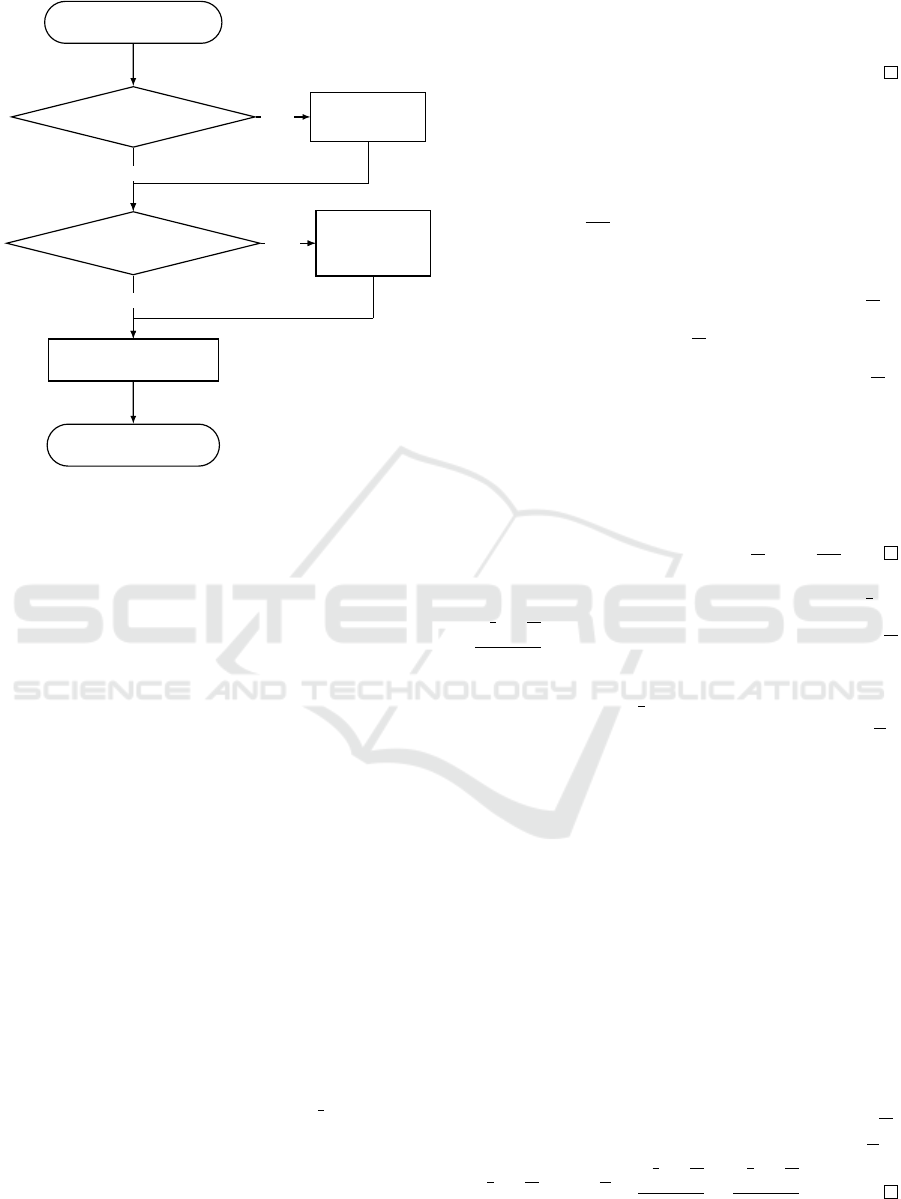
START with a logic program P
Is P a normal program?
1. Convert P to a
positive form P
+
P := P
+
Is P standardized?
2. Convert P to
a standardized
program P
δ
P := P
δ
3. Convert P into a matrix M
P
RETURN program matrix M
P
True
False
False
True
Figure 1: The flow of the logic program to matrix conver-
sion method.
this step has more atoms than P has. In fact, we intro-
duce new positive forms for all negations appearing
in P, therefore |B
P
+
| = n + k. This is also the number
of atoms in the positive form program P
+
. One can
take the normal program in Example 2 to verify the
calculation.
Converting to Standardized Program.
In the standardization step, we have to introduce a
new Or-rule for each SHLP as mentioned in the pre-
vious section. In order to do that, first, we need a
way to identify all SHLPs in P. Next, for each SHLP,
we introduce a new atom for all the rule bodies with
more than 1 atom in those. Then for that SHLP, we
introduce a new Or-rule which includes all newly in-
troduced atoms and all rule bodies of the length 1.
Because the number of rules of P is m, which does
not change through the step converting to the positive
form, the maximum number of new atoms we need to
introduce is m. The worst case happens when all rule
bodies are unique with length > 1 and they all belong
to one of the SHLPs.
Let P
0
be the obtained program of P after the stan-
dardization step. Accordingly, n
0
is the number of
atoms, m
0
is the number of rules, and l
0
is the aver-
age rule length. The following proposition holds:
Proposition 1. The number of atoms of P
0
, n
0
, is
bounded by n + m + k.
Proof. According to the mentioned explanations
above for each conversion step, we have to intro-
duce exactly k new positive forms for all negations
and at most m new atoms for all SHLPs. Hence,
n
0
≤ n + m + k.
The number of rules m
0
of P
0
is also increased as
we have to introduce new rules for each SHLP. The
following proposition holds:
Proposition 2. The number of rules of P
0
, m
0
, is
bounded by

3m
2

.
Proof. As defined, an SHLP must have at least two
rules, so the largest number of SHLPs in P is
j
m
2
k
.
It happens when we have
j
m
2
k
pairs of rules with the
same head. In this case, we need to introduce
j
m
2
k
new Or-rules for each pair. Additionally, if we as-
sume all the rule bodies are unique and have a length
larger than 1, we have to introduce m new atoms for
those bodies to create new corresponding And-rules.
These new And-rules will replace the old same head
rules, so the number of And-rules remains the same.
Therefore, m
0
is bounded by m +
j
m
2
k
=

3m
2

.
Proposition 3. The average rule length of P
0
is l
0
=
ml + gl
g
m + g
, where g > 0 is the number of SHLPs and l
g
is the average number of rules in each SHLP.
Proof. Obviously, ml is the total length of all rules in
P. Similarly, the total length of all rules in P
0
is m
0
l
0
.
Now consider the case there is an SHLP having
two rules: h ← body(r
1
) and h ← body(r
2
). In
this case, the number of SHLPs g = 1. The stan-
dardization step will replace these two rules by
{h ← x
1
∨ x
2
, x
1
← body(r
1
), x
2
← body(r
2
)}. As
one can see, only the new disjunction h ← x
1
∨ x
2
affects the average rule length of P
0
. A similar
manner can be extended to different SHLPs in P.
Accordingly, we only need to determine how many
of these rules will be introduced and the total length
of them in P
0
.
Because we need to introduce a new disjunction
rule for each SHLP, we have the number of rules m
0
=
m + g. Additionally, the body length of a disjunction
for each SHLP is also equal to the number of rules
in that SHLP. So the increasing length of P
0
is gl
g
.
Therefore, the total length of every rule in P
0
is m
0
l
0
=
ml + gl
g
. Thus, l
0
=
ml + gl
g
m
0
=
ml + gl
g
m + g
.
ICAART 2023 - 15th International Conference on Agents and Artificial Intelligence
408

Corollary 1. The average rule length l
0
is bounded:
l
0
≤
ml + m
m + 1
Proof. According to the proof of Proposition 3, the
increasing length of P
0
after introducing new disjunc-
tions is m
0
l
0
= ml + gl
g
. Because P has maximum m
rules, the total body length of newly introduced dis-
junctions cannot exceed m. Consequently, gl
g
≤ m ⇒
l
0
≤
ml + m
m + g
≤
ml + m
m + 1
. Equality happens when all
rule bodies of P belong to an SHLP.
Converting to Program Matrix.
Combining Proposition 1 and Definition 1, we have
the following proposition:
Proposition 4. The lower bound of the dimension of
the program matrix M
P
is n× n while the upper bound
is (n + m + k) × (n + m + k).
Proof. The lower bound is explained in the first step
converting to the positive form, therefore, we only
need to prove the upper bound. According to Propo-
sition 1, the upper bound of the dimension of the pro-
gram matrix is (n + m + k) × (n + m + k). Hence,
the dimension of the program matrix is bounded by
(n + m + k) × (n + m + k).
On the other hand, the number of negations is
bounded by the number of atoms in P or k ≤ n, so
we can also write that the dimension of the program
matrix is bounded by (2n + m) × (2n + m).
The next step is converting P
0
into a matrix. In this
step, we first init a zero matrix of the size n
0
×n
0
. Then
we go through all rules in P
0
to assign a value for each
atom that appears in the rule body by a value follow-
ing Definition 1. The following proposition holds:
Proposition 5. The number of needed assignments to
convert P
0
into a matrix is bounded by ml + m
Proof. Based on Definition 1, the number of needed
assignments is m
0
l
0
, where m
0
is the number of rules
and l
0
is the average rule length of P
0
. According to
Proposition 3, l
0
=
ml + gl
g
m + g
and m
0
= m + g, there-
fore, m
0
l
0
= ml + gl
g
. As already mentioned in the
proof of Corollary 1, we have gl
g
≤ m. Accordingly,
m
0
l
0
≤ ml + m.
In summary, we need at most ml + m assignments in
converting a logic program P into a matrix of the size
which is bounded by (n + m + k) × (n + m + k).
Now, we will discuss how to implement the
method efficiently. Through what we have analyzed
above, the key is to avoid introducing new atoms if
not needed and optimize the number of assignments
as much as possible. An efficient way to implement
this method is by exploiting a hashtable data structure
for storing rules. For each item in the hashtable, key
is the head of a rule and value is an array of rule bod-
ies. A fact is an item with the value as an empty array.
The hashtable ensures the complexity of look up and
insertion of a key-value pair is O(1) in average. The
detailed method of converting a logic program into a
matrix is described in Algorithm 1.
Algorithm 1: Converting a standardized program into a ma-
trix.
Input: A logic program P
Output: Matrix representation M
P
0
of P
0
where P
0
is
the standardized program obtained from P
1: Init H := {
/
0}.  Hashtable
2: for each rule r in P do
3: for each atom b in body of r do
4: if b is negation then
5: Introduce positive form b of b.
6: Insert b into H .  empty-body rule
7: if head of r is not in H then
8: Insert r into H .
9: else
10: Append body of r to value of the existing
item of r in H .
11: for each r in H that has more than 1 body do
12: for each body b of the rule r do
13: if |b| > 1 then
14: Introduce a new atom for b.
15: Insert this new And-rule into H .
16: Clear the all rule bodies in the value of r and
update r to Or-rule with newly introduced atoms.
17: n
0
= sizeof(H ).
18: Create a zero matrix M
P
0
of the size R
n
0
×n
0
.
19: for each rule r in H do
20: Assigning M
P
0
according to Definition 1.
21: return assigned matrix M
P
0
.
On Converting Logic Programs Into Matrices
409

Some explanations are in order:
• Step 2-10: Scan through all rules in the program
and convert all negations to positive forms. Up-
date the hashtable H by either inserting a new rule
or updating the rule body of an existing rule. The
complexity of this step is O(ml) because we need
to go through all the rules in the logic program P
and for each rule, we also need to verify whether
it contains negation or not.
• Step 11-16: Loop over only SHLPs and do the
standardization step. In case all rules of P belong
to an SHLP, we have to scan all these rules in P to
introduce new atoms for each rule body as in the
standardization step. Accordingly, the complexity
of this step is O(m).
• Step 19-20: Assigning values to the matrix ac-
cording to Definition 1. According to Proposi-
tion 5, the number of needed assignments to con-
vert P
0
into a matrix is bounded by m
l + m. This is
also the number of non-zero elements in the out-
put matrix. Therefore, the complexity of this step
is O(ml + m).
As a result, the time complexity of Algorithm 1 is
O

ml + m + m(l + 1)

= O

2ml + 2m

= O

ml

,
in other words, linear to the number of rules in P
if we consider l as a constant. A similar result can
be extended to the abductive matrix as it is defined
based on the program matrix (Nguyen et al., 2021b).
The time complexity of Algorithm 1 is indepen-
dent of the matrix representation format. It is worth
noting that in the standardization step, introducing a
new atom for a body of length 1 is not needed.
Proposition 6. Any algorithm converting a logic pro-
gram into a matrix has the lower bound Ω(ml).
Proof. Any algorithm converting a logic program into
a matrix has to go through all the rules of P at least
once to read these rules into memory. Therefore, no
algorithm can do better than Ω(ml).
To sum up, we have proposed Algorithm 1, which
has linear complexity, for the problem of converting
a logic program into a matrix. In Section 4, we will
provide an experiment to verify this conclusion.
4 BASELINE EXPERIMENT
For the purpose of this work, we provide a base-
line experiment to verify the time complexity of the
method of converting logic programs into matrices.
Experiment Setup.
In this experiment, we use the graph coloring prob-
lem - a problem in graph theory in that we search
for possible a way of coloring all the vertices of
a graph such that no pair of adjacent vertices are
of the same color. The graph coloring problem
can be formulated in first-order logic as follows:
Listing 1: Modeling of graph coloring in ASP language.
1color ( 1 . . 3 ) .
21 { n ode_co l o r ( N , C ) : c o lor ( C ) } 1 : -
node ( N) .
3: - n o d e _color (X ,C ) , n o d e _ color (Y ,C ) ,
edge ( X , Y ) , c o lor ( C ) .
This example is written following the syntax of an
ASP language specified by clingo solver (clasp)
(Gebser et al., 2009). In Listing 1, the first line
defines there are 3 colors we can use to label nodes
(3-Coloring). The second line is a choice rule that
defines a node that can be labeled by only one
color. And finally, the third rule is a constraint that
declares there are no two adjacent nodes that can be
labeled with the same color. Listing 2 illustrates an
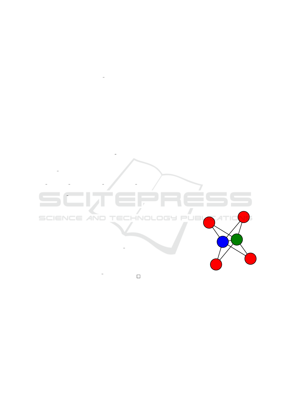
instance of the graph coloring problem with 6 nodes.
Listing 2: A problem
instance of the graph
coloring problem.
1node ( n1 ) .
2node ( n2 ) .
3node ( n3 ) .
4node ( n4 ) .
5node ( n5 ) .
6node ( n6 ) .
7edge ( n1 , n2 ) .
8edge ( n1 , n3 ) .
9edge ( n2 , n3 ) .
10edge ( n1 , n4 ) .
11edge ( n2 , n4 ) .
12edge ( n1 , n5 ) .
13edge ( n2 , n5 ) .
14edge ( n1 , n6 ) .
15edge ( n2 , n6 ) .
n1
n2
n3
n4
n5
n6
Figure 2.
We exploit clingo grounder (gringo) (Gebser
et al., 2007) to deal with ASP format. First, clingo
converts an ASP program into an ASP intermediate
format - aspif (Gebser et al., 2016). In short, a pro-
gram in an ASP intermediate format serves internally
as the output of the grounder and the input of the
solver. We then convert the obtained aspif format into
our internal format which is equivalent to a proposi-
tional language as described in Section 2. The result-
ing program now can be treated as an input for Al-
gorithm 1 to obtain the matrix representation. It is
reported that the program matrix is highly sparse if
the average rule length is small compared to the size
ICAART 2023 - 15th International Conference on Agents and Artificial Intelligence
410

Table 1: Baseline results on the graph coloring problem (the unit of time is millisecond).
No. Data instance (70 instances) m n k m
0
n
0
l η
z
t
clingo
t
int
t
alg
t
(d)
asg
t
(s)
asg
1 01 octahedral.txt 105 63 30 106 136 1.981 267 0.330 0.027 0.273 0.068 0.147
2 02 33fan.txt 101 62 30 102 132 1.971 257 0.312 0.025 0.281 0.065 0.145
3 03 42fan.txt 93 60 30 94 124 1.947 237 0.244 0.023 0.212 0.035 0.135
4 04 K133.txt 126 74 35 127 162 2.000 321 0.266 0.026 0.277 0.067 0.153
5 05 43cone.txt 130 75 35 131 166 2.008 331 0.260 0.027 0.288 0.091 0.156
6 06 43fan.txt 122 73 35 123 158 1.992 311 0.254 0.026 0.267 0.045 0.158
7 07 52fan.txt 110 70 35 111 146 1.964 281 0.249 0.025 0.247 0.041 0.146
8 08 K134.txt 151 86 40 152 192 2.020 385 0.287 0.033 0.338 0.087 0.174
9 g500a.txt 30,983 10,623 2,500 30,984 33,484 2.197 78,203 164.252 12.064 75.842 46.138 21.731
10 g500b.txt 31,215 10,681 2,500 31,216 33,716 2.198 78,783 161.577 12.641 79.654 46.807 21.747
11 g500c.txt 31,159 10,667 2,500 31,160 33,660 2.198 78,643 167.144 12.839 94.754 46.899 22.856
12 g500d.txt 30,631 10,535 2,500 30,632 33,132 2.197 77,323 162.624 12.772 98.012 48.870 22.276
13 g500e.txt 31,247 10,689 2,500 31,248 33,748 2.198 78,863 166.513 13.261 117.535 47.481 22.746
14 g1000a.txt 62,259 21,317 5,000 62,260 67,260 2.198 157,143 603.443 11.494 192.126 NA 39.980
15 g1000b.txt 61,523 21,133 5,000 61,524 66,524 2.197 155,303 519.572 10.429 184.788 96.685 39.284
16 g1000c.txt 63,059 21,517 5,000 63,060 68,060 2.198 159,143 510.697 10.153 209.855 NA 40.232
17 g1000d.txt 61,411 21,105 5,000 61,412 66,412 2.197 155,023 505.066 9.622 186.825 97.017 39.611
18 g1000e.txt 62,811 21,455 5,000 62,812 67,812 2.198 158,523 517.933 9.911 213.331 NA 40.649
19 g1500a.txt 132,823 41,833 7,500 132,824 140,324 2.213 334,303 1,464.692 24.899 487.264 NA 85.393
20 g1500b.txt 132,119 41,657 7,500 132,120 139,620 2.213 332,543 1,369.828 23.139 464.427 NA 101.596
21 g1500c.txt 134,519 42,257 7,500 134,520 142,020 2.214 338,543 1,365.100 23.323 491.663 NA 87.459
22 g1500d.txt 132,255 41,691 7,500 132,256 139,756 2.213 332,883 1,380.001 22.866 449.122 NA 89.254
23 g1500e.txt 133,887 42,099 7,500 133,888 141,388 2.214 336,963 1,369.460 23.022 479.502 NA 87.569
24 g2000a.txt 229,491 68,875 10,000 229,492 239,492 2.222 576,723 2,831.258 43.639 856.753 NA 152.884
25 g2000b.txt 229,763 68,943 10,000 229,764 239,764 2.222 577,403 2,565.067 41.061 887.015 NA 152.745
26 g2000c.txt 231,147 69,289 10,000 231,148 241,148 2.222 580,863 2,579.886 42.584 819.382 NA 153.804
27 g2000d.txt 231,707 69,429 10,000 231,708 241,708 2.222 582,263 2,572.219 40.758 908.208 NA 156.532
28 g2000e.txt 230,411 69,105 10,000 230,412 240,412 2.222 579,023 2,517.911 41.468 840.034 NA 157.877
29 g2500a.txt 353,639 102,787 12,500 353,640 366,140 2.227 887,843 4,477.236 71.675 1,433.340 NA 242.757
30 g2500b.txt 354,639 103,037 12,500 354,640 367,140 2.227 890,343 4,427.957 68.898 1,375.676 NA 247.986
31 g2500c.txt 353,999 102,877 12,500 354,000 366,500 2.227 888,743 4,478.155 65.696 1,362.169 NA 244.847
32 g2500d.txt 356,127 103,409 12,500 356,128 368,628 2.227 894,063 4,400.563 67.971 1,331.527 NA 248.394
33 g2500e.txt 355,415 103,231 12,500 355,416 367,916 2.227 892,283 4,455.153 70.469 1,410.733 NA 245.272
34 g3000a.txt 384,979 113,497 15,000 384,980 399,980 2.225 966,943 6,649.247 79.231 1,525.205 NA 265.820
35 g3000b.txt 386,771 113,945 15,000 386,772 401,772 2.225 971,423 6,125.425 75.262 1,478.556 NA 266.498
36 g3000c.txt 385,899 113,727 15,000 385,900 400,900 2.225 969,243 6,078.847 75.971 1,554.599 NA 267.996
37 g3000d.txt 386,843 113,963 15,000 386,844 401,844 2.225 971,603 6,030.022 73.548 1,450.245 NA 266.121
38 g3000e.txt 387,595 114,151 15,000 387,596 402,596 2.225 973,483 6,039.618 77.444 1,560.791 NA 268.629
39 g3500a.txt 422,263 125,693 17,500 422,264 439,764 2.223 1,060,903 8,833.187 87.178 1,530.809 NA 292.929
40 g3500b.txt 422,487 125,749 17,500 422,488 439,988 2.223 1,061,463 8,812.472 91.360 1,758.592 NA 301.646
41 g3500c.txt 422,111 125,655 17,500 422,112 439,612 2.223 1,060,523 9,003.760 88.826 1,719.789 NA 297.962
42 g3500d.txt 425,415 126,481 17,500 425,416 442,916 2.223 1,068,783 8,440.211 82.093 1,625.366 NA 295.812
43 g3500e.txt 424,951 126,365 17,500 424,952 442,452 2.223 1,067,623 8,506.824 81.822 1,668.312 NA 296.487
44 g4000a.txt 545,851 159,465 20,000 545,852 565,852 2.226 1,370,623 11,829.531 114.623 2,149.171 NA 379.328
45 g4000b.txt 547,731 159,935 20,000 547,732 567,732 2.226 1,375,323 10,600.458 118.387 2,185.071 NA 381.556
46 g4000c.txt 546,939 159,737 20,000 546,940 566,940 2.226 1,373,343 10,575.754 108.357 2,225.634 NA 378.562
47 g4000d.txt 550,507 160,629 20,000 550,508 570,508 2.226 1,382,263 10,460.095 107.292 2,128.184 NA 381.873
48 g4000e.txt 550,307 160,579 20,000 550,308 570,308 2.226 1,381,763 10,656.230 108.578 2,083.164 NA 381.546
49 g4500a.txt 580,591 171,025 22,500 580,592 603,092 2.225 1,458,223 14,352.234 124.617 2,290.720 NA 409.873
50 g4500b.txt 579,287 170,699 22,500 579,288 601,788 2.225 1,454,963 13,937.675 124.642 2,321.257 NA 404.875
51 g4500c.txt 580,343 170,963 22,500 580,344 602,844 2.225 1,457,603 13,930.808 126.757 2,271.633 NA 403.584
52 g4500d.txt 581,143 171,163 22,500 581,144 603,644 2.225 1,459,603 13,842.388 127.051 2,237.434 NA 406.271
53 g4500e.txt 584,407 171,979 22,500 584,408 606,908 2.225 1,467,763 14,125.477 129.132 2,290.216 NA 409.394
54 g5000a.txt 711,547 206,639 25,000 711,548 736,548 2.227 1,786,363 18,390.131 152.617 2,828.521 NA 496.992
55 g5000b.txt 712,211 206,805 25,000 712,212 737,212 2.227 1,788,023 18,301.363 158.893 2,785.979 NA 510.082
56 g5000c.txt 713,467 207,119 25,000 713,468 738,468 2.227 1,791,163 18,218.742 155.108 2,890.195 NA 509.008
57 g5000d.txt 712,851 206,965 25,000 712,852 737,852 2.227 1,789,623 18,273.827 143.145 2,828.261 NA 503.874
58 g5000e.txt 716,187 207,799 25,000 716,188 741,188 2.227 1,797,963 18,455.484 149.504 2,725.695 NA 502.417
59 structured-type1-100nodes.txt 2,991 1,325 500 2,992 3,492 2.138 7,623 9.821 1.090 6.781 3.928 1.957
60 structured-type1-900nodes.txt 28,751 12,365 4,500 28,752 33,252 2.148 73,223 606.712 13.673 72.614 43.158 20.259
61 structured-type1-1600nodes.txt 51,531 22,085 8,000 51,532 59,532 2.149 131,223 1,693.839 19.363 160.946 80.609 37.406
62 structured-type1-2500nodes.txt 80,911 34,605 12,500 80,912 93,412 2.149 206,023 3,951.911 26.385 289.428 NA 59.276
63 structured-type1-3600nodes.txt 116,891 49,925 18,000 116,892 134,892 2.150 297,623 8,187.798 33.079 467.196 NA 83.547
64 structured-type1-400nodes.txt 12,571 5,445 2,000 12,572 14,572 2.146 32,023 123.387 5.826 30.777 18.862 8.261
65 structured-type1-4900nodes.txt 159,471 68,045 24,500 159,472 183,972 2.150 406,023 15,266.063 41.605 607.520 NA 113.451
66 structured-type1-6400nodes.txt 208,651 88,965 32,000 208,652 240,652 2.150 531,223 28,546.341 53.976 847.902 NA 147.779
67 structured-type1-8100nodes.txt 264,431 112,685 40,500 264,432 304,932 2.150 673,223 49,308.250 66.401 1,063.075 NA 190.640
68 structured-type1-10000nodes.txt 326,811 139,205 50,000 326,812 376,812 2.151 832,023 88,130.737 76.450 1,303.904 NA 231.742
69 structured-type1-12100nodes.txt 395,791 168,525 60,500 395,792 456,292 2.151 1,007,623 130,363.785 91.751 1,559.279 NA 279.478
70 structured-type1-14400nodes.txt 471,371 200,645 72,000 471,372 543,372 2.151 1,200,023 193,854.156 113.170 1,885.119 NA 338.243
On Converting Logic Programs Into Matrices
411

0.0 0.2 0.4
0.6
0.8 1.0 1.2 1.4
1.6
ml
×10
6
0
1000
2000
3000
time (ms)
t
alg
- algorithm run time
t
(d)
asg
- assigning time with dense matrix
t
(s)
asg
- assigning time with sparse matrix
Figure 3: Run time trend lines based on ml for Algorithm 1 and assigning methods with dense and sparse formats.
of Herbrand base (Nguyen et al., 2022). Furthermore,
sparseness is exploited successfully in both deduction
(Nguyen et al., 2022) and abduction (Nguyen et al.,
2021b) to reach higher scalability. Therefore, in this
step, we also consider a comparison between dense
and sparse matrix formats in terms of execution time
assigning matrix values. Accordingly, we measure the
execution time of different steps:
• t
clingo
: execution time call to clingo grounder.
• t
int
: time to convert aspif to our internal format.
• t
alg
: time for Algorithm 1 excluding line 19, 20.
• t
(d)
asg
: assigning time using dense matrix format.
• t
(s)
asg
: assigning time using sparse matrix format
2
.
All these steps are reported in Table 1 by taking the
mean of 10 runs. Further trend lines are illustrated in
Figure 3 for t
alg
, t
(d)
asg
and t
(s)
asg
. Table 1 also records m
- number of rules, n - number of atoms, k - number of
negations, m
0
- number of rules in the standardized
program, n
0
- number of atoms in the standardized
program or the matrix size, l - average rule length,
η
z
- number of non-zero elements.
The source code and dataset
3
are available
at https://github.com/nqtuan0192/lpmatrixgrounder.
This experiment is conducted on a machine having the
following configurations: CPU: Intel Core i7-11800H
@2.30GHz; RAM: 32GB; OS: Ubuntu 20.04 x86 64.
Experimental Results.
Overall, Algorithm 1 runs very fast in a matter of
seconds while most of the time is spent on clingo
grounder. The average length of the rule body is just
above 2 for this dataset which has an influence on the
sparsity of the program matrix. Additionally, η
z
is
also relatively small to the size of the program matrix
2
We use Coordinate (COO) format for the experiment.
3
The original set of problem instances is obtained
from http://www.info.deis.unical.it/npdatalog/experiments/
experiments.htm, however, the link is no longer accessible.
n
0
× n
0
. As a consequence, the sparsity of the matrix
representations of all instances is 0.99 approximately.
clingo does many things under the hood that is
out of our control, therefore it is too slow as can be
seen in the column t
clingo
of Table 1. In fact, neither
dealing with first-order language nor benchmarking
clingo grounder is the purpose of this paper. We pro-
vide the execution time t
clingo
here as a reference for
future improvement when we consider a method com-
bining the grounding step and converting a logic pro-
gram into a matrix. The time dealing with aspif is
almost instant even though the matrix size is huge.
The main focus of our experiment is the execu-
tion time of Algorithm 1 and assigning time t
(d)
asg
, t
(s)
asg
.
As reported Algorithm 1 can handle every instance
in less than 3 seconds and is usually minor compared
to t
clingo
, especially in large-size instances. Assign-
ing time with dense format t
(d)
asg
is faster than that with
sparse format t
(s)
asg
in some very small size instances
and also fast enough in general, however, the method
is unable to allocate very large size matrix in which
most of its elements are zero. The similar method us-
ing sparse matrix format, on the other hand, works
well in every situation, especially more than 2 times
faster in large-scale instances as can be witnessed in
the column t
(s)
asg
of Table 1. Figure 3 further reports
and verifies the execution time of the algorithm and
the assigning step that they are linear complexity in
general. The assigning step with the sparse format
has the same complexity as that with the dense for-
mat in theory but the practical experiment shows the
one using the sparse format performs better.
To wrap up, we have demonstrated and verified
the theory complexity of the method of converting
logic programs into matrices using the experiment
with graph coloring problem.
ICAART 2023 - 15th International Conference on Agents and Artificial Intelligence
412

5 RELATED WORK
There are several approaches to representing logic
programs in the language of linear algebra. They
share a similar idea but may differ in terms of how
they assign values and how they organize the matrix
to store these values. We can classify them mainly as
square matrix and non-square matrix representations.
The matrix representation of logic programs was
first coined by (Sakama et al., 2017) and then fol-
lowed up by other researchers in (Sakama et al.,
2018; Nguyen et al., 2018; Nguyen et al., 2021a).
These works follow the same encoding scheme that
we have summarized in this paper. Although they
have not reported in detail how they perform the con-
version method, their methods should have a very
similar boundary to what we have analyzed. Later,
the non-differentiable computation of 3-valued mod-
els of a program’s completion in vector spaces was
considered the first step towards computing supported
models (Sato et al., 2020). His method prefers to
use integers rather than real numbers to assign val-
ues to the matrix. However, the general idea is sim-
ilar to the complexity of matrix conversion in his
method is also bounded by linear complexity. (Aspis
et al., 2020) have introduced a gradient-based search
method for the computation of stable and supported
models of normal logic programs in continuous vec-
tor spaces. The program matrix representation (Aspis
et al., 2020) was influenced by (Sakama et al., 2017)’s
idea so its complexity should be similar to our work.
With a different perspective, (Sato and Kojima,
2019) has proposed a differentiable framework for
logic program inference as a step toward realiz-
ing flexible and scalable logical inference. They
have further extended the idea to develop MatSat -
a matrix-based differentiable SAT solver - and pre-
sented that this method outperforms all the Conflict-
Driven Clause Learning (CDCL) type solvers using
a random benchmark set from SAT 2018 competition
(Sato and Kojima, 2021). (Sato and Kojima, 2019)
represent the program matrix of a logic program by
two halves, one half for the positive atoms and one
half for the negations. By doing so, their method al-
lows a non-square matrix in his method. The num-
ber of rows in the matrix is the same after the stan-
dardization step, however, (Sato and Kojima, 2019)
has to include all the positive forms of atoms in the
program. A similar encoding scheme can be seen in
(Takemura and Inoue, 2022) that the authors have ex-
tended the idea of (Aspis et al., 2020) to present an-
other gradient-based approach to compute supported
models approximately. The matrix representation in
(Takemura and Inoue, 2022)’s method is similar to
the idea of (Sato and Kojima, 2019). We can follow
the same method of analyzing complexity as we have
presented to analyze the complexity of non-square
matrix representation. Accordingly, the number of
rules in non-square matrix representation may grow
to

n +
j
m
2
k
. However, in their encoding method,
they need to keep all pairs of positive and negative
forms of all atoms, so the number of columns is dou-
ble the number of rows. Therefore, the maximum ma-
trix size in the worst case is

n +
j
m
2
k
× (2n + m).
In terms of complexity, based on what we have ana-
lyzed in Section 3, we can estimate the complexity of
their converting method is O(2ml + m). In Table 2,
we illustrate a quick summary of the methods using
square matrix and non-square matrix representations.
Table 2: A comparison of square matrix representation and
non-square matrix representation.
Square matrix Non-square matrix
Papers
(Sakama et al., 2017),
(Sakama et al., 2018),
(Nguyen et al., 2018),
(Nguyen et al., 2021a),
(Nguyen et al., 2021b),
(Nguyen et al., 2022)
(Sato and Kojima, 2019),
(Sato and Kojima, 2021),
(Aspis et al., 2020),
(Takemura and Inoue, 2022)
Matrix size
(n + m +k) × (n + m + k)
in the worst case

n +
j
m
2
k
× (2n + m)
in the worst case
Complexity
O

2ml + 2m

O(2ml +m)
At a glance, representation using a non-square ma-
trix seems better in terms of space and time. On the
other hand, a square matrix is compatible to apply the
power of matrix to itself that realizes partial evalu-
ation with speed-up benefit (Nguyen et al., 2021a).
The performance gain usually outweighs the cost of
constructing matrices as demonstrated in their paper.
6 CONCLUSION
In this paper, we have reported a detailed analysis of
converting logic programs into matrices with an effi-
cient algorithm. It is proved that the complexity of
the method is O

ml

, linear to the number of rules
and is close to the lower bound Ω(ml). The experi-
ment supports us to verify the theory in practice using
a graph coloring problem. This work aims to con-
tribute to the theory of linear algebraic characteristics
of logic programs (Sakama et al., 2017; Sakama et al.,
2021) in addition to build up the baseline for different
matrix representations employed in embedding logic
programs into vector spaces.
In the future, working on handling first-order logic
is an important topic to extend the potential of ma-
On Converting Logic Programs Into Matrices
413

trix representation to a wider range of applications.
Another interesting direction could involve optimiz-
ing the number of newly introduced rules in the stan-
dardization step. Moreover, as we keep improving the
method for the standardization step, we also need to
do further analysis for a better approximation of the
algorithm complexity.
ACKNOWLEDGEMENTS
This work has been supported by JSPS, KAKENHI
Grant Numbers JP18H03288 and JP21H04905, and
by JST, CREST Grant Number JPMJCR22D3, Japan.
REFERENCES
Alferes, J. J., Leite, J. A., Pereira, L. M., Przymusinska, H.,
and Przymusinski, T. C. (2000). Dynamic updates of
non-monotonic knowledge bases. The journal of logic
programming, 45(1-3):43–70.
Aspis, Y., Broda, K., Russo, A., and Lobo, J. (2020). Stable
and supported semantics in continuous vector spaces.
In Proceedings of the 17th International Conference
on Principles of Knowledge Representation and Rea-
soning, KR 2020, Rhodes, Greece, pages 59–68.
Bell, C., Nerode, A., Ng, R. T., and Subrahmanian, V.
(1994). Mixed integer programming methods for
computing nonmonotonic deductive databases. Jour-
nal of the ACM (JACM), 41(6):1178–1215.
D’Asaro, F. A., Spezialetti, M., Raggioli, L., and Rossi,
S. (2020). Towards an inductive logic programming
approach for explaining black-box preference learn-
ing systems. In Proceedings of the 17th International
Conference on Principles of Knowledge Representa-
tion and Reasoning, pages 855–859.
Davis, T. A. (2019). Algorithm 1000: Suitesparse: Graph-
BLAS: Graph algorithms in the language of sparse
linear algebra. ACM Transactions on Mathematical
Software (TOMS), 45(4):1–25.
Gao, K., Inoue, K., Cao, Y., and Wang, H. (2022). Learn-
ing first-order rules with differentiable logic program
semantics. In Proceedings of the Thirty-First Inter-
national Joint Conference on Artificial Intelligence,
IJCAI-22, pages 3008–3014.
Garcez, A. d. and Lamb, L. C. (2020). Neurosymbolic AI:
the 3rd wave. arXiv preprint arXiv:2012.05876.
Gebser, M., Kaminski, R., Kaufmann, B., Ostrowski, M.,
Schaub, T., and Wanko, P. (2016). Theory solving
made easy with clingo 5 (extended version).
Gebser, M., Kaufmann, B., and Schaub, T. (2009). The
conflict-driven answer set solver clasp: Progress re-
port. In LPNMR, volume 5753 of Lecture Notes in
Computer Science, pages 509–514. Springer.
Gebser, M., Schaub, T., and Thiele, S. (2007). Gringo :
A new grounder for answer set programming. In LP-
NMR, volume 4483 of Lecture Notes in Computer Sci-
ence, pages 266–271. Springer.
Gordon, G. J., Hong, S. A., and Dud
´
ık, M. (2009). First-
order mixed integer linear programming. In Proceed-
ings of the Twenty-Fifth Conference on Uncertainty
in Artificial Intelligence, UAI ’09, page 213–222, Ar-
lington, Virginia, USA. AUAI Press.
Hitzler, P. (2022). Neuro-Symbolic Artificial Intelligence:
The State of the Art. IOS Press.
Hooker, J. N. (1988). A quantitative approach to logical
inference. Decision Support Systems, 4(1):45–69.
Kowalski, R. (1979). Logic for problem solving. North
Holland, Elsevier.
Liu, G., Janhunen, T., and Niemela, I. (2012). Answer
set programming via mixed integer programming. In
Thirteenth International Conference on the Principles
of Knowledge Representation and Reasoning.
Lloyd, J. W. (2012). Foundations of logic programming.
Springer Science & Business Media.
Nguyen, H. D., Sakama, C., Sato, T., and Inoue, K.
(2018). Computing logic programming semantics in
linear algebra. In International Conference on Multi-
disciplinary Trends in Artificial Intelligence, pages
32–48. Springer.
Nguyen, H. D., Sakama, C., Sato, T., and Inoue, K. (2021a).
An efficient reasoning method on logic programming
using partial evaluation in vector spaces. Journal of
Logic and Computation, 31(5):1298–1316.
Nguyen, T. Q., Inoue, K., and Sakama, C. (2021b). Linear
algebraic computation of propositional horn abduc-
tion. In 2021 IEEE 33rd International Conference on
Tools with Artificial Intelligence (ICTAI), pages 240–
247. IEEE.
Nguyen, T. Q., Inoue, K., and Sakama, C. (2022). Enhanc-
ing linear algebraic computation of logic programs us-
ing sparse representation. New Generation Comput-
ing, 40(1):225–254. A preliminary version is in: On-
line Proceedings of ICLP 2020, EPTCS vol. 325, pp.
192-205 (2020).
Nickel, M., Murphy, K., Tresp, V., and Gabrilovich, E.
(2015). A review of relational machine learning
for knowledge graphs. Proceedings of the IEEE,
104(1):11–33.
Rockt
¨
aschel, T., Bo
ˇ
snjak, M., Singh, S., and Riedel, S.
(2014). Low-dimensional embeddings of logic. In
Proceedings of the ACL 2014 Workshop on Semantic
Parsing, pages 45–49.
Sakama, C., Inoue, K., and Sato, T. (2017). Linear algebraic
characterization of logic programs. In International
Conference on Knowledge Science, Engineering and
Management, pages 520–533. Springer.
Sakama, C., Inoue, K., and Sato, T. (2021). Logic program-
ming in tensor spaces. Annals of Mathematics and
Artificial Intelligence, 89(12):1133–1153.
Sakama, C., Nguyen, H. D., Sato, T., and Inoue, K. (2018).
Partial evaluation of logic programs in vector spaces.
Workshop on Answer Set Programming and Other
Computing Paradigms (ASPOCP’18@FLoC).
ICAART 2023 - 15th International Conference on Agents and Artificial Intelligence
414

Saraswat, V. (2016). Reasoning 2.0 or machine learning and
logic–the beginnings of a new computer science. Data
Science Day, Kista Sweden.
Sato, T. (2017). A linear algebraic approach to datalog eval-
uation. Theory and Practice of Logic Programming,
17(3):244–265.
Sato, T. and Kojima, R. (2019). Logical inference as cost
minimization in vector spaces. In International Joint
Conference on Artificial Intelligence, pages 239–255.
Springer.
Sato, T. and Kojima, R. (2021). Matsat: a matrix-based
differentiable sat solver. Pragmatics of SAT - a work-
shop of the 24nd International Conference on Theory
and Applications of Satisfiability Testing.
Sato, T., Sakama, C., and Inoue, K. (2020). From 3-valued
semantics to supported model computation for logic
programs in vector spaces. In ICAART (2), pages 758–
765.
Schaub, T. and Woltran, S. (2018). Special issue on an-
swer set programming. KI-K
¨
unstliche Intelligenz,
32(2):101–103.
Shakerin, F. and Gupta, G. (2020). White-box induction
from svm models: Explainable ai with logic program-
ming. Theory and Practice of Logic Programming,
20(5):656–670.
Takemura, A. and Inoue, K. (2022). Gradient-based sup-
ported model computation in vector spaces. In Logic
Programming and Nonmonotonic Reasoning, pages
336–349, Cham. Springer International Publishing.
van Emden, M. H. and Kowalski, R. A. (1976). The seman-
tics of predicate logic as a programming language. J.
ACM, 23(4):733–742.
Yang, B., Yih, S. W.-t., He, X., Gao, J., and Deng, L. (2015).
Embedding entities and relations for learning and in-
ference in knowledge bases. In Proceedings of ICLR
2015.
On Converting Logic Programs Into Matrices
415