Strategy Analysis for Competitive Bilateral Multi-Issue Negotiation

Takuma Oishi and Koji Hasebe

Department of Computer Science, University of Tsukuba, Japan

Keywords:

Negotiation Model, Bilateral Negotiation, Competitive Agent.

Abstract:

In most existing negotiation models, each agent aims only to maximize its own utility, regardless of the utility

of the opponent. However, in reality, there are many negotiations in which the goal is to maximize the relative

difference between one’s own utility and that of the opponent, which can be regarded as a kind of zero-sum

game. The objective of this study is to present a model of competitive bilateral multi-issue negotiation and to

analyze strategies for negotiations of this type. The strategy we propose is that the agent makes predictions

both about the opponent’s preference and how the opponent is currently predicting its own preference. Based

on these predictions, the offer that the opponent is most likely to accept is proposed. To demonstrate the

usefulness of this strategy, we conducted experiments in which agents with several strategies, including ours,

negotiated with one another. The results demonstrated that our proposed strategy had the highest average

utility and winning rate regardless of the error rate of the preference prediction.

1 INTRODUCTION

Automated negotiation is a process in which an au-

tonomous agent interacts with another agent (or hu-

man) to form an agreement that is desirable for both

parties. Several studies have been conducted on au-

tomated negotiations over a period of decades, inter-

acting with ﬁelds such as artiﬁcial intelligence and e-

commerce. (A comprehensive survey of research in

this area is provided by (Baarslag et al., 2016) and

(Kiruthika et al., 2020).)

Various negotiation models have been proposed

regarding the number of agents and incomplete infor-

mation. However, in most of these, each agent’s ob-

jective is only to maximize its own utility, regardless

of the utility of its opponent. Therefore, the objective

of all agents in a negotiation is to achieve a Pareto-

optimal outcome. However, in the real world, many

negotiations exist in which agents are required not

only to increase their own utilities, but also to max-

imize the difference between their own utilities and

those of their opponents. Typical examples of this in-

clude various tradings such as foreign exchange trans-

actions, and negotiations between parties in compet-

itive relationships, as modeled in some board games

such as CATAN (CATAN GmbH, nd). The negotia-

tion of this type requires more skillful tactics that have

not been considered in existing negotiation models.

The objective of this study is to provide a model of

bilateral multi-issue competitive negotiation, and to

propose a strategy for negotiations of this type. Com-

petitive negotiation is a special type of negotiation in

which the relative difference between the utilities ob-

tained by an agent and its opponent is evaluated as the

actual utility. In this sense, this problem is a kind of

zero-sum game. Another difference between conven-

tional negotiations and competitive ones is that, in the

former, the utility obtained as a result of an agreement

is known in advance, whereas in competitive negoti-

ation, the actual utility is not known in advance be-

cause it depends in part on the opponent’s utility.

Generally, in negotiations, agents make decisions

such as the choice of the contents of offers and

whether to agree to the opponent’s offer, while mak-

ing predictions regarding the opponent’s preferences.

In this study, we focused on decision-making strate-

gies rather than the prediction technique. Speciﬁcally,

our proposed strategy comprises two tactics. The ﬁrst

tactic applies to setting a target value (i.e., the min-

imum acceptable relative utility) for an agent, based

on the prediction of the opponent’s preference as well

as the prediction of how the opponent will predict the

agent’s own preference. The second tactic is used

when choosing the content of the offer to which the

opponent is most likely to agree.

We evaluated the effectiveness of our strategy by

conducting bilateral negotiations on three competitive

issues. The experimental results showed that the pro-

404

Oishi, T. and Hasebe, K.

Strategy Analysis for Competitive Bilateral Multi-Issue Negotiation.

DOI: 10.5220/0011800800003393

In Proceedings of the 15th International Conference on Agents and Artiﬁcial Intelligence (ICAART 2023) - Volume 1, pages 404-411

ISBN: 978-989-758-623-1; ISSN: 2184-433X

 2023 by SCITEPRESS – Science and Technology Publications, Lda. Under CC license (CC BY-NC-ND 4.0)

posed strategy had the highest average utility and win-

ning rate regardless of the error rate of the preference

prediction.

The remainder of this paper is organized as fol-

lows. Section 2 presents related work. Section 3 de-

scribes the model of competitive negotiation. Sec-

tion 4 introduces strategies for competitive negotia-

tion. Section 5 presents experimental results. Finally,

Section 6 concludes the paper and presents plans for

future work.

2 RELATED WORK

A representative early study on the automated ne-

gotiation was conducted by Faratin et al. (Faratin

et al., 1998). This study disseminated a technique

for searching for an agreement point by concessions

and described the basic idea of strategic negotiation.

Fatima et al. (Fatima et al., 2006) analyzed negoti-

ation strategies and equilibrium in bilateral negotia-

tions, where in which there is a negotiation deadline

and the opponent’s preferences are unknown. Jen-

nings et al. (Jennings et al., 2001) classiﬁed the exist-

ing negotiation strategies by approaches, and studies

(Cao et al., 2015; Zheng et al., 2014) proposed negoti-

ation approaches that combine multiple strategies and

dynamically change an agent’s behavior according to

that of the opponent.

Our study and those described above focus on bi-

lateral negotiations, but there have also been stud-

ies on negotiations involving more than two agents.

For example, (Aydo

gan et al., 2014) investigated the

strategies and protocols in such negotiations. There

are also studies, such as (Mansour and Kowalczyk,

2015; An et al., 2011) regarding situations in which

single-issue negotiations between two agents to ob-

tain multiple resources are performed in parallel in

e-commerce.

The negotiation problem targeted by the above

studies aims at maximizing each agent’s own utility

through negotiation. Conversely, our study focuses on

the competitive negotiation problem that aims to max-

imize the difference between one’s own utility and the

opponent’s utility, which has not been thoroughly in-

vestigated.

There is a study (Keizer et al., 2017) targeting ne-

gotiation in CATAN, which is a speciﬁc example of

competitive negotiations. Although that study did not

present a negotiation model, it implemented negotia-

tion strategies by a rule-based technique and machine

learning.

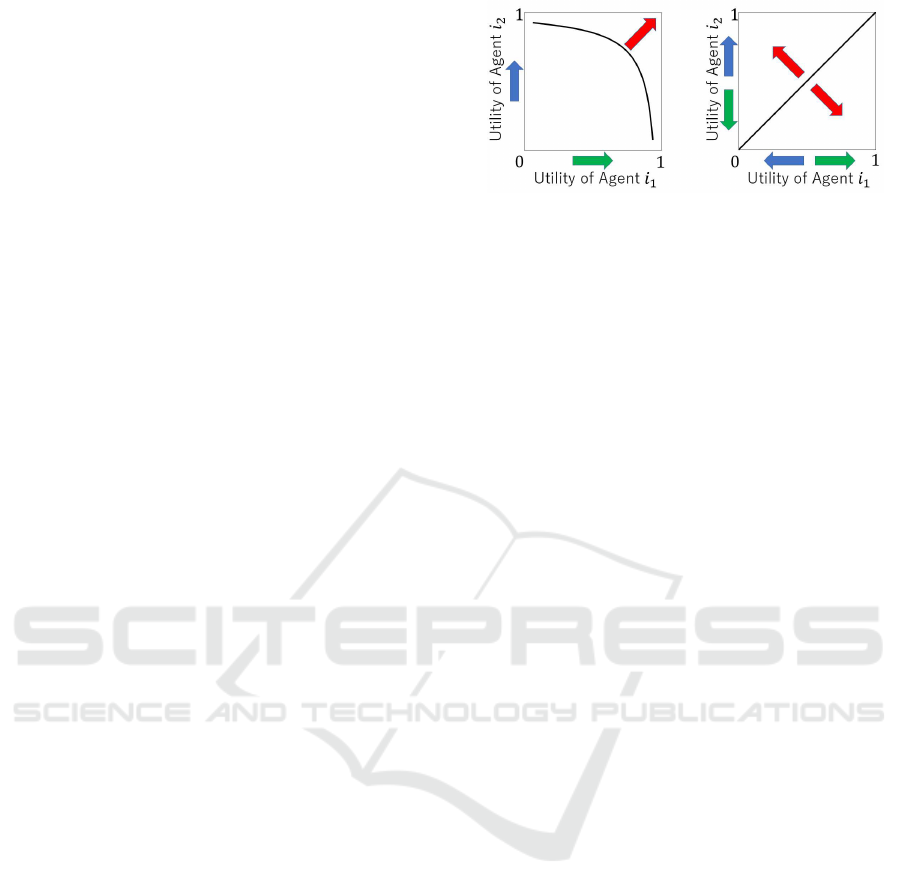
Figure 1: Utility spaces of non-competitive (left) and com-

petitive (right) bilateral negotiation.

3 COMPETITIVE BILATERAL

NEGOTIATION MODEL

In this section, we deﬁne competitive bilateral multi-

issue negotiation model. In addition, we show that

this negotiation with perfect information always leads

to an agreement in which the utility for both agents

are zero.

3.1 Basic Concept

As explained earlier, the objective of a rational agent

in conventional bilateral negotiations is to reach an

agreement that maximizes its own utility regardless

of that of the opponent. Conversely, the objective of

the agent in the competitive bilateral negotiation pro-

posed in this study is to maximize the difference in

utility between itself and the opponent. In this sense,

this negotiation can be regarded as a zero-sum game.

Therefore, even if high utility is obtained as a result

of negotiation, it is undesirable to bring high utility

to the opponent as well. Rather, it is desirable that the

difference in utility relative to the other party is larger,

even if one’s own utility is lower.

Figure 1 illustrates the difference between non-

competitive (left) and competitive (right) negotia-

tions. Here, the utility spaces of agents i

and i

each negotiation are shown, and the green and blue

arrows represent the vector of utility aimed at by i

and i

, respectively. In non-competitive negotiations,

the combined vector of both agents is indicated by a

red arrow. This means that the goal of the agents is to

reach agreement on the Pareto frontier represented by

the curved line. On the contrary, in competitive ne-

gotiations, each agent aims both to maximize its own

utility and minimize that of the opponent. Therefore,

the combined vectors of each agent are opposite to

each other as indicated by the red arrows. This im-

plies that each agent aims to reach an agreement on

its own side of the diagonal line that indicates a rela-

tive utility of zero for both agents.

Strategy Analysis for Competitive Bilateral Multi-Issue Negotiation

405

3.2 Formal Model

The formal model of negotiation is deﬁned as a tu-

ple of the following components: a set of negotiation

agents, negotiation domain (often called the outcome

space), negotiation protocol, and preference proﬁles.

(The paper (Baarslag et al., 2016) presents a survey

that provides more details.)

Let I be the set of negotiation agents. Because

this study deals only with bilateral negotiations, we

ﬁx I = {i

}. We also use the notation −i to indicate

the opponent of agent i ∈ I. The negotiation domain,

or often called the outcome space (denoted by O) rep-

resents the set of all possible negotiation outcomes.

The negotiation protocol determines the rules of ne-

gotiation, such as the order of offers and the condi-

tions of agreement. The preference proﬁle is a binary

relation over the negotiation domain for each agent,

that determines which of any two outcomes is more

preferable. Here, we follow the game-theoretic con-

vention and deﬁne the relation by a utility function

: O → R (for i ∈ I). However, in competitive nego-

tiations, the goal is to maximize the difference in util-

ities between the two agents. Therefore, in addition to

the usual utility function, we introduce RU

: O → R,

which represents the relative utility. The formal deﬁ-

nitions of these components are given below.

3.2.1 Negotiation Domain

The negotiation domain O is represented as a product

of one or more sets (called issues) of possible out-

comes. The set of indices for the issues is represented

by J = {1,..., j}, where j is the number of issues.

The set of outcomes for each issue is represented by

(k ∈ J), and thus O is deﬁned to be O

× ·· · × O

3.2.2 Negotiation Protocol

As with many previous studies on bilateral negotia-

tions, we follow the alternating-offers protocol (Ru-

binstein, 1982), in which agents take turns making

suggestions while searching for a mutually acceptable

outcome. More speciﬁcally, an agent with turn pro-

poses one of the elements of the negotiation domain

as the content of offer. The other agent who received

the proposal selects one of the following three actions.

Accept: Agree to the proposal. Both agents obtain

utility based on the agreed outcome.

Offer (Counter-offer): Reject the proposal and

make a new offer to the other party.

EndNegotiation: Reject the proposal and end the ne-

gotiation. Both agents receive a utility of zero.

Times (steps) in the progress of negotiation are rep-

resented by discrete values t = 1,2,... ∈ T . Negotia-

tions may have a time limit (denoted by t

max

) and, if

no agreement is reached within it, both agents gain a

utility value of zero.

3.2.3 Preference Proﬁle

The utility of agent i ∈ I for outcome o ∈ O is deﬁned

by the following equation:

(o) = Σ

k=1

where w

denotes the weight assigned to agent i for

issue k, satisfying Σ

k=1

= 1. V

: O

→ R is the

evaluation function for issue k for agent i. Accord-

ing to convention, in this study, the range of utility is

deﬁned as [0,1] ⊆ R.

3.2.4 Relative Utility Function

A relative utility function RU

: O → R is introduced

to represent the difference between the utility of the

two parties in a competitive negotiation. This is de-

ﬁned as

(o) = U

(o) −U

−i

(o).

3.3 Analysis of Perfect Information

Case

In competitive negotiations, if the agents’ preference

proﬁles are common knowledge, the utility for both

agents will be always zero. We demonstrate this fact

in game theory.

Here, we assume that the negotiation has a time

limit t

max

and that the utility function of the agents is

common knowledge. First, let i be the agent having

a turn at time t

max

and consider the optimal action of

i at this time. At t

max

, i can choose only Accept or

EndNegotiation, and if offer o made by −i at t

max

−

1 satisﬁes RU

(o) > RU

−i

(o), i can obtain a positive

relative utility by choosing Accept. Otherwise (i.e.,

(o) ≤ RU

−i

(o)), and i obtains relative utility zero

by choosing EndNegotiation. Thus, at t

max

− 1, −i

should offer o

with U

) ≤ U

−i

), which results

in a ﬁnal relative utility of zero for both agents. Using

the same argument in the reverse direction, we ﬁnd

that at any time t < t

max

, both agents make offers with

positive relative utility, leading to the same result.

4 NEGOTIATION STRATEGIES

This section presents some possible strategies for

competitive negotiations, the effectiveness of which

is analyzed empirically in the next section.

ICAART 2023 - 15th International Conference on Agents and Artiﬁcial Intelligence

406

4.1 Tactics

In general, negotiation comprises two decisions:

choosing an outcome from the negotiation domain as

one’s own offer and deciding whether to accept the

opponent’s offer. To decide what to offer, a plausible

approach is to set a target value (i.e., the minimum

acceptable relative utility) in advance, and make an

offer that exceeds this target. Furthermore, there are

two possible ways to select an outcome to offer: one

is to select an outcome randomly that exceeds the tar-

get value, and the other is to select an outcome that the

opponent is more likely to accept. To decide whether

to accept an offer, a plausible approach is to set a tar-

get value in advance, and agree to the opponent’s offer

if it exceeds the target value. Here, these two target

values may generally differ and may vary with time.

Below, we discuss possible tactics for each of

these decisions.

4.1.1 Tactics to Decide Target Value for Offer

Algorithm 1: Evaluation of T RU with prediction-dependent

tactic.

1: Update U

−i

est(i)

and U

est(i)

2: for all o ∈ O do

3: if RU

(o) = T RU

then

4: if U

−i

est(i)

(o) − U

est(i)

(o) > U

−i

est(i)

t−2

) −

est(i)

t−2

) then

5: O

.add(o)

6: end if

7: end if

8: end for

9: if O

6= ø then

10: T RU

= T RU

11: else

12: T RU

= T RU

− c

13: end if

There are two main approaches to determine the target

relative utility for an agent’s offer. The ﬁrst ﬁxes the

value through negotiation (called ﬁxed-value tactic)

and the second allows it to vary over time. The lat-

ter can be classiﬁed further into two types: the time-

dependent tactic, in which the target value is deter-

mined depending only on time, and the prediction-

dependent tactic, in which the target value is deter-

mined depending both on time and on predictions

about preferences.

The deﬁnitions of these three tactics are given be-

low, where T RU

is used to denote the target value of

agent i.

Fixed-Value Tactic: This tactic always sets the target

value to any value greater than zero.

Time-Dependent Tactic: The target value of agent i

in this tactic is deﬁned as follows:

T RU

= min

+ (1 − α

(t)) × (max

− min

This tactic is based on the idea of (Faratin et al.,

1998). Here, min

(called the reservation value) and

max

denote the minimum and maximum relative util-

ities that agent i desires in negotiation regardless of

time, respectively.

The function α

: T → R is called a time-

dependent function, and satisﬁes both α

(0) = κ

and

max

) = 1 (where κ

is a constant). Various time-

dependent tactics can be deﬁned according to the def-

inition of this function. Some well-known ways of

deﬁning this function include polynomials and expo-

nential functions. In this study, the following polyno-

mial function is used:

(t) = κ

+ (1 − κ

) × (min(t,t

max

)/t

max

)

1/β

This function changes the speed of concession de-

pending on the value of β. When β = 1, yielding pro-

gresses at a constant rate (linear); when β > 1, yield-

ing progresses early; and when β < 1, few conces-

sions are made while time t is small, whereas conces-

sions are suddenly made near t

max

Prediction-Dependent Tactic: This is introduced in

this study for competitive negotiation. This tactic

makes the following types of predictions:

• Prediction of the opponent’s preference.

• Prediction about how the opponent will predict

one’s own preference.

Based on these predictions, the target value is set tak-

ing into consideration whether the offer will be ac-

cepted by the opponent and the current time.

The detailed algorithm to determine the target

value is as follows. Let U

−i

est(i)

be the preference func-

tion of −i predicted by agent i, and let U

est(i)

be the

prediction of U

est(−i)

by agent i.

The algorithm for the target value T RU

at time

t for agent i is described in Algorithm 1. Here, o

t−2

denotes the previous offer by agent i, O

denotes the

set of candidates of offers(i.e., the set of possible of-

fers expected to yield a relative utility that matches

the target value TRU for agent i at time t), and c de-

notes the amount of change in the target value when

agent i concedes.

As shown in Algorithm 1 below, this tactic does

not change the target value if there is an offer that

the opponent is more likely to agree with that has the

same target value as the previous offer. Otherwise, the

target value is decreased.

Strategy Analysis for Competitive Bilateral Multi-Issue Negotiation

407

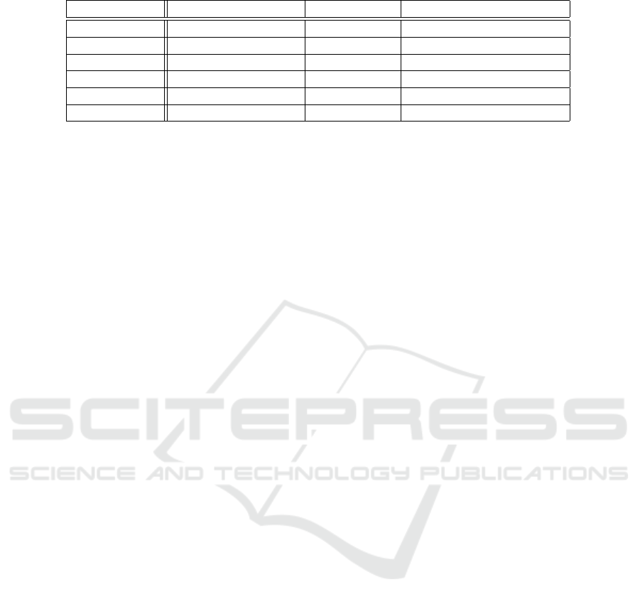
Table 1: Strategies for competitive bilateral negotiation.

Strategy name Target value for offer Offer choice Target value for agreement

PMT Prediction-dependent Mislead Time-dependent

TRT Time-dependent Random offer Time-dependent

PMF Prediction-dependent Mislead Fixed

TRF Time-dependent Random offer Fixed

FMF Fixed Mislead Fixed

FRF Fixed Random offer Fixed

4.1.2 Tactics for Offer Choice

There are two main approaches to choose an offer.

The ﬁrst, called the random offer tactic, chooses an

offer randomly from the set of offers that might bring

a relative utility above the target value. The second

approach, called mislead tactics, is proposed in this

study for competitive negotiation. This uses the pre-

diction of the opponent’s preference as well as the

prediction of how the opponent will predict one’s own

preference. Based on these predictions, the offer to be

selected is the one that the opponent is most likely to

accept from among the possible outcomes exceeding

the current target value. The formal deﬁnition of this

tactic is as follows: Let O

be the set of candidates for

the target value of agent i at time t. Offer o

at time t

by mislead tactics is then expressed as follows:

= argmax

o∈O

−i

est(i)

(o) −U

est(i)

(o)).

4.1.3 Tactics for Determining Agreement

Tactics on agreement can be divided into two cate-

gories, depending on whether the target value is ﬁxed

or variable. In both cases, agreement is chosen when

the predetermined target value is exceeded. Similar to

the target value used to determine the offer, tactics can

be time-dependent or prediction-dependent. Only the

simple time-dependent tactic is analyzed in this study.

4.2 Negotiation Strategies

Negotiation strategies are realized by combining the

tactics described above. Therefore there are 12 strate-

gies, consisting of three tactics to determine the target

value for the offer, two to choose the content of the

offer, and two to determine the target value as the cri-

terion for agreement. Of particular interest are the six

strategies shown in Table 1.

5 EXPERIMENTS

In order to evaluate the usefulness of the proposed

negotiation strategy, we conducted experiments in

which the strategies deﬁned in Section 4 were negoti-

ated with each other.

5.1 Parameter Settings

5.1.1 Negotiation Domain

The negotiation domain used in the experiments con-

sisted of three issues, each with ten options. The ne-

gotiation domain therefore consisted of a set of 1,000

outcomes.

5.1.2 Negotiation Strategies

For the experiments, we developed negotiation agents

for each of the six strategies deﬁned in the previous

section, whose parameter settings were presented be-

low.

For the time-dependent tactic, the values of the

four parameters are as follows.

• min = 0.05.

• max = 1.0.

• κ = 0.1.

• β = 1.0.

For the prediction-dependent tactic, the parameter

c for concession is set to 0.05. However, if this tactic

makes a concession resulting in T RU ≤ 0, to prevent

the agent from making an offer that would hurt itself,

the value of T RU was updated to 0.05 and chose an

offer satisfying RU > 0. In the experiment, the offers

based on the random-offer tactic and mislead tactic

were selected within the range of 0.02 round the value

of T RU . This is because the agent may not ﬁnd an

offer that yields utility exactly equal to T RU . Thus,

the agent set the value of T RU at time t to RU (o

t−2

)

(where o

t−2

denotes the previous offer), and decided

whether to make concession by Algorithm 1.

5.1.3 Preferences

The preferences deﬁned by the weights and utility

functions for i

and i

were set as follows, respec-

tively. Here, the same utility functions were used for

all issues.

ICAART 2023 - 15th International Conference on Agents and Artiﬁcial Intelligence

408

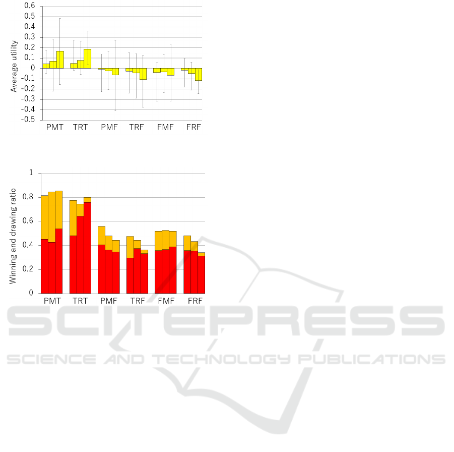
Figure 2: Average utility for each strategy when the cosine

similarities of predictions were 0.99, 0.95, and 0.9.

Figure 3: Win rate (denoted by red) and draw rate (denoted

by orange) for each strategy when the cosine similarities of

predictions were 0.99, 0.95, and 0.9.

• w

= (0.2,0.3,0.5).

• V

= (0.1,0.2,0.3,0.4,0.5,0.6,0.7,0.8,0.9,1.0).

• w

= (0.5,0.3,0.2).

• V

= (1.0,0.9,0.8,0.7,0.6,0.5,0.4,0.3,0.2,0.1).

Each agent i was not informed about the exact

preferences of its opponent. Instead, it was initially

informed of its own and its opponent’s preferences

with a certain range of error, which mimicked the pre-

dicted value U

−i

est(i)

and U

est(i)

. Speciﬁcally, for each

of the weights of the agents’ preferences and the eval-

uation functions, we gave predictions with errors such

that the cosine similarity is 0.99,0.95 and 0.9. Here,

since the difference between the preferences of it’s

own and the opponent can be large or small depend-

ing on the predicted values, in the experiment all of

the cases were evaluated.

5.2 Experimental Results

Under the settings described in the previous section,

the results of round-robin matches with six negotia-

tion strategies are shown below.

Figure 2 shows the average utility obtained by

each strategy. Here, the horizontal axis represents

the results of each strategy, and the three graphs show

the results when the cosine similarities of the prefer-

ence predictions are 0.99, 0.95, and 0.90, respectively,

from the left. The vertical axis shows average utilities

with their maximum and minimum values.

Figure 3 shows the sum of the win and draw rates

for each strategy. Here, the horizontal axis represents

the results of each strategy, and the three graphs show

the results when the preference predictions have co-

sine similarities of 0.99, 0.95, and 0.90, respectively,

from the left. The vertical red and orange graphs rep-

resent win and draw rates, respectively.

As shown in Figure 2, PMT and TRT strategies

were found to be superior to the other strategies, with

a positive average utility regardless of the error rate

of prediction. Speciﬁcally, when the cosine similar-

ity of the preference predictions was 0.99, the aver-

age utilities of PMT and TRT strategies were about

0.043 and 0.049, respectively. Also, when the cosine

similarity was 0.9, the average utilities of these two

strategies were about 0.168 and 0.187, respectively.

On the other hand, the average utilities of the other

four strategies always had negative average utility.

From the above results, it can be seen that the

utility of both PMT and TRT strategies increases as

the difference in expectations increases. A possible

reason for this is that both the PMT and TRT strate-

gies have time-dependent target values for agreement.

The larger the prediction error, the greater the proba-

bility of making a wrong decision about one’s rela-

tive gain for a proposal, and the greater the probabil-

ity of a larger error in the value of that relative gain.

While other strategies choose to agree when their rel-

ative gains are large (relative utilities greater than 0),

the PMT and TRT strategies have stricter criteria for

agreement, so they are less likely to agree to an agree-

ment that will actually be to their detriment. As a re-

sult, the larger the forecast error, the higher the rela-

tive utility of the PMT and TRT strategies, suggesting

that having a time-dependent agreement target value

is important for competitive negotiation.

Figure 3 shows that PMT strategy had a lower win

rate than TRT strategy, but the sum of the draw rate

and the win rate was always the highest for the PMT

strategy. For example, when the cosine similarity of

preference predictions was 0.99, the win rates of PMT

and TRT strategies were about 0.452 and 0.482, re-

spectively. The draw rates for these strategies were

about 0.365 and 0.293 respectively. Thus, the sum

of the win and draw rates for PMT and TRT were

about 0.816 and 0.775, respectively, with 4.2 percent-

age point higher win or draw rate for the PMT strat-

egy.

Examples of the negotiation process for PMT and

Strategy Analysis for Competitive Bilateral Multi-Issue Negotiation

409

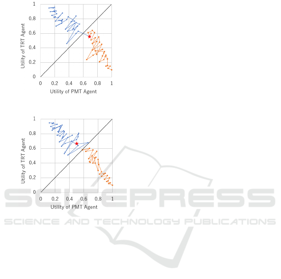
Figure 4: The negotiation process in which PMT won over

TRT by the largest utility margin.

Figure 5: The negotiation process in which PMT lost to

TRT by the largest utility margin.

TRT strategies are shown in Figures 4 and 5. Here,

the orange and blue plots indicate the history of the

offers by PMT and TRT agents, respectively, and the

red star indicates the agreed outcome. Figures 4 and

5 both show the results when the Cosine similarity of

the preference prediction was 0.99.

Figure 4 shows the negotiation process when PMT

wins TRT by the largest margin of utility. In Figure

4, neither agent agreed with the other’s offer and con-

tinued to make offers that were proﬁtable for them,

but in the end, TRT made a mistake and made an of-

fer that was more proﬁtable for PMT. As a result, the

utility of PMT became positive.

Figure 5 shows the negotiation process when PMT

lost by the largest margin of utility to TRT. In Figure

5, both agents made offers that were advantageous to

them until the end. However, in the end, PMT mispre-

dicted the utility of the offer received from TRT and

chose to agree, resulting in a negative utility for PMT.

In competitive negotiations, winning is important,

but not losing is also important. PMT strategy is also

an excellent strategy in terms of stability. Based on

the above results, the PMT strategy is considered to

be the optimal negotiation strategy in competitive ne-

gotiations.

6 CONCLUSIONS AND FUTURE

WORK

In this study, we proposed a model of competitive

bilateral multi-issue negotiation, in which an agent’s

utility and that of the opponent are evaluated relative

to each other and the actual utility can be regarded

as a zero-sum game. We also proposed a strategy for

the negotiations of this type, in which the basic idea

is to choose the offer that the opponent is most likely

to accept, based on the prediction of the opponent’s

preference and the prediction of one’s own preference

from the opponent’s perspective.

To demonstrate the effectiveness of the proposed

strategy, we conducted experiments in which agents

with various strategies negotiate competitive three-

issue bilateral negotiations. The results show that

the proposed strategy achieves the highest utility and

winning rate, regardless of the prediction error rate.

We also showed that time-dependent target value for

agreement is important for gaining relative utility in

competitive negotiations.

In future work, we will develop a prediction

method required in our negotiation setting, based on

some existing methods such as those using Bayesian

estimation (Lin et al., 2006) or heuristics (Jonker and

Robu, 2004). We are also interested in applying our

strategy to the development of agents that play board

games involving competitive negotiation.

REFERENCES

An, B., Lesser, V., and Sim, K. M. (2011). Strategic agents

for multi-resource negotiation. Autonomous Agents

and Multi-Agent Systems, 23(1):114–153.

Aydo

gan, R., Hindriks, K. V., and Jonker, C. M. (2014).

Multilateral mediated negotiation protocols with feed-

back. In Novel insights in agent-based complex auto-

mated negotiation, pages 43–59. Springer.

Baarslag, T., Hendrikx, M. J., Hindriks, K. V., and Jonker,

C. M. (2016). Learning about the opponent in au-

tomated bilateral negotiation: a comprehensive sur-

vey of opponent modeling techniques. Autonomous

Agents and Multi-Agent Systems, 30(5):849–898.

Cao, M., Luo, X., Luo, X. R., and Dai, X. (2015). Auto-

mated negotiation for e-commerce decision making: a

goal deliberated agent architecture for multi-strategy

selection. Decision Support Systems, 73:1–14.

ICAART 2023 - 15th International Conference on Agents and Artiﬁcial Intelligence

410

CATAN GmbH (n.d.). Welcome to the World of CATAN.

Retrieved January 6, 2023 from https://www.catan.

com/.

Faratin, P., Sierra, C., and Jennings, N. R. (1998). Ne-

gotiation decision functions for autonomous agents.

Robotics and Autonomous Systems, 24(3-4):159–182.

Fatima, S. S., Wooldridge, M. J., and Jennings, N. R.

(2006). Multi-issue negotiation with deadlines. Jour-

nal of Artiﬁcial Intelligence Research, 27:381–417.

Jennings, N. R., Faratin, P., Lomuscio, A. R., Parsons, S.,

Sierra, C., and Wooldridge, M. (2001). Automated

negotiation: prospects, methods and challenges. Inter-

national Journal of Group Decision and Negotiation,

10(2):199–215.

Jonker, C. and Robu, V. (2004). Automated multi-attribute

negotiation with efﬁcient use of incomplete preference

information. Available at SSRN 744047.

Keizer, S., Guhe, M., Cuay

ahuitl, H., Efstathiou, I., En-

gelbrecht, K.-P., Dobre, M., Lascarides, A., Lemon,

O., et al. (2017). Evaluating persuasion strategies and

deep reinforcement learning methods for negotiation

dialogue agents. ACL.

Kiruthika, U., Somasundaram, T. S., and Raja, S. (2020).

Lifecycle model of a negotiation agent: A survey of

automated negotiation techniques. Group Decision

and Negotiation, 29(6):1239–1262.

Lin, R., Kraus, S., Wilkenfeld, J., and Barry, J. (2006).

An automated agent for bilateral negotiation with

bounded rational agents with incomplete information.

Frontiers in Artiﬁcial Intelligence and Applications,

pages 270–274.

Mansour, K. and Kowalczyk, R. (2015). An approach to

one-to-many concurrent negotiation. Group Decision

and Negotiation, 24(1):45–66.

Rubinstein, A. (1982). Perfect equilibrium in a bargaining

model. Econometrica: Journal of the Econometric

Society, 50(1):97–109.

Zheng, X., Martin, P., Brohman, K., and Da Xu, L. (2014).

Cloud service negotiation in internet of things envi-

ronment: A mixed approach. IEEE Transactions on

Industrial Informatics, 10(2):1506–1515.

Strategy Analysis for Competitive Bilateral Multi-Issue Negotiation

411