A Rank Aggregation Algorithm for Performance Evaluation in Modern

Sports Medicine with NMR-based Metabolomics

∗

V. Vigneron

and H. Maaref

Univ. Evry, Université Paris-Saclay, IBISC EA 4526, Evry, France

Keywords:

Deep Learning, Pooling Function, Rank Aggregation, LBP, Segmentation, Contour Extraction.

Abstract:

In most research studies, much of the gathered information is qualitative in nature. This article focuses on

items for which there are multiple rankings that should be optimally combined. More speciﬁcally, it describes

a supervised stochastic approach, driven by a Boltzmann machine capable of ranking elements related to

each other by order of importance. Unlike classic statistical ranking techniques, the algorithm does not need

a voting rule for decision-making. The experimental results indicate that the proposed model outperforms

two reference rank aggregation algorithms, ELECTRE IV and VIKOR, and it behaves more stable when

encountering noisy data.

1 INTRODUCTION AND

RELATED WORKS

In the last decades, the ﬁeld of multiple criteria

decision-making (MCDM) has received considerable

attention in engineering, sciences, and humanities as

they are extremely efﬁcient in situations where pol-

icymakers need to decide priorities (Yazdani et al.,

2017).

There are optimal resolution procedures like lin-

ear programming or nonlinear optimization for solv-

ing problems governed by single criteria. But real-life

situations demand the evaluation of a set of alterna-

tives against multiple criteria and are typically struc-

tured as MCDM problems (Thakkar, 2021; Rahman

et al., 2017). When a decision needs to be made - like

choosing a movie, buying a car, selecting a stock port-

folio, etc. - the choice should not be random or biased

by someone’s suggestion. MCDM algorithms often

produce conﬂicting results when compared together

because of the choice of the function to optimize.

This comes from the unavoidable trade-off be-

https://orcid.org/0000-0001-5917-6041

https://orcid.org/ 0000-0002-1192-7333

∗

This research was supported by the program Cátedras

Franco-Brasileiras no Estado de São Paulo, an initiative of

the French consulate and the state of São Paulo (Brazil).

We thank our colleagues Rémi Souriau for his helpful com-

ments and Laurence Le-Moyec who supervise the data ac-

quisition with the Institut national du sport, de l’expertise et

de la performance (INSEP).

tween conﬂicting objectives as well as constraints. As

a result, the optimal solution is not unique and cor-

responds to a so-called Pareto solution (Freund and

Williamson, 2015).

On the opposite, learning to rank (LTR) is a class

of approaches that apply supervised machine learn-

ing (ML) to resolve ranking problems. The training

data for a LTR model consists of a list of samples and

a "ground truth" score for each of those samples, man-

ually labeled by experts, see (Li et al., 2017). The

set of ranked data ("ground truth") becomes the data

set that the system "trains" by minimizing some loss

function to learn how best to rank automatically these

items (Chaudhuri and Tewari, 2015).

The most common application of LTR is search

engine ranking (Sharma et al., 2022). We propose to

use them in the context of sports medicine because

performance evaluation is a kind of fuzzy task.

Existing LTR algorithms may be divided into

3 main classes: (a) pointwise methods which re-

duce the rating on each item to regression or clas-

siﬁcation (Blackburn and Ukhov, 2013) (b) pairwise

methods which essentially formulate ranking on each

document pair as a classiﬁcation problem (Burges

et al., 2007) (c) list-wise methods which optimize a

measure-speciﬁc loss function, on all available items.

See Chavhan et al.(Chavhan et al., 2021) for a review.

The pros and cons of using LTR vs. MCDM

are (a) LTR is essentially a black box in terms of

explainability. It’s hard to explain what exact ef-

fect speciﬁc inputs have on the outcome (b) LTR is

332

Vigneron, V. and Maaref, H.

A Rank Aggregation Algorithm for Performance Evaluation in Modern Sports Medicine with NMR-based Metabolomics.

DOI: 10.5220/0011798000003414

In Proceedings of the 16th International Joint Conference on Biomedical Engineering Systems and Technologies (BIOSTEC 2023) - Volume 4: BIOSIGNALS, pages 332-339

ISBN: 978-989-758-631-6; ISSN: 2184-4305

 2023 by SCITEPRESS – Science and Technology Publications, Lda. Under CC license (CC BY-NC-ND 4.0)

greedy (c) result relevance is metric-dependent. This

work presents a new extension of the LTR based on

a continuous restricted Boltzmann machine (CRBM)

(Hinton, 2002). The CRBM is a generative stochastic

artiﬁcial neural networks (ANN) that can learn a prob-

ability distribution over (all possible permutations of)

its set of inputs. CRBMs have found applications in

dimensionality reduction (Vrábel et al., 2020), clas-

siﬁcation (Yin et al., 2018) and collaborative ﬁltering

(Verma et al., 2019). They are excellent generative

learning models for latent space extraction. Specif-

ically, they can be trained into excellent ranking de-

vices because of their ﬂexible loss function and the

associative memory captured in the transfer matrix W

between the visible and the hidden layers, which is a

promising advantage over other standard MCDM al-

gorithms.

The paper is organized as follows: section 2 pro-

vides a detailed description of the problem and the

metrics used for measuring aggregation of ranks. Sec-

tion 3 presents the generative model. The experimen-

tal results are presented in Section 4. The last section

concludes and outlines the way for future work.

Notations. Throughout this paper small Latin let-

ters a, b,.. . represent integers. Small bold letters a, b

are put for vectors, and capital letters A, B for ma-

trices or tensors depending on the context. The dot

product between two vectors is denoted < a, b >. We

denote by ∥a∥ =

√

< a, a >, the ℓ

norm of a vector.

,. . ., X

are non ordered variates, x

,. . ., x

non or-

dered observations. "Ordered statistics" means either

(1)

≤. . . ≤ p

(n)

(ordered variates) or p

(1)

≤. . . ≤ p

(n)

(ordered observations). The p

(i)

are necessarily de-

pendent because of the inequality relations among

them.

Deﬁnition 1 ((Savage, 1956)). The rank order cor-

responding to the n distinct numbers x

,. . ., x

is the

vector t = (t

,. . .,t

)

where t

is the number of x

’s≤

and i ̸= j.

The rank order t is always unambiguously deﬁned

as a permutation of the ﬁrst n integers.

2 GENERAL FRAMEWORK

2.1 Rank-Aggregation

Let A = {a

,. . ., a

} be a set of alternatives, candi-

dates, individuals, etc. with cardinality |A|= n and let

V be a set of voters, judges, criteria, etc. with |V |= m.

The data is collected in a (n ×m) table T of general

term {t

i j

} crossing the sets A and V (Figure 1). t

i j

can be marks (t

i j

∈ N), value scales (t

i j

∈ R), ranks

(such that a voter can give ex-aequo positions) or bi-

nary numbers (t

i j

∈ {0, 1} such as opinion yes/no).

T represents the ranking of the n alternatives under

the form (see (Brüggemann and Patil, 2011) for a re-

minder on rank-aggregation). For ease of writing, in

the following, t

i j

= t

( j)

T =

(1)

(2)

... v

(k)

... v

(m)

. . . t

i j

(a) Data matrix T (t

i j

≥ 0).

→

(k)

. . . a

. . . y

(k)

i j

(b) kth pairwise comparison matrix between the

alternatives a

and a

Figure 1: The data are collected in a (n ×m) table T .

Solving a rank-aggregation problem means ﬁnd-

ing a distribution of values x

∗

attributed by a virtual

judge to the n alternatives by minimizing the dis-

agreements of opinions between the m judges (Ben-

son, 2016), i.e.

∗

= arg min

∑

k=1

d(t,t

(k)

), s.t. t ≥ 0, (1)

where d(t,t

(k)

) is a metric measuring the proximity

between t and t

(k)

, chosen a priori, and t

(k)

is the kth

column of the table T . Depending on the properties of

d(·), we will deal with a nonlinear optimization pro-

gram with an explicit or implicit solution.

One could also stand the dual problem of the

previous one, i.e., is there a distribution of rank-

ings/marks that the m voters could have attributed to

a virtual alternative ’a’ summarizing the behavior of

the set of individuals A (Yadav and Kumar, 2015)?

The ﬁrst problem is linked to the idea of aggregating

points of view, and the second to the concept of sum-

marizing behaviors.

A Rank Aggregation Algorithm for Performance Evaluation in Modern Sports Medicine with NMR-based Metabolomics

333

2.2 Explicit or Implicit Resolution

Eq. (1) deﬁnes a nonlinear optimization program

whose solution is x

∗

(Yadav and Kumar, 2015). The

distance d(t

(k)

′

)

) between the ranking of voters k

and k

′

can be chosen for instance as the Euclidean

distance

∑

i=1

−t

′

)

, the disagreement distance

(Condorcet)

∑

i=1

sgn|t

−t

′

| or the order disagree-

ment distance

∑

(k)

i j

−y

′

)

i j

|as t

(k)

can be replaced

by its permutation matrix Y

(k)

(Figure 1). In the lat-

ter, y

(k)

i j

i< j

denotes the indicator matrix for which

(k)

i j

= 1 if the rank of the alternative a

is less than the

alternative a

and 0 otherwise (Gehrlein and Lepelley,

2011). Note that y

(k)

= 0 and y

(k)

i j

= 0 if i and j are

ex-aequos.

In using matrix Y

(k)

∑

(k)

i j

− y

′

)

i j

| =

∑

(k)

− y

′

)

since since the expressions

(k)

i j

−y

′

)

i j

| are 0 or 1.

As y

i j

= y

i j

= y

(k)

i j

= y

(k)

i j

= 0 or 1, the function

associated to order disagreement distance d is given

∑

i=1

∑

j=1

i j

∑

i=1

∑

j=1

∑

k=1

i j

−2

∑

i=1

∑

j=1

i j

∑

k=1

(k)

i j

(2)

Let α

i j

∑

k=1

(k)

i j

the total number of voters prefer-

ring alternative a

to a

and deﬁne a matrix A = {α

i j

summing the m matrices Y

(k)

associated to the rank-

ings t

(k)

of the voters V

(k)

, Eq. (2) becomes:

∑

i=1

∑

j=1

i j

∑

i=1

∑

j=1

i j

−2

∑

i=1

∑

j=1

i j

. (3)

Finally, the search for a total order given by a matrix

Y is the solution of the linear program

max

∑

i=1

∑

j=1

i j

∑

i=1

∑

j=1

i j

−2

∑

i=1

∑

j=1

i j

s.t. α

i j

∑

k=1

(k)

i j

+ y

= 1, i < j,

= 0 y

i j

+ y

−y

≤ 1, i ̸= j ̸= k, y

i j

∈ {0, 1}.

(4)

If the chi-2 metric is chosen, then the dependent

variables cannot be separated as in Eq. (4): The reso-

lution follows an implicit gradient-descent procedure

as in (Vigneron and Tomazeli Duarte, 2018). Section

2.3 detailed how chi-2 distance is used for solving ag-

gregation problems.

2.3 Chi-2 Metric

The distance between x and t

(k)

is given by

d(x,t

(k)

) =

∑

i·



·x

−

·k



, (5)

where

i·

∑

+ x

∑

·x

∑

·k

∑

(6)

Let n¯r =

∑

,n ¯x =

∑

·k

∑

and t

i·

∑

Then, after some calculus, the optimal ranking x

∗

minimizes

∑

d(x,t

(k)

∑

k=1

∑

i=1

¯r + ¯x

i·

+ x



n ¯x

−

·k



= n(¯r + ¯x)

∑

i=1

∑

k=1



√

i·

n ¯x

−

√

i·

·k



(7)

assuming t

i·

≫ x

and

√

i·

+ x

≈

√

i·

According to Eq. (7), the ranking is performed

on the row proﬁles or column-proﬁles of the matrix T

(see Fig. 1), each row being weighted by

√

i·

So it is equivalent to compute proﬁle matrix C

whose entry is

√

i·

·k

, to consider the Euclidean dis-

tance between its rows and to heighten each row by

√

i·

. A remark has to be made at this stage: two al-

ternatives will be close if a large proportion of judges

choose them simultaneously. For example, if there is

a considerable amount of individuals chosen prefer-

ably by judges ’A’ and ’B,’ then we will say that

judges A and B are close and that they "attract" each

other. Eq. (7) is the well-known expression used in

testing for independence in contingency tables.

Eq. (7) derives from the Bhattacharyya directed

divergence between two discrete probability distri-

butions P = {p

} and Q = {q

} deﬁned as BD =

−ln(

∑

√

) (Nielsen, 2022) if p

i·

¯x

and q

i·

·k

. Note that n

is useless in the ratio and will be

removed in the entries of the continuous restricted

Boltzmann machine. Implicit methods are natural for

LTR algorithms that are usually fed by an incoming

data stream, n constantly varying. Section 3 proposes

a learning model in which the rank probabilities take

the form of a Boltzmann distribution.

BIOSIGNALS 2023 - 16th International Conference on Bio-inspired Systems and Signal Processing

334

3 METHODOLOGY

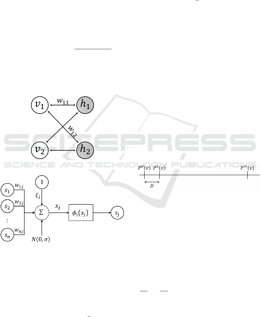
3.1 Continuous Restricted Boltzmann

Machine

Chen and Murray proposed another Boltzmann ma-

chine (BM) approach with continuous neuron in

(Chen and Murray, 2003): the CRBM, a restricted

Boltzmann machine using the neuron structure de-

picted in ﬁgure 2. In the CRBM, the activation func-

tion is unique for each neuron and given by:

= φ

) = θ

+ (θ

−θ

)

1 + exp(−a

)

(8)

where θ

and θ

are, respectively, the function’s

lower and upper bounds. a

is a slope parameter of

(.). The continuous behavior for the hidden units

allows us to capture more information than binary

units.

(a) Continuous restricted Boltzmann machine.

(b) Structure of the neuron j of a CRBM.

Figure 2: White neurons are visible neurons and gray neu-

rons are hidden neurons in the CRBM. the coefﬁcient w

i j

refers to the weight of the symmetric link between the i−th

visible unit v

and the j−th hidden unit h

We note W ∈ IR

(m×ℓ)

the transfer matrix between

the two layers and ξ

and ξ

the bias vectors of, re-

spectively, the visible layer and the hidden layer. The

energy function of the CRBM is:

E(v, h) = −v

W h −v

−h

∑

−1

′

)ds

′

(9)

with φ

−1

(.) the inverse of the activation for a coefﬁ-

cient slope a

= 1. The energy E(s) of a CRBM is

associated with the joint probability of the state of the

neurons P

cRBM

(s) deﬁned as

CRBM

(s) =

exp(−E(s)), (10)

where Z is a marginalization constant. Training a

CRBM is performed in minimizing the energy func-

tion Eq. (9), which itself requires sampling the hidden

units.

The CRBM training uses the contrastive diver-

gence algorithm (see (Hinton, 2012)). The training set

D = {v

}

1≤k≤n

is composed of n observations used to

ﬁnd the best set of parameters P = {W, ξ}, ξ regroup-

ing visible and hidden bias vectors.

Minimizing directly the joint log-likelihood

∑

k=1

logP

CRBM

) to update the parameters is difﬁ-

cult due to the presence of the constant Z. Then it

is replaced by the minimization of the contrastive di-

vergence (MCD) (Hinton, 2002) that minimizes the

contrast D between two successive Kullback-Leibler

(KL)-divergences:

D = KL(P

(v),P

∞

(v)) −KL(P

(v),P

∞

(v)), (11)

where P

(v),P

∞

(v),P

(v) are the distribution func-

tion of the visible units over respectively the training

set, the equilibrium state and after q steps of Gibbs

sampling (Hinton, 2012) (Fig. 3).

Figure 3: An intuitive idea is to minimize the KL divergence

between P

(v)P

∞

(v). But P∞(v) is intractable. We prefer

to minimize D. If D = 0, then P

(v) = P

(v) and then :

(v) = P

∞

(v).

An important observation is that any linear com-

bination of measures of discrepancy with positive co-

efﬁcients is also a measure of discrepancy.

KL(P

(v),P

∞

(v)) −KL(P

(v),P

∞

(v))

+λ(BD

(v) −BD

(v)),

(12)

with λ a regularization parameter. And thus, Eq. (12)

can be used as a measure of discrepancy.

In particular, the observations are normalized: v =

(

i·

·1

,. . .,

i·

·m

)

(see section 2.3).

In the next section, a CRBM driven by the loss

function (12) ranks rugby players according to their

performances measured by metabolomics.

A Rank Aggregation Algorithm for Performance Evaluation in Modern Sports Medicine with NMR-based Metabolomics

335

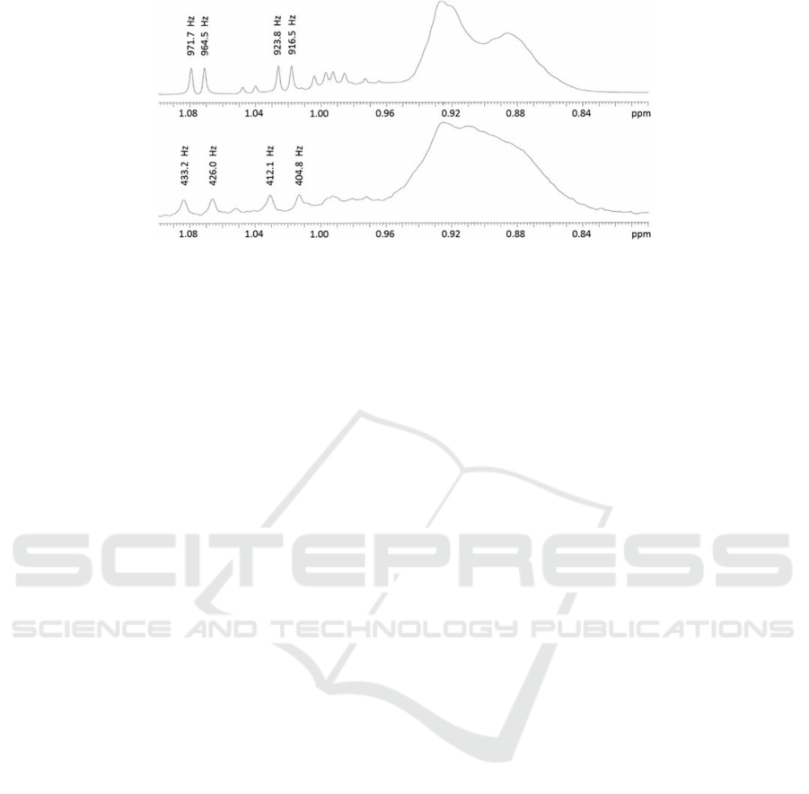
Figure 4:

H NMR spectrum of human plasma acquired at 900 (top) and 400 MHz (bottom), from (Louis et al., 2017).

4 EXPERIMENTS WITH

METABOLOMICS DATA

Endurance is a widely practiced sporting activity,

from novice to champion. It is deﬁned as maintaining

an effort for a prolonged period. This effort originates

from signiﬁcant physiological and metabolic stress

leading to organism adaptations. If this effort is too

great, it can cause metabolic and locomotor disorders.

The objective is to optimize training methods that will

protect the health of athletes, young or old, efﬁcient or

less efﬁcient. We adopt an integrative approach that

simultaneously studies the physiological responses to

exercise and the molecular and metabolic signals.

From multivariate statistical analysis of bioﬂuids such

as urine, serum, plasma, saliva, sweat, etc., it is pos-

sible to generate metabolomic proﬁles or biomark-

ers. See (Khoramipour et al., 2022) for a review of

metabolomics practice in sports medicine.

Since the 00’s metabolomics investigates quanti-

tatively the metabolome of living systems in response

to pathophysiological stimuli or genetic modiﬁcation

(Amara et al., 2022).

Nuclear magnetic resonance (NMR) is tradition-

ally used to elucidate molecular structures. It takes

advantage of the energy transition of nuclear spins in

a strong magnetic ﬁeld to identify and elucidate the

structure of organic molecules and speciﬁc metabo-

lites. Metabolites are intermediate organic com-

pounds resulting from metabolism. To understand the

metabolomic changes induced by endurance exercise

and training of rugby players according to the inten-

sity and duration of the activity, we study the physio-

logical modulation of rugby players according to their

positions.

The study focuses on the activity variability be-

tween the forwards - more intense and intermittent ef-

forts - and the rears - greater distance covered, more

running, more rest time, etc. (Paul et al., 2022). It

aims to answer whether, during matches, (a) the uri-

nary metabolites are identical before and after 80 min-

utes of a match? (b) this metabolomic modulation is

of the same order depending on the player’s position?

No study to date has investigated how to predict

physiological exertion in rugby or how to classify a

player according to its physiological parameters.

The experimental protocol is as follows: the urine

of 80 players (40 forwards and 40 rears) is analyzed

by NMR to identify the metabolites present in the

two situations described above. The variations in

metabolism explain the variations in physiological pa-

rameters as a function of the time and position factors.

NMR spectra contain more than 10,000 values. See

Fig 4 for an example of NMR spectrum.

19 variables represent the physiological vari-

ables, among which: forward/backward position

of the player during the match, body mass in-

dex, experience, playing time, distance covered on

the playground but also plasmatic metabolite rates

in phenylalanine, tyrosine, glucose, creatinine, β-

hydroxybutyrate, lactate, pyruvate, N-acetyl glyco-

protein, lipids (Table 1). This set of variables consti-

tutes the criteria that are used to rank the rugby play-

ers.

There are 70 samples in the training set and 10 in

the test set. The structure of the CRBM is: 19 visi-

ble and 3 hidden units. Due to the small training and

test data, we did not divide the data into mini-batches

during the experiment. All the data were divided

into eight groups for the seven-fold cross-validation

method. Seven groups were selected as the training

set each time, and the remaining group was the test

set. This process was repeated until each group be-

came a test set. The number of iterations was 200 for

each CRBM. For training, the CRBMs were initial-

ized with small random weights and zero bias param-

eters. The learning rate was η = 0.1 when training

with CD in Eq. (12) and λ = 0.005. CRBMs models

BIOSIGNALS 2023 - 16th International Conference on Bio-inspired Systems and Signal Processing

336

Table 1: Data description. Notice that variable 17 precises the position of the players. Forwards: pillars, hooker, 2nd lines.

Backward: 3rd lines, 9 and 10, backs.

Variables type (if real: µ± std.err.) physiological signiﬁcation

1 term binary 1st term=1, 2nd term=0

2 P binary position forward=1, backward=0

3 A 28,4 ±0.97 Age

4 H 179.95 ±1.0 height

5 W 89.75 ±2.81 weight

6 BMI 27.65 ±0.756 body-mass index

7 X 41,3 ±1.01 game experience

8 Ty 143,9 ±1.89 tyrosine

9 Glu 269,5 ±2.59 glucose

10 β 414, 1 ±3.22 β-hydroxybutyrate

11 Creat 6.57 ±0.22 creatinine

12 Gly 5069 ±11.25 glycoprotein

13 D 2.238 ±7.48 distance covered on the playground

14 L 51,6 ±1.13 lipids

16 R {1,2, 3} rolling position

17 PHC0 −86.98 ±15.73 phenylalanine 0

18 PHC1 23.36 ±9.19 phenylalanine 1

19 SNR 41.03 ±3.56 signal to noise ratio

Table 2: Test results comparing CRBM with classic MCDMs algorithms VIKOR and ELECTRE IV. Float numbers are issued

from the models and the ranks in sorting these numbers.

Players VIKOR ELECTRE IV CRBM+Bhattacharyya

1 3.608 7 3.127 1 3.291 1

2 5.123 1 6.324 6 6.074 7

3 4.639 6 5.094 8 4.925 8

4 5.378 8 4.923 7 5.088 6

5 5.811 3 6.147 4 5.886 3

6 4.033 2 3.401 3 3.693 4

7 3.468 4 3.567 10 3.467 5

8 4.254 10 3.411 5 3.663 10

9 5.6220 9 6.2400 9 5.9600 9

10 5.8110 5 6.3240 2 6.0740 2

are updated while the new training example is com-

pleted.

The results obtained with VIKOR, ELECTRE IV,

and the CRBM are gathered in Table 2 for compar-

ison. For each MCDM algorithm, the ﬁrst column

measures the discrepancy of the model Eq. (12) and

the second column the rank of the rugby player (in

bold). They provide an interpretation that the CRBM

method is closer to the actual results and far from

the ELECTRE IV method (Roy, 1985). VIKOR is

a MCDMs, ranking preferences among a set of al-

ternatives in the presence of conﬂicting criteria un-

der the concept of group regrets (Guiwu et al., 2020).

ELECTRE IV assumes that all requirements (actually

pseudo-criteria) have the same importance.

At ﬁrst glance, the rankings are not similar but not

so different either. The rankings order the players ac-

cording to the sportive qualities recorded in Tab. 1.

For example, ELECTRE IV and CRBM would select

player one ﬁrst, then player 10. But ELECTRE IV

would prefer player 6 in the third place while CRBM

would choose player 5.

The discriminant representation provided by the

hidden layer is the most determining factor in favor

of CRBM against VIKOR or ELECTRE. The players

were ranked by the ﬁrst hidden neuron of the CRBM.

The scatter-plot Figure 5 uses the values of the ﬁrst

two hidden neurons. This means the hidden neurons

capture a latent representation capable of discriminat-

ing between the two classes, "rears" and "forwards."

A Rank Aggregation Algorithm for Performance Evaluation in Modern Sports Medicine with NMR-based Metabolomics

337

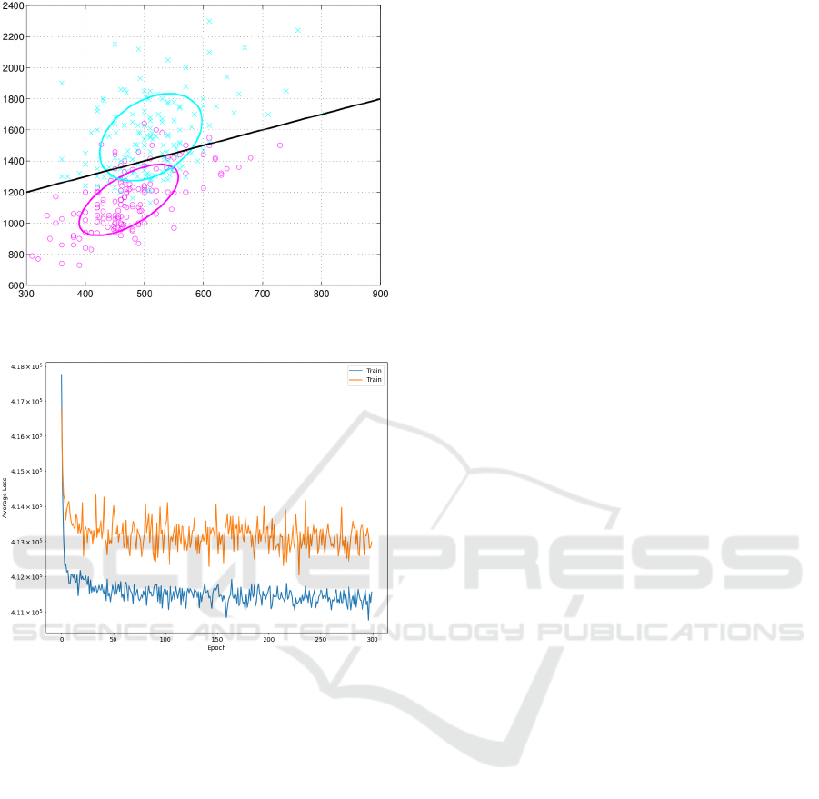
(a) Separated classes (before and after the match) obtained

from the values of the hidden neurons.

(b) Reconstruction error for the training (blues) and the test

(red) sets.

Figure 5: Score plot obtained with the two hidden neurons

of the restricted Boltzmann machine (RBM): the samples

separate each other before and after the match.

5 CONCLUSION AND

DISCUSSIONS

CRBMs are domain-independent feature extractor

that transforms raw data into latent variables. The

most relevant questions are: how to dimension the

hidden layer h optimally? And how do the neurons

interact?

Our generative network is relatively small. Hence

to compute p(h|v) is an affordable problem for small

RBM, but once we have a large number of hidden

neurons, it becomes impossible to compute all pos-

sible p(h|v). The more neurons, the more computa-

tional efforts are needed: massive networks should

not be the only way to reduce the modeling error. The

choice of dimension remains today an unsolved issue.

In addition, for each conﬁguration v, some hidden

neurons have a probability close to 0 or 1, meaning

that for each v, some states of h are irrelevant.

Besides being energy-consuming, a signiﬁcant di-

mension network requires much time to learn. In

many papers, authors focus on comparing the per-

formance between models but barely reach compu-

tational efforts between models. The issue of compu-

tational efforts can have a signiﬁcant impact, partic-

ularly in the real-time system. Still, it is enormously

dependent on the data, the application, and the used

hardware.

To reduce the bias between the data distribution

data

(x) and the estimated data distribution P

model

(x)

the cost function was modiﬁed (Eq. 12).

The next step is constructing a deeper network,

such as deep belief network (DBN), that may provide

more explainability hints.

REFERENCES

Amara, A., Frainay, C., Jourdan, F., Naake, T., Neumann,

S., Novoa-Del-Toro, E. M., Salek, R., Salzer, L.,

Scharfenberg, S., and Witting, M. (2022). Networks

and Graphs Discovery in Metabolomics Data Anal-

ysis and Interpretation. Frontiers in Molecular Bio-

sciences, 9.

Benson, D. (2016). Representations of Elementary Abelian

p-Groups and Vector Bundles. Cambridge tracts in

mathematics. Cambridge University Press, 1 edition.

Blackburn, D. and Ukhov, A. (2013). Individual vs. ag-

gregate preferences: The case of a small ﬁsh in a big

pond. Management Science, 59:470–484.

Brüggemann, R. and Patil, G. (2011). Ranking and Prior-

itization for Multi-indicator Systems: Introduction to

Partial Order Applications. Environmental and Eco-

logical Statistics. Springer-Verlag New York.

Burges, C., Ragno, R., and Le, Q. (2007). Learning to

rank with nonsmooth cost functions. In Schölkopf, B.,

Platt, J., and Hoffman, T., editors, Advances in Neu-

ral Information Processing Systems, volume 19. MIT

Press.

Chaudhuri, S. and Tewari, A. (2015). Perceptron like

algorithms for online learning to rank. ArXiv,

abs/1508.00842.

Chavhan, S., Raghuwanshi, M. M., and Dharmik, R. C.

(2021). Information retrieval using machine learning

for ranking: A review. Journal of Physics: Conference

Series, 1913(1):012150.

Chen, H. and Murray, A. (2003). Continuous restricted

boltzmann machine with an implementable training

algorithm. IEE Proceedings-Vision, Image and Sig-

nal Processing, 150(3):153–158.

Freund, D. and Williamson, D. (2015). Rank aggregation:

New bounds for MCx. CoRR, abs/1510.00738.

BIOSIGNALS 2023 - 16th International Conference on Bio-inspired Systems and Signal Processing

338

Gehrlein, W. and Lepelley, D. (2011). Voting Paradoxes and

Group Coherence: The Condorcet Efﬁciency of Voting

Rules. Studies in Choice and Welfare. Springer-Verlag

Berlin Heidelberg, 1 edition.

Guiwu, W., Jie, W., Jianping, L., Jiang, W., Cun, W., Fuad,

E., and Tasawar, H. (2020). Vikor method for multiple

criteria group decision making under 2-tuple linguis-

tic neutrosophic environment. Economic Research-

Ekonomska Istraživanja, 33(1):3185–3208.

Hinton, G. (2002). Training products of experts by mini-

mizing contrastive divergence. Neural computation,

14(8):1771–1800.

Hinton, G. (2012). A practical guide to training restricted

boltzmann machines. In Montavon, G., Orr, G. B.,

and Müller, K.-R., editors, Neural Networks: Tricks

of the Trade (2nd ed.), volume 7700, pages 599–619.

Springer.

Khoramipour, K., Sandbakk, O., Keshteli, A., Gaeini, A.,

Wishart, D., and Chamari, K. (2022). Metabolomics

in exercise and sports: A systematic review. Sports

Med., 52(3):547–583.

Li, X., Wang, X., and Xiao, G. (2017). A comparative study

of rank aggregation methods for partial and top ranked

lists in genomics applications. Brieﬁngs in Bioinfor-

matics, 20(1):178–189.

Louis, E., Cantrelle, F., Mesotten, L., Reekmans, G., and

Adriaensens, P. (2017). Metabolic phenotyping of hu-

man plasma by (1) h-nmr at high and medium mag-

netic ﬁeld strengths: a case study for lung cancer.

Magnetic resonance in chemistry : MRC, 55.

Nielsen, F. (2022). Statistical divergences between densi-

ties of truncated exponential families with nested sup-

ports: Duo bregman and duo jensen divergences. En-

tropy, 24(3).

Paul, L., Naughton, M., Jones, B., Davidow, D., Patel, A.,

Lambert, M., and Hendricks, S. (2022). Quantifying

collision frequency and intensity in rugby union and

rugby sevens: A systematic review. Sports Medicine -

Open, 8.

Rahman, A., Sungyoung, L., and Tae, C. (2017). Accurate

multi-criteria decision making methodology for rec-

ommending machine learning algorithm. Expert Sys-

tems with Applications, 71:257–278.

Roy, B. (1985). Methodologie multicritere d’aide a la deci-

sion. Economica, Paris,.

Savage, R. (1956). Contributions to the theory of rank-order

statistics – the trend case. The Annals of Mathematical

Statistics, 27(3):590–615.

Sharma, P., Yadav, D., Thakur, R. N., Reddy, K., and

Praveen, M. (2022). Web page ranking using web

mining techniques: A comprehensive survey. Mob.

Inf. Syst., 2022.

Thakkar, J. (2021). Multi-Criteria Decision Making.

Springer, ﬁrst edition.

Verma, S., Patel, P., and Majumdar, A. (2019). Col-

laborative Filtering with Label Consistent Re-

stricted Boltzmann Machine. arXiv e-prints, page

arXiv:1910.07724.

Vigneron, V. and Tomazeli Duarte, L. (2018). Rank-order

principal components. A separation algorithm for or-

dinal data exploration. In 2018 International Joint

Conference on Neural Networks, IJCNN 2018, Rio de

Janeiro, Brazil, July 8-13, 2018, pages 1–6.

Vrábel, J., Po

rízka, P., and Kaiser, J. (2020). Restricted

boltzmann machine method for dimensionality reduc-

tion of large spectroscopic data. Spectrochimica Acta

Part B: Atomic Spectroscopy, 167:105849.

Yadav, N.. author. abd Yadav, A. and Kumar, M. (2015). An

Introduction to Neural Network Methods for Differen-

tial Equations. Springer, Gurgaon, Haryana, India.

Yazdani, M., Fomba, S., and Zaraté, P. (2017). A Decision

Support System for Multiple Criteria Decision Mak-

ing Problems. In 17th International Conference on

Group Decision and Negotiation (GDN 217), pages

67–75, Stuttgart, Germany.

Yin, J., Lv, J., Sang, Y., and Guo, J. (2018). Classiﬁca-

tion model of restricted boltzmann machine based on

reconstruction error. Neural Computing and Applica-

tions, 29:1–16.

A Rank Aggregation Algorithm for Performance Evaluation in Modern Sports Medicine with NMR-based Metabolomics

339