On the Hardness and Necessity of Supervised Concept Drift Detection

∗

Fabian Hinder

, Valerie Vaquet

, Johannes Brinkrolf

, and Barbara Hammer

CITEC, Bielefeld University, Inspiration 1, Bielefeld, Germany

Keywords:

Concept Drift, Stream Learning, Drift Detection, No Free Lunch.

Abstract:

The notion of concept drift refers to the phenomenon that the distribution generating the observed data changes

over time. If drift is present, machine learning models can become inaccurate and need adjustment. Many

technologies for learning with drift rely on the interleaved test-train error to detect drift and trigger model

updates. This type of drift detection is also used for monitoring systems aiming to detect anomalies. In this

work, we analyze the relationship between concept drift and change of loss on a theoretical level. We focus

on the sensitivity, speciﬁcity, and localization of change points in drift detection, putting an emphasize on the

detection of real concept drift. With this focus, we compare the supervised and unsupervised setups which are

already studied in the literature. We show that, unlike the unsupervised case, there is no universal supervised

drift detector and that the assumed correlation between model loss and concept drift is invalid. We support our

theoretical ﬁndings with empirical evidence for a combination of different models and data sets. We ﬁnd that

many state-of-the-art supervised drift detection methods suffer from insufﬁcient sensitivity and speciﬁcity, and

that unsupervised drift detection methods are a promising addition to existing supervised approaches.

1 INTRODUCTION

The world that surrounds us is undergoing constant

change, which also affects the increasing amount of

data sources available. Those changes – referred to as

concept drift – frequently occur when data is collected

over time, e.g., in social media, sensor networks, IoT

devices, etc., and are induced by several causes such

as seasonal changes, changed demands of individual

costumers, aging, or failure of sensors, etc. Drift in

the data usually requires some actions being taken to

ensure that systems are running smoothly. These can

be either actions taken by a person or by the learning

algorithm (Ditzler et al., 2015).

Understanding the nature and underlying structure

of drift is important as it allows the user to make in-

formed decisions (Webb et al., 2017) and technical

systems to perform desirable corrections (Vaquet et al.,

2022). Depending on the context, different actions

have to be taken. There are two main problem se-

tups: Autonomously running systems need to robustly

https://orcid.org/0000-0002-1199-4085

https://orcid.org/0000-0001-7659-857X

https://orcid.org/0000-0002-0032-7623

https://orcid.org/0000-0002-0935-5591

∗

We gratefully acknowledge funding by the BMBF

TiM, grant number 05M20PBA.

solve a given task in the presence of drift. In this set-

ting, the learning algorithm of online learners needs

knowledge about the drift to update the model in a

reasonable way (Ditzler et al., 2015). In contrast, in

system monitoring, the drift itself is of interest as it

might indicate that certain actions have to be taken.

Examples of such settings are cyber-security, where

a drift indicates a potential attack, and the monitor-

ing of critical infrastructures such as electric grids or

water distribution networks, where drift indicates leak-

ages or other failures (Eliades and Polycarpou, 2010).

While system monitoring can minimize the damage

caused by a malfunctioning technical system, and re-

duce wastage of resources, applying adaptive online

learners can increase revenue in case of changing con-

sumer behaviors and is key to robot navigation and

autonomous driving (Losing et al., 2015).

Although both problem setups are very different,

the majority of approaches rely on (supervised) drift

detection, where the drift is detected by analyzing

changes in the loss of online models. This is an intu-

itive step in the setting of (supervised) online learning

as the goal is to minimize the interleaved test-train er-

ror by triggering model updates when drift is detected.

In the monitoring scenario, detecting drift by refer-

ring to a stream learning setup is a commonly used

surrogate for the actual problem.

164

Hinder, F., Vaquet, V., Brinkrolf, J. and Hammer, B.

On the Hardness and Necessity of Supervised Concept Drift Detection.

DOI: 10.5220/0011797500003411

In Proceedings of the 12th International Conference on Pattern Recognition Applications and Methods (ICPRAM 2023), pages 164-175

ISBN: 978-989-758-626-2; ISSN: 2184-4313

 2023 by SCITEPRESS – Science and Technology Publications, Lda. Under CC license (CC BY-NC-ND 4.0)

Considering stream learning in the presence of con-

cept drift, technologies commonly rely on windowing

techniques and adapt the model based on the charac-

teristics of the data in an observed time window. Such

methods rely on non-parametric methods and ensem-

ble technologies for (mostly supervised) online models.

Active methods explicitly detect drift, usually referring

to change of loss, and trigger model adaptation this

way, while passive methods continuously adjust the

model (Ditzler et al., 2015), hybrid approaches (Raab

et al., 2019) combine both approaches by continuously

adjusting the model unless drift is detected and a new

model is trained.

For many problems the precise pinpointing of the

timepoint of the drift event is mandatory to ensure an

optimal usage of the provided data: Only if we know

which samples were collected after the drift happened,

we can perform retraining or analysis in a consistent

way with respect to the current distribution. In ad-

dition to a precise pinpointing in time, a distinction

between virtual and real drift, i.e., non-stationarity of

the marginal distribution only or also the posterior,

can help to understand the dynamics of the drift and

inform consecutive steps.

The detection of drift, especially real drift is gener-

ally considered to be a hard problem (Hu et al., 2020).

Although many attempts were made to tackle the prob-

lem of constructing a general purpose detector for real

drift, it is still considered to be widely unsolved. Re-

cently theoretical results regarding the solubility were

published (Hinder et al., 2020, 2022) validating a large

class of common drift detection schemes from a the-

oretical perspective. However, those results focus on

drift detection in an unsupervised scenario only. To

the best of our knowledge, comparable results do not

exist for drift detection in a supervised setup, i.e., for

the detection of real drift.

The purpose of this contribution is to deepen the un-

derstanding of drift detection from a theoretical point

of view by analyzing the interconnection between con-

cept drift and learning algorithms. More precisely, we

consider the commonly assumed necessity of concept

drift detection for the validity of stream learning algo-

rithms (Gonçalves Jr et al., 2014; Gama et al., 2004,

2014) and, conversely, the applicability of commonly

applied drift detection schemes from stream learning

to concept drift detection as a statistical problem (Eli-

ades and Polycarpou, 2010), as is common practice

for monitoring problems. In particular, we analyze the

implications of our results for monitoring setups and

stream learning tasks. This includes advice for practi-

cal applications and an impossibility result regarding

universal supervised drift detection.

As a result, we can answer the following questions

in the context of supervised drift detection, i.e., vir-

tual and real drift, which suggest several important

corollaries regarding the possibility and interconnec-

tion of supervised and unsupervised drift detection and

the connection between system monitoring and stream

learning:

1. Can we detect the drift (sensitivity)?

Only if we do not miss drifts we can ensure robust

monitoring and reliable model updates.

2. Can we be sure about the detection (speciﬁcity)?

False alarms can be costly in monitoring appli-

cations and trigger unwanted updates in online

learning which might be harmful for the model’s

performance.

Can we determine the timepoint of the drift (local-

ization precision)?

Large detection delays pose risks in monitoring

tasks and delay the update of online learners.

This paper is organized as follows: First (Section 2)

we recall the basic notions of statistical learning the-

ory and concept drift followed by reviewing the ex-

isting literature, mainly focusing on drift detection.

We proceed with a theoretical analysis starting with

a precise mathematical formalization of the notions

of real and virtual drift and the analysis thereof (Sec-

tion 3.2), followed by an analysis of the suitability of

stream learners for drift detection (Section 3.3). After-

ward, we empirically quantify the theoretical ﬁndings

(Section 4) and conclude with a summary (Section 5).

2 PROBLEM SETUP, NOTATION,

AND RELATED WORK

We make use of the formal framework for concept drift

as introduced by Hinder et al. (2020, 2019) as well as

classical statistical learning theory, e.g., as presented

by Shalev-Shwartz and Ben-David (2014). In this

section, we recall the basic notions of both subjects

followed by a summary of the related work on concept

drift detection schemes focusing on a high-level point

of view.

2.1 Basic Notions of Statistical Learning

Theory

In classical learning theory, one considers a hypothesis

class

, e.g., a set of functions from

, together

with a non-negative loss function

ℓ : H × (X × Y ) →

≥0

that is used to evaluate how well a model

matches an observation

(x,y) ∈ X ×Y

by assigning an

error

ℓ(h,(x,y))

. We will refer to

as the data space

On the Hardness and Necessity of Supervised Concept Drift Detection

165

and

as the label space. For a given distribution

X ×Y

we consider

- and

-valued random variables

and

(X,Y ) ∼ D

, and assign the loss

(h) =

E[ℓ(h,(X,Y ))]

to a model

h ∈ H

. Using a data sample

S ∈ ∪

N∈N

(X × Y )

consisting of i.i.d. random vari-

ables

S = ((X

),...,(X

))

distributed according

, we can approximate

(h)

using the empirical

loss

(h) =

∑

i=1

ℓ(h,(X

))

, which converges to

(h)

almost surely. Popular loss functions are the

mean squared error

ℓ(h,(x,y)) = (h(x) − y)

, cross-

entropy

ℓ(h,(x,y)) = −

∑

i=1

[y = i]log(h(i | x))

, or

the 0-1-loss ℓ(h,(x,y)) = 1[h(x) ̸= y].

In machine learning, training a model often refers

to minimizing the loss

(h)

using the empirical loss

(h)

as a proxy. A learning algorithm

, such as

gradient descent schemes, selects a model

given a

sample

, i.e.,

A : ∪

(X × Y )

→ H

. Classical learn-

ing theory investigates under which circumstances

is consistent, that is, it selects a good model with high

probability:

(A(S)) → inf

∗

∈H

∗

)

|S| → ∞

in probability. Since the model

A(S)

is biased towards

the loss

due to training, classical approaches aim

for uniform bounds

sup

h∈H

(h) − L

(h)| → 0

|S| → ∞ in probability.

2.2

A Statistical Framework for Concept

Drift

The classical setup of learning theory assumes a time-

invariant distribution

for all

)

. This assump-

tion is violated in many real-world applications, in

particular, when learning on data streams. Therefore,

we incorporate time into our considerations by means

of an index set

, representing time, and a collection

of (possibly different) distributions

X × Y

, in-

dexed over

(Gama et al., 2014). In particular, the

model

and its loss also become time-dependent. It

is possible to extend this setup to a general statistical

interdependence of data and time via a distribution

T × (X × Y )

which decomposes into a distribu-

tion

and the conditional distributions

X × Y

, the tuple

)

is called a (supervised) drift

process (Hinder et al., 2020, 2019). Our main example

is binary classiﬁcation on a time interval, i.e.,

X = R

Y = {0, 1}, and T = [0,1].

Drift refers to the fact that

varies for different

timepoints, i.e.,

{(t

) ∈ T

: D

̸= D

}

has mea-

sure larger zero w.r.t

(Hinder et al., 2020). One fur-

ther distinguishes a change of the posterior

(Y | X)

referred to as real drift, and of the marginal

(X)

referred to as virtual drift. One of the key ﬁndings

of Hinder et al. (2020) is a unique characterization of

the presence of drift by the property of statistical de-

pendency of time

and data

(X,Y )

if a time-enriched

representation of the data

(T, X ,Y ) ∼ D

is considered.

The task of determining whether or not there is drift

during a time period is called drift detection. Fol-

lowing the terminology in learning tasks, we will re-

fer to the detection of real drift, i.e., of the posterior

(Y | X)

only, as supervised and (virtual) drift, i.e., in

the marginal

(X)

or the joint distribution

(X,Y )

(mathematically those are the same), as unsupervised

drift detection. We say that a drift detector is univer-

sal if it is capable of raising correct alarms with a

high probability independent of the distribution(s) in

the stream, assuming a sufﬁcient amount of data is

provided.

In this work, we will consider data drawn from

a single drift process, thus we will make use of the

following short-hand notation

(h) := L

(h)

for a

timepoint

t ∈ T

and

L(h) := L

D(X ,Y )

(h)

is the loss on

the entire stream.

2.3 Related Work and Existing Methods

There is only little work on learning theory for drift

detection. What is known about learning theory in the

context of drift is concerned with learning guarantees

in stream learning, or learning of statistical processes

and time series analysis (Mohri and Muñoz Medina,

2012; Hanneke et al., 2015). To the best of our knowl-

edge, there is no other strain of work that deals with

the question at hand in comparable generality or setup.

In the following, we will give a survey of the lit-

erature on drift detection methods from a high-level

point of view. As pointed out by Lu et al. (2018);

Hinder et al. (2022), basically all drift detection meth-

ods, independent of whether they are applied in the

stream learning or monitoring setup, supervised or un-

supervised, are essentially based on comparing time

windows. The respective samples might be stored di-

rectly or implicitly in a descriptive statistic or machine

learning model (Hinder et al., 2022). Also, such steps

can be performed several times, e.g., ADWIN (Bifet

and Gavaldà, 2007) ﬁrst stores a reference window in

a model which is then applied to the incoming data

resulting in a stream of losses which is then analyzed

using an auto-cut statistic on a sliding window. There

are also hierarchical and ensemble approaches, that

combine several drift detectors. This leads to a large

variety of methods, but it does not change principle crit-

icism, as such methods inherit the principle strengths

and weaknesses of the internally used methods.

Formally, one can consider drift detectors as a kind

of statistical test that aims to differentiate between the

null hypothesis “for all timepoints

and

we have

= D

” and the alternative “we may ﬁnd timepoints

and

with

̸= D

”. It can be shown that it is suf-

ICPRAM 2023 - 12th International Conference on Pattern Recognition Applications and Methods

166

ﬁcient to consider the distribution before and after a

timepoint

, for any distribution and type of drift, as

is implicitly assumed by many drift detectors (Hinder

et al., 2019). In this sense, unsupervised drift detection

can be considered as a sequence of two sample tests

applied to a stream. This implies that we need very

strong statistics in order to deal with the multi-testing

problem. Supervised drift detection on the other hand

is similar to conditional independence testing, as we

will see in Theorem 1. This implies that every su-

pervised drift detector induces an unsupervised drift

detector, but not the other way around.

One way to obtain strong statistics for both scenar-

ios is to rely on machine learning models and their loss

as surrogates, as already mentioned above. The main

advantage of this approach is that we only need to

check for the change in the mean of a one-dimensional

random variable, i.e., the empirical loss. Furthermore,

we can apply such approaches in the supervised, e.g.,

by using the accuracy of a classiﬁer (Page, 1954; Bifet

and Gavaldà, 2007; Gama et al., 2004; Frías-Blanco

et al., 2015; Baena-García et al., 2006; Gonçalves Jr

et al., 2014), and unsupervised setup, e.g., by using the

negative log-likelihood of a density estimator or virtual

classiﬁers (Gretton et al., 2006; Gözüaçık et al., 2019;

Bu et al., 2016). Thus, such methods can easily be

adjusted to the data by using model selection. Further-

more, if we are actually interested in using this model,

as is the case for active methods in stream learning,

the relevance of this approach becomes obvious.

3 A THEORETICAL ANALYSIS

We will now consider real drift and supervised drift

detection from a theoretical perspective. We will start

by recalling the already established knowledge of un-

supervised drift detection. Then, we provide a precise

formal deﬁnition of the notions of real and virtual drift.

We proceed by analyzing those to derive equal formu-

lations comparable to those presented by Hinder et al.

(2020). In particular, we analyze the interconnection of

real drift and drift of the joint distribution and thereby

supervised and unsupervised drift detection (Corol-

lary 1) which will allow us to answer Questions 3. We

then analyze the interconnection of drift and learning:

We show that the effect of drift heavily depends on

the precise setup including both the drift and the hy-

pothesis class – which also answers Question 1 and 2.

In particular, we will show that for many common

learning models, the connection between model loss,

optimal model, and type of drift is rather vague (Theo-

rem 3). This implies that many supervised drift detec-

tion algorithms that rely on model loss to detect drift

are only well suited if the hypothesis class and the drift

match. As a consequence, we can conclude that there

is no general purpose, i.e., universal, supervised drift

detector.

3.1 Unsupervised Drift Detection

Let us ﬁrst recapitulate the main results from the un-

supervised drift detection scenario which has afﬁrma-

tively been solved in the literature.

Deﬁnition 1. An unsupervised drift detector is a deci-

sion algorithm on data-time-pairs of any sample size

, i.e.,

A : ∪

N∈N

(T × X )

→ {0,1}

. A drift detector

A is valid on a set of drift processes D, iff

limsup

n→∞

sup

∈D

has no drift

S∼D

[A(S) = 1]

< inf

∈D

has drift

limsup

n→∞

S∼D

[A(S) = 1].

We say that A is universal if it is valid for all possible

streams, i.e., D is the set of all drift processes.

It was shown that unsupervised drift detection,

without a speciﬁcation of a change point, is equivalent

to independence testing (Hinder et al., 2020) for which

well-known and good performing tests exist – this an-

swers Questions 1 and 2 positive in a general setup. If

we also want to know the change points, we can con-

sider the problem as a kind of bi-clustering problem

which is learnable in many cases (Hinder et al., 2022).

This approach is very general and one can turn nearly

every binary classiﬁer into a drift detector that, as sam-

ple size goes to inﬁnity, has arbitrary high sensitivity,

speciﬁcity, and precision regarding the change point

localization – also answering Question 3 positive in a

general setup. To summarize: There exists a universal

unsupervised drift detector and we can answer all three

research questions positive.

3.2 Supervised Concept Drift Detection

as a Statistical Problem

To consider the case of supervised drift detection we

ﬁrst need a precise formalization of real and virtual

drift: The notion of virtual drift, a change of the dis-

tribution of

, is just drift of the marginal distribution

and thus can easily be adapted in the framework of

Hinder et al. (2020). To extend the notion of real drift,

i.e., the fact that the classiﬁcation rule

x 7→ y

changes

over time, to the probabilistic setup, we have to be a

bit more careful as

(Y | X = x) ̸= D

(Y | X = x)

On the Hardness and Necessity of Supervised Concept Drift Detection

167

only implies real drift if we can actually observe

both timepoints

and

, i.e.,

(X = x), D

(X = x) > 0

otherwise this statement is meaningless. Furthermore,

it is not clear how to compare the two distributions,

as conditioning on a non-ﬁnite space requires heavy

mathematical machinery and will in general not result

in a probability measure, let alone a unique one. In-

stead, we will focus on derived statistics, i.e., bounded

functions

f : X × Y → R

, and whether they are af-

fected by the drift. One of the main examples of such

statistics that is of interest for us is the loss of a given,

ﬁxed model, i.e.,

ℓ(h,·) : X × Y → R

, which essen-

tially considers the change of model loss if confronted

with drift. To obtain a quantitative measure of drift

from

, we proceed as follows: First, we consider

the conditional expectation given data and time but

no label which is a function of data and time, i.e., we

consider

E[ f (X,Y ) | X,T ] : X × T → R.

If the distribution of

Y | X

does not change with time

then this function is

invariant. The idea is now to

measure this invariance: This can be done by compar-

ing

E[ f (X,Y ) | X,T ]

to the best possible approxima-

tion of it that depends on

only. Using the

-norm

we obtain

inf

g∈L

(D(X ))

∥E[ f (X,Y ) | X,T ] − g(X )∥

(D(T,X))

which is known to be just the conditional expecta-

tion given

, i.e.,

g(X) = E[E[ f (X,Y ) | X,T ] | X ] =

E[ f (X,Y ) | X ]

. This allows us to express the last equa-

tion in terms of conditional variation:

X∼D(X)

[Var(E[ f (X,Y ) | X,T ] | X )].

This is zero if and only if we can estimate the statistic

without referring to

, i.e., if it is

invariant, and thus

leads to the following deﬁnition:

Deﬁnition 2. Let

)

be a supervised drift pro-

cess, i.e., a Markov kernel

from

X × Y

to-

gether with a probability measure

. We say

that

has virtual drift iff the marginal on

has drift

in the usual sense, i.e., if

(X),P

)

has drift. We

say that

has real drift iff there is a time varying

statistic, i.e., i.e.,

∃ f : E[Var(E[ f (X,Y ) | X,T ] | X)] > 0.

We say that

has virtual/real drift only iff it has

virtual/real drift but no real/virtual drift.

The notions of supervised drift detector, validity,

and universality are analogous to the unsupervised

case except that we consider real drift in the deﬁnition

of validity.

Note that this is a slight variation from the usual

nomenclature where real/virtual drift refers to the sit-

uation we call real/virtual drift only. Indeed, if

has no virtual drift, then our deﬁnition coincides with

the usual deﬁnition (see Lu et al., 2018). However,

to analyze the change of the posterior

Y | X

and the

distribution of

at the same time, such a deﬁnition is

necessary.

As our deﬁnition of real drift is rather complicated,

we will continue by providing equivalent formalization

comparable to Hinder et al. (2020):

Theorem 1. Let

be a supervised drift process. The

following are equivalent

1. D

has no real drift

For any statistic, points for which it

varies in time are not observed, i.e.,

sup

[Var(E[ f (X,Y ) | X, T ] | X) ̸= 0] = 0.

Every statistic admits a time-invariant prediction,

i.e., for all bounded

f : X × Y → R

there exists a

g : X → R such that E[ f (X,Y ) | X, T ] = g(X).

There is no (conditional) dependency drift (Hinder

et al., 2020): If

(X,Y,T ) ∼ D

then

and

are

conditionally independent given

, i.e.,

Y ⊥⊥ T | X

Proof.

“1

⇒

4”: Let

A ⊂ Y

and consider

f (x,y) =

(y). Then we have

0 ≥ E[Var(E[ f (X,Y ) | X, T ] | X)]

= ∥P

Y |X,T

(A) − P

Y |X

(A)∥

(D(T,X))

This is the case for all A if and only if Y ⊥⊥ T | X.

“4

⇒

3”: If

Y ⊥⊥ T | X

then

E[ f (X,Y ) |

X,T ] = E[ f (X ,Y ) | X]

, so we may choose

g(X) = E[ f (X ,Y ) | X].

“3

⇒

1”: Since

E[ f (X,Y ) | X ]

is the (according

) best possible approximation of

E[ f (X,Y ) | X,T ]

that depends on

only and

E[ f (X,Y ) | X, T ] = g(X)

which depends on

only, we have

E[ f (X,Y ) | X ,T ] =

g(X) = E[ f (X ,Y ) | X] and therefore the variance is 0.

“2

⇔

1”: Consider

(x) = Var(E[ f (X,Y ) |

X,T ] | X = x)

which is a non-negative, measurable

function of

. Then it holds

P[V

(X) > 0] = 0 ⇔

E[V

(X)] = 0

and the supremum is 0 if and only if

all f result in 0.

Notice that the notion of virtual and real drift are

together equivalent to drift on the joint distribution of

(X,Y ). Formally we have:

Corollary 1. A supervised drift process

has drift if

and only if D

has virtual or real drift.

Proof.

We show that there is no drift if and only if

there is no virtual and no real drift. Using Theorem 1

ICPRAM 2023 - 12th International Conference on Pattern Recognition Applications and Methods

168

and (Hinder et al., 2020, Theorem 3) it follows by

contraction that

Y ⊥⊥ T | X

| {z }

no real drift

and X ⊥⊥ T

| {z }

no virtual drift

⇒ X,Y ⊥⊥ T

| {z }

no (dependency) drift

For the other direction, by weak union and decomposi-

tion, it follows

X,Y ⊥⊥ T

| {z }

no (dependency) drift

⇒ Y ⊥⊥ T | X

| {z }

no real drift

and

X,Y ⊥⊥ T

| {z }

no (dependency) drift

⇒ X ⊥⊥ T

| {z }

no virtual drift

Which completes the proof.

This corollary is important as it answers our Ques-

tion 3, i.e., change point localization, by allowing us to

carry over the result from unsupervised drift detection

to the supervised setup by considering the joint distri-

bution. The main challenge is thus to assure speciﬁcity

in the supervised setup.

Practically, this means that we can always make

use of unsupervised drift detection to identify potential

change points and then double check using a suitable

test. It is therefore reasonable that we focus on the

case where T is ﬁnite.

Checking for real drift in such a setup can be done

by comparing the optimal model that respects the ad-

ditional temporal information, i.e., may change over

time, with the time-independent one. We will refer

to the types of drift that affect models as model drift.

This consideration leads to the following setup which

relates the loss of optimal models and drift:

Deﬁnition 3. Let

be ﬁnite,

a supervised drift

process, and

a hypothesis class with loss

ℓ

. We call

the following the detection equation:



inf

∗

∈H

∗

)



≤ inf

∗

∈H

L(h

∗

Iff the inequality is strict, H has model drift.

The detection equation can be motivated by The-

orem 1.3 which implies that we can replace the time-

dependent model with a time-independent model if and

only if there is no real drift, assuming a sufﬁciently

large hypothesis class. It can be shown that there is

actually a deep connection between model drift and

real drift, as is shown by the following result:

Theorem 2. Let

Y = {0,1}

X = R

be ﬁ-

nite, and

be universal, i.e.,

are measurable,

bounded functions

h : X → R

and for every continuous

f : X → R

with compact support and

ε > 0

, there exists

∗

∈ H

such that

sup

x∈X

∗

(x) − f (x)| < ε

. Then

there is real drift if and only if

with MSE-loss has

model drift.

Proof.

Since the MSE decomposes into

E[(h(X) −

E[Y | X])

]

and

E[Var(Y | X)]

and the second part does

not depend on

, we can subtract it from both sides of

the detection equation, which then becomes



inf

∗

∈H

E[(h

∗

(X) − E[Y | X, T ])

| T ]



≤ inf

∗

∈H

E[(h

∗

(X) − E[Y | X, T ])

is dense in

the left-hand side is 0 and, using

Theorem 1.3, the right-hand side is 0 if and only if

there is no real drift.

This result is promising as it shows that, at least

in theory, supervised drift detection is possible. In

the next section, we will consider the problem from a

statistical point of view, i.e., in the case where we are

provided with a ﬁnite amount of data only.

3.3

On the Hardness of Supervised Drift

Detection

So far we have seen that many results from the unsuper-

vised statistical problem setup carry over to supervised

drift detection and model drift. In this section, we will

consider the mismatch between the setups, particularly,

the mismatch between model drift and supervised drift

detection. To do so, we consider an unspeciﬁed sta-

tistical test that probes for real drift by checking for

model drift as a proxy, i.e., it uses model loss as a pre-

processing. According to the two types of error of the

statistical test, we consider two types of mismatches:

Deﬁnition 4. Let

be a drift process,

be a hy-

pothesis class with a loss function ℓ.

•

Mismatch of the ﬁrst kind:

has real drift, but no

model drift.

•

Mismatch of the second kind:

has no real drift,

but model drift.

Notice that this deﬁnition reﬂects our research

questions in a formal way: If the sensitivity is high

then a mismatch of the ﬁrst kind is unlikely. If the

speciﬁcity is high then a mismatch of the second kind

is unlikely. As we have already answered the question

of localization of change points using Corollary 1 to re-

duce the supervised problem to the unsupervised (Hin-

der et al., 2022), we will now focus on considering the

occurrence of mismatches.

In Theorem 2, we required that

is a rather large

hypothesis class. However, we cannot omit such an

assumption due to the fact that if the hypothesis class

is “small” it is certain to fail:

Theorem 3 (No free lunch). Let

be a hypothe-

sis class of binary classiﬁers with 0-1-loss of VC-

dimension

d < ∞

. For any

S ⊂ X

of size larger than

On the Hardness and Necessity of Supervised Concept Drift Detection

169

4(d + 1)

there is a mismatch of the ﬁrst kind and if

d < log

|H |

there is a

S ⊂ X

of size not lager than

d + 1

with mismatch of the second kind, i.e., for any

choice of

and

(that is not concentrated on a sin-

gle point) there exists a drift process

without

noise, i.e.,

(Y = 1 | X ) ∈ {0, 1}

and

(X ∈ S) = 1

for which the mismatch occurs.

Proof.

Mismatch of the First Kind: Let

S ⊂ X

be a set of size

m > d + 1

. By Sauer’s lemma we

have

| ≤ (em/d)

, here

denotes the restriction

onto

. Furthermore, there exist

labelings

f : S → {0,1}

but the loss of any

h ∈ H

can take

on at most

m + 1

values, i.e.,

{

∑

x∈S

[h(x) ̸= f (x)] |

h ∈ H } ⊂ {0,1,... , m}

. Thus, there exist at most

(em/d)

(m + 1)

different combinations of model and

loss. Therefore, if we assign each labeling to those

model(s) with the respective smallest error we end

up with assigning two labelings

̸= f

to the same

model h having the same loss, as the number of label-

ings grows faster with respect to

than the number of

model-loss combinations. Furthermore,

is the best

possible choice for

and

among all other models.

By using

to label the ﬁrst and

to label the second

part of the stream, we end up with a stream with real

drift but neither the optimal model nor its loss change.

Let us now compute

. In order to apply Sauer’s

lemma and the counting argument we need to have





(m + 1)

> 1 m > d + 1,

where the

> 1

is sufﬁcient because counts can only

take integers, so at least one instance must take the

value 2. Since

has to grow at least linearly with

respect to

in order to fulﬁll the second condition,

we will ﬁrst determine a factor

such that

m = vd

is sufﬁcient to fulﬁll the second property in the limit

d → ∞

. Since the ﬁrst criterion takes on non-negative

values only, we can take the logarithm on both sides

(vlog(2) − log(v) − 1) − log(1+ dv)/d

| {z }

d→∞

−−−→0

> 0.

Since

vlog(2)

grows faster than

log(v) + 1

, all

v > v

fulﬁll the conditions, where

is the solution of

log(2) = log(v

)+ 1

with

> 1

(a numeric approx-

imation is

≈ 3.053

). To assure the ﬁrst condition is

also fulﬁlled for ﬁnite

, we have to add a small factor

which depends on

and

. However, for a ﬁxed

choice of

it is upper bounded, so that we may choose

m = vd + w.

For the choice

v, w = 4

, i.e.,

m = 4(d + 1)

obtain a ﬁrst derivative

2+d

(x/(e + ed))

(1 + (1 +

d)(5 + 4d)log((4d)/(e + ed))))/((1 + d)(5 + 4d)

)

which for the sake of setting

= 0

simpliﬁes to

1 + (1 + d)(5 + 4d)log((4d)/(e + ed))

. This func-

tion is monotonously growing for

d ≥ 0

, negative

d = 1

and positive at

d = 2

. Thus, checking

4(d+1)

/((e4(d + 1)/d)

(4(d + 1) + 1)) > 1

sufﬁces

for d = 1, 2, which holds true, indeed.

Mismatch of the Second Kind: Let

⊂ X

disjoint sets that are shattered by

but

S := S

∪ S

not shattered by

, thus there exists a labeling

f : S →

{0,1}

with

f ̸∈ H

but

∈ H

. Deﬁne

Y = f (X)

and put equal weight on those points and only those

points in

during the ﬁrst half and analogous for

and the second half. Then there is virtual drift only and

also model drift. To see that

exist, ﬁrst choose

⊂ X

with size

, which exists because

has VC-

dimension

. Because

|H | > 2

, there has to exist at

least one point

x ∈ X \ S

such that

≥ |H

|{x}

| > 1

Thus, the set

= {x}

is shattered by

and

are disjoint,

S = S

∪ S

has size

d + 1

and thus cannot

be shattered by H .

The proof is based on the idea that, since the model

complexity is bounded, the model either cannot dis-

tinguish enough points to notice the drift or cannot

match the entire posterior. Notice that the proof heav-

ily relies on the assumption of a ﬁnite VC-dimension

to construct the drift process. A possible justiﬁcation

for this assumption is that it is necessary to control

the discrepancy between the detection equation and its

empirical counterpart as is needed for statistical tests.

An obvious question is whether the statement stays

true if we drop this assumption. However, similar ﬁnd-

ings actually apply under mild assumptions and thus

in many real-world scenarios: As shown in Theorem 1,

supervised drift detection is equivalent to conditional

independence tests, a testing problem which in stark

contrast to (unconditional) independence is known to

not admit a non-trivial test with statistical power (Shah

and Peters, 2020).

Reconsidering the loss-based drift detectors, we

can predict four different outcomes: If the loss does

not change either (1a) there is no real drift, or (1b) the

models are not complex enough, e.g., because they are

over-regularized, to match the structure and smooth

out the drift. If the loss does change either (2a) there is

real drift, or (2b) the models are not complex enough

to match the entire structure at once. Notice that in

both problematic cases (b) there is an issue with the

model’s complexity. This is not surprising, as the proof

of Theorem 3 is based exactly on this idea. This idea

extends to arbitrary learning algorithms as those have

to make a trade-off between model complexity and

convergence which results in case (b), too.

This shows that the usually assumed connection

between real drift and change of model accuracy is not

ICPRAM 2023 - 12th International Conference on Pattern Recognition Applications and Methods

170

valid for any learning model if we do not make any

assumption on the distribution. Thus, for supervised

drift detection there does not exist a universal super-

vised drift detector, in particular, not one that is based

on model loss. However, this is of course not true if

we restrict the set of all “allowed drift processes”. For

example: For Gaussian distributions, conditional inde-

pendence can be tested. Thus, we suggest selecting a

model class that is rich enough to learn all expected

distributions, but small enough to assure fast conver-

gence.

4 EMPIRICAL EVALUATION

In the following, we demonstrate our theoretical in-

sights in experimental setups and have a look at the

strength of these effects. In particular, we will show

that the mismatches actually occur in practical setups

and constitute a major concern in stream learning. To

do so, we conduct three different experiments: In the

ﬁrst and the second experiment, the ability to detect

concept drift is evaluated; in the ﬁrst experiment, a

simpliﬁed setup is used to accurately analyze the de-

tection behavior while in the second experiment, a

more realistic streaming setup is used where only the

timing of the drift is controlled. In the third experi-

ment, we evaluate the effect of false positive detection

on the performance of stream learners.

Notice that the methods considered here mainly

originate from a stream learning setup which is de-

signed to adapt to the drift, commonly measured by

interleaved test-train error, rather than to perform the

precise test.

All experiments are performed on the fol-

lowing standard synthetic benchmark datasets

AGRAWAL (Agrawal et al., 1993), MIXED (Gama

et al., 2004), RandomRBF (Montiel et al., 2018), Ran-

domTree (Montiel et al., 2018), SEA (Street and Kim,

2001), Sine (Gama et al., 2004), STAGGER (Gama

et al., 2004) and the following real-world benchmark

datasets “Electricity market prices” (Elec; Harries

et al., 1999), “Forest Covertype” (Forest; Blackard

et al., 1998), and “Nebraska Weather” (Weather;

Elwell and Polikar, 2011). To remove uncontrolled

effects caused by unknown drift in the real-world

datasets, we apply a permutation scheme (Hinder

et al., 2022) and induce real drift by a label switch. As

a result, all datasets have controlled real drift and no

virtual drift. We induce virtual drift by segmenting the

data space using random decision trees.

For comparability, all problems are turned into bi-

nary classiﬁcation tasks. Class imbalance is controlled,

so it does not exceed

25%/75%

in ratio. This way we

(a) Number of alarms

(b) False alarm rate

Figure 1: Evaluation of drift detection. In group order: no-

drift (plot (a) only; white), real drift (pink), virtual drift

(blue), real and virtual drift (green). Mean taken over dataset

and method before turned into a boxplot.

obtained

2 × 2

distributions with controlled drifting

behavior which we will refer to with the numbers

–

11, i.e., D

i j

(X,Y ) = D

(X)D

(Y | X).

Drift Detection in a Controlled Setup. In the ﬁrst

experiment, we analyze the effect of the drift type, i.e.,

none, real, virtual, and both, on the number of detected

drifts and the true positive rate. From each distribution

we draw two independent samples

i j

∼ D

i j

of size

200

for training and testing. We train one model on

each training set

i j

and evaluate it on a stream which

is created by concatenating the test set

i j

with another

test set

. If

i ̸= k

there is virtual drift, if

j ̸= l

there

is real drift.

We consider the following models: Decision Tree,

Random Forest,

-Nearest Neighbour, Bagging (with

Decision Tree), AdaBoost (with Decision Tree), Gaus-

sian Naïve Bayes, Perceptron, and linear SVM (Pe-

dregosa et al., 2011). The models are not modiﬁed,

i.e., no passive adaption, during the evaluation phase.

By evaluating the model on the stream we obtain

a stream of losses, i.e.,

[h(x

) ̸= y

]

, to which

we apply the drift detector and document the detected

On the Hardness and Necessity of Supervised Concept Drift Detection

171

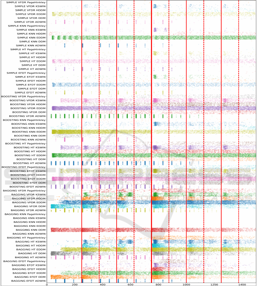
Figure 2: Evaluation of drift detection on Weather based data streams for different model/detector setups. Red lines mark

change points (thin: virtual drift, thick: real drift), and dashed lines mark the end of considered windows. Points mark found

drifts, x-axis shows timepoint/sample number in the stream of detection, y-axis shows setup and run.

ICPRAM 2023 - 12th International Conference on Pattern Recognition Applications and Methods

172

Table 1: Mean F1-score (200 runs) of real drift detection.

Method Elec Forest RBF SEA STAGGER Weather

BAGGING HT HDDM 0.49±0.19 0.23±0.28 0.47±0.36 0.00±0.07 0.99± 0.09 0.48±0.21

KNN DDM 0.18±0.04 0.17±0.07 0.19±0.05 0.19±0.08 0.74± 0.22 0.18±0.05

BOOSTING EFDT KSWIN 0.24±0.06 0.15±0.14 0.28±0.12 0.10±0.22 0.81± 0.25 0.25±0.06

HT ADWIN 0.11±0.13 0.03±0.10 0.16±0.12 0.01±0.05 0.15± 0.18 0.15±0.12

KSWIN 0.23±0.05 0.20±0.16 0.26±0.10 0.11±0.25 0.86± 0.20 0.23±0.05

VFDR KSWIN 0.26±0.06 0.21±0.18 0.27±0.10 0.10±0.22 0.83± 0.20 0.24±0.05

SIMPLE VFDR ADWIN 0.17±0.25 0.01±0.10 0.11±0.23 0.00±0.00 0.52± 0.16 0.16±0.25

KSWIN 0.73±0.33 0.13±0.30 0.43±0.46 0.00±0.07 0.99± 0.10 0.52±0.36

ShapeDD (unsupervised) 0.36±0.25 0.29±0.23 0.45±0.14 0.35±0.08 0.49± 0.14 0.41±0.20

Table 2: Mean number of alerts in stream blocks (200 runs). In block ordering is non-drifting (max. 7), real drift (max. 1),

virtual drift (max. 4).

Method Elec Forest RBF SEA STAGGER Weather

BAGGING HT HDDM 1.03 0.98 1.46 1.06 0.48 1.58 0.56 0.72 0.90 0.01 0.00 0.01 0.02 1.00 0.00 0.88 0.92 1.62

KNN DDM 5.38 0.96 3.58 5.34 0.96 3.62 5.24 0.95 3.56 3.98 0.90 3.32 0.44 1.00 0.38 5.20 0.99 3.54

BOOSTING EFDT KSWIN 3.90 0.98 2.93 3.68 0.64 2.39 2.77 0.87 2.43 1.12 0.21 0.70 0.33 0.96 0.17 3.85 1.00 2.98

HT ADWIN 3.91 0.42 1.97 2.50 0.11 1.42 4.08 0.64 2.06 1.74 0.05 1.06 2.59 0.50 1.50 4.30 0.66 2.13

KSWIN 4.00 1.00 2.92 2.69 0.66 2.28 3.16 0.98 2.84 0.86 0.16 0.70 0.31 1.00 0.19 3.82 1.00 3.24

VFDR KSWIN 3.53 0.99 2.74 2.28 0.64 2.24 2.98 0.94 2.70 0.88 0.20 0.69 0.34 1.00 0.27 3.50 0.99 2.96

SIMPLE VFDR ADWIN 1.03 0.32 0.75 0.44 0.02 0.34 1.06 0.18 0.70 0.04 0.00 0.04 1.10 0.94 0.78 1.25 0.30 0.72

KSWIN 0.27 0.84 0.32 0.26 0.18 0.50 0.18 0.50 0.44 0.00 0.01 0.00 0.00 0.99 0.00 0.30 0.74 0.90

ShapeDD (unsupervised) 0.21 0.72 2.10 0.14 0.66 2.52 0.14 1.00 2.65 0.04 0.97 3.64 0.18 1.00 2.21 0.18 0.86 2.34

drifts. We consider the following drift detectors: AD-

WIN (Bifet and Gavaldà, 2007), DDM (Gama et al.,

2004), EDDM (Baena-García et al., 2006), HDDM-

A (Frías-Blanco et al., 2015), KSWIN (Raab et al.,

2019), and PageHinkley (Page, 1954).

We present the total number of found drift events

per run in Figure 1a and the rate of false alarms in Fig-

ure 1b, where we consider an alarm as a true positive

if it was observed during the ﬁrst

125

samples after the

drift. If it was observed before, i.e., when train and test

distribution coincide, or with a very large delay, i.e.,

after more than 125 into the second part of the stream,

the detection is considered to be a false positive. We

allow multiple true positives per stream. If a stream

does not result in a single detection it is excluded from

the alarm rate analysis.

As can be seen, most of the methods do not yield

any alarms. The ones that do (ADWIN, KSWIN, and

EDDM) show strong variation in the false alarm rate,

where KSWIN outperforms the others in this regard.

Only with respect to the sensitivity in the case of vir-

tual drift, it is outperformed by EDDM due to the low

detection rate. Furthermore, virtual drift is harder to de-

tect than real which is harder than both. Additionally,

except for KSWIN, all methods show an extremely

high false alarm rate.

Drift Detection in a Streaming Setup. To evalu-

ate the decision capabilities in a more realistic setup,

we proceed as follows: We make use of standard, ac-

tive stream learning algorithms and document the time

when the internal drift detectors initiate a model re-

set. We consider both single model approaches (SIM-

PLE), where only a single model is used, and ensem-

ble approaches, including bagging (BAGGING) and

boosting (BOOSTING). We make use of the same

drift detectors as before and consider the following

models: Hoeffding Tree (HT; Bifet et al., 2010), Slid-

ing Window

-NN (KNN; Montiel et al., 2018), Ex-

tremely Fast Decision Trees (EFDT; Manapragada

et al., 2018), and Very Fast Decision Rules (VFDR;

Kosina and Gama, 2013). To verify our claim that

unsupervised drift detectors can help to identify the

change points, we also consider the Shape-based Drift

Detector (ShapeDD; Hinder et al., 2021).

We apply those methods to streams which are con-

structed as follows: Each stream consists of 6 blocks

consisting of 250 datapoints, each from a single dis-

tribution with drift between consecutive blocks. The

distributions are constructed as described above – each

stream is constructed based on a single dataset. Except

for the change from block 1 to 2 and 3 to 4, all blocks

have virtual drift only, from 1 to 2 there is no drift,

from 3 to 4 there is virtual and real drift.

We report the mean F1-score (Table 1) and the

On the Hardness and Necessity of Supervised Concept Drift Detection

173

Figure 3: Effect of alarm rate on model accuracy.

-axes

shows reset frequency in samples between resets,

-axis

shows mean interleaved test-train accuracy over 200 runs.

mean number of alerts per drift type (Table 2) for a

selection of method combinations and ShapeDD. We

split each of the 6 blocks into a ﬁrst and second half

and accumulate the detection in each half block. The

ﬁrst half of the 4th block which corresponds to the

real drift is considered as a positive, all others are as

negatives. Furthermore, we visualized the results on

the stream based on the Weather dataset in Figure 2.

Considering Figure 2, it can be seen that many

drift detectors produce far too many alarms, which

ﬁts the expectation of the ﬁrst experiment. In some

cases, the found drifts seem to be nearly independent

of the actual drift events. Only KSWIN shows a solid

performance in all setups. Furthermore, the SIMPLE

setup produces far fewer drift events, which is to be

expected as they make use of a single drift detector

only. These results are conﬁrmed on the additional

datasets. As one can see in Table 1, for most super-

vised drift detectors we observe low F1-scores. As

can be seen in Table 2, this is caused by high false

positive rates. Indeed, as can easily be seen, many

methods also detect drift in the non-drifting blocks.

In contrast, we observe that the unsupervised drift

detection method ShapeDD obtains comparably high

F1-scores even though false alarms are expected, i.e.,

in case of a perfect unsupervised detection the obtain

F1-score is

0.33

. Reconsidering Table 2, ShapeDD

usually shows the lowest number of detection in non-

drifting blocks. The only exceptions are SEA, where

the other methods with low non-drifting defections do

not detect anything, and STAGGER, which appears to

be a particularly simple dataset for all stream-learning

methods. This perfectly aligns with the theoretical con-

siderations (Corollary 1) and supports our proposal to

combine unsupervised drift detection with a suitable

statistical test to perform supervised drift detection

rather than a loss-based approach.

Effect of False Alarms on Performance. To study

the effect of many false alarms, we used the same

datasets as before to create streams of a length of

1,000

samples without drift. We apply Hoeffding Tree (Bifet

et al., 2010), Sliding Window

-NN (Montiel et al.,

2018), and Very Fast Decision Rules (Kosina and

Gama, 2013) to each of the streams, reset the model

after every

100

150

200

250

300

400

500

600

750

900

, and

1,000

samples, respectively,

to simulate different false alarm rates, and document

the interleaved test-train error. We repeat the process

200

times. The results are shown in Figure 3. As ex-

pected, mean accuracy grows anti-proportionally to

the number of resets (Spearman’s ρ, p < 0.001).

Also, observe that after 200 samples nearly all

methods reach a plateau which justiﬁes the choice of

this sample size in the other experiments.

5 CONCLUSION

In this work, we considered the interconnection of

concept drift, statistical tests, and learning algorithms

from a theoretical point of view. We provided a gen-

eralized notion of real drift and showed that, other

than in the unsupervised setup, a universal supervised

drift detector cannot exist. Considering loss-based su-

pervised drift detection we found that the connection

between real drift and learning models is not valid if

we do not make assumptions about the distributions. In

particular, this approach is not suited for monitoring se-

tups. In our experimental evaluation, we demonstrated

that unsupervised drift detection constitutes a good

choice for this setting. When applying online learning

without additional knowledge guiding the choice of a

suitable model, considering drift detection on the joint

distribution might be a valuable option. Besides, we

found that updating the model very frequently due to

false alarms is decreasing the performance of online

learners. For practical applications, this indicates, that

one should carefully select a suitable model according

to the data.

REFERENCES

Agrawal, R., Imielinski, T., and Swami, A. N. (1993).

Database mining: A performance perspective. IEEE

Trans. Knowl. Data Eng., 5:914–925.

Baena-García, M., Campo-Ávila, J., Fidalgo-Merino, R.,

Bifet, A., Gavald, R., and Morales-Bueno, R. (2006).

Early drift detection method.

Bifet, A. and Gavaldà, R. (2007). Learning from time-

changing data with adaptive windowing. In Proceed-

ings of the Seventh SIAM International Conference on

Data Mining, April 26-28, 2007, Minneapolis, Min-

nesota, USA, pages 443–448.

Bifet, A., Holmes, G., Kirkby, R., Pfahringer, B., and Braun,

ICPRAM 2023 - 12th International Conference on Pattern Recognition Applications and Methods

174

M. (2010). Moa: Massive online analysis. Journal of

Machine Learning Research 11: 1601-1604.

Blackard, J. A., Dean, D. J., and Anderson, C. W. (1998).

Covertype data set.

Bu, L., Alippi, C., and Zhao, D. (2016). A pdf-free change

detection test based on density difference estimation.

IEEE transactions on neural networks and learning

systems, 29(2):324–334.

Ditzler, G., Roveri, M., Alippi, C., and Polikar, R. (2015).

Learning in nonstationary environments: A survey.

IEEE Comp. Int. Mag., 10(4).

Eliades, D. G. and Polycarpou, M. M. (2010). A Fault

Diagnosis and Security Framework for Water Systems.

IEEE Transactions on Control Systems Technology,

18(6):1254–1265.

Elwell, R. and Polikar, R. (2011). Incremental learning of

concept drift in nonstationary environments. IEEE

Transactions on Neural Networks, 22(10):1517–1531.

Frías-Blanco, I., d. Campo-Ávila, J., Ramos-Jiménez, G.,

Morales-Bueno, R., Ortiz-Díaz, A., and Caballero-

Mota, Y. (2015). Online and non-parametric drift de-

tection methods based on hoeffding’s bounds. IEEE

Transactions on Knowledge and Data Engineering,

27(3):810–823.

Gama, J., Medas, P., Castillo, G., and Rodrigues, P. P. (2004).

Learning with drift detection. In Advances in Artiﬁcial

Intelligence - SBIA 2004, 17th Brazilian Symposium

on Artiﬁcial Intelligence, São Luis, Maranhão, Brazil,

September 29 - October 1, 2004, Proceedings, pages

286–295.

Gama, J. a., Žliobait

e, I., Bifet, A., Pechenizkiy, M., and

Bouchachia, A. (2014). A survey on concept drift

adaptation. ACM Comput. Surv., 46(4):44:1–44:37.

Gonçalves Jr, P. M., de Carvalho Santos, S. G., Barros, R. S.,

and Vieira, D. C. (2014). A comparative study on con-

cept drift detectors. Expert Systems with Applications,

41(18):8144–8156.

Gözüaçık, Ö., Büyükçakır, A., Bonab, H., and Can, F. (2019).

Unsupervised concept drift detection with a discrimi-

native classiﬁer. In Proceedings of the 28th ACM in-

ternational conference on information and knowledge

management, pages 2365–2368.

Gretton, A., Borgwardt, K., Rasch, M., Schölkopf, B., and

Smola, A. (2006). A kernel method for the two-sample-

problem. volume 19.

Hanneke, S., Kanade, V., and Yang, L. (2015). Learning with

a drifting target concept. In Int. Conf. on Alg. Learn.

Theo, pages 149–164. Springer.

Harries, M., cse tr, U. N., and Wales, N. S. (1999). Splice-2

comparative evaluation: Electricity pricing. Technical

report.

Hinder, F., Artelt, A., and Hammer, B. (2019). A probability

theoretic approach to drifting data in continuous time

domains. arXiv preprint arXiv:1912.01969.

Hinder, F., Artelt, A., and Hammer, B. (2020). Towards

non-parametric drift detection via dynamic adapting

window independence drift detection (dawidd). In

ICML.

Hinder, F., Brinkrolf, J., Vaquet, V., and Hammer, B. (2021).

A shape-based method for concept drift detection and

signal denoising. In 2021 IEEE Symposium Series

on Computational Intelligence (SSCI), pages 01–08.

IEEE.

Hinder, F., Vaquet, V., and Hammer, B. (2022). Suitability of

different metric choices for concept drift detection. In

International Symposium on Intelligent Data Analysis,

pages 157–170. Springer.

Hu, H., Kantardzic, M., and Sethi, T. S. (2020). No free

lunch theorem for concept drift detection in streaming

data classiﬁcation: A review. WIREs Data Mining and

Knowledge Discovery, 10(2):e1327.

Kosina, P. and Gama, J. (2013). Very fast decision rules

for classiﬁcation in data streams. Data Mining and

Knowledge Discovery, 29:168–202.

Losing, V., Hammer, B., and Wersing, H. (2015). Interactive

online learning for obstacle classiﬁcation on a mobile

robot. In 2015 international joint conference on neural

networks (ijcnn), pages 1–8. IEEE.

Lu, J., Liu, A., Dong, F., Gu, F., Gama, J., and Zhang, G.

(2018). Learning under concept drift: A review. IEEE

Transactions on Knowledge and Data Engineering,

31(12):2346–2363.

Manapragada, C., Webb, G. I., and Salehi, M. (2018). Ex-

tremely fast decision tree. In Proceedings of the 24th

ACM SIGKDD International Conference on Knowl-

edge Discovery & Data Mining, pages 1953–1962.

Mohri, M. and Muñoz Medina, A. (2012). New analysis and

algorithm for learning with drifting distributions. In Int.

Conf. on Alg. Learn. Theo, pages 124–138. Springer.

Montiel, J., Read, J., Bifet, A., and Abdessalem, T. (2018).

Scikit-multiﬂow: A multi-output streaming framework.

Journal of Machine Learning Research, 19(72):1–5.

Page, E. S. (1954). Continuous inspection schemes.

Biometrika, 41(1-2):100–115.

Pedregosa, F., Varoquaux, G., Gramfort, A., Michel, V.,

Thirion, B., Grisel, O., Blondel, M., Prettenhofer, P.,

Weiss, R., Dubourg, V., Vanderplas, J., Passos, A.,

Cournapeau, D., Brucher, M., Perrot, M., and Duch-

esnay, E. (2011). Scikit-learn: Machine learning

in Python. Journal of Machine Learning Research,

12:2825–2830.

Raab, C., Heusinger, M., and Schleif, F.-M. (2019). Reac-

tive soft prototype computing for frequent reoccurring

concept drift. In ESANN.

Shah, R. D. and Peters, J. (2020). The hardness of condi-

tional independence testing and the generalised covari-

ance measure. The Annals of Statistics, 48(3):1514–

1538.

Shalev-Shwartz, S. and Ben-David, S. (2014). Understand-

ing machine learning: From theory to algorithms.

Cambridge university press.

Street, W. N. and Kim, Y. (2001). A streaming ensemble

algorithm (SEA) for large-scale classiﬁcation. In Pro-

ceedings of the seventh ACM SIGKDD international

conference on Knowledge discovery and data mining,

San Francisco, CA, USA, August 26-29, 2001, pages

377–382.

Vaquet, V., Menz, P., Seiffert, U., and Hammer, B. (2022).

Investigating intensity and transversal drift in hyper-

spectral imaging data. Neurocomputing, 505:68–79.

Webb, G. I., Lee, L. K., Petitjean, F., and Goethals, B. (2017).

Understanding concept drift. CoRR, abs/1704.00362.

On the Hardness and Necessity of Supervised Concept Drift Detection

175