Using Balancing Methods to Improve Glycaemia-Based Data Mining

Diogo Machado

1,3

, Vítor Santos Costa

2,3

and Pedro Brandão

1,3

Instituto de Telecomunicações, Portugal

INESC-TEC, Portugal

Faculty of Science of the University of Porto, Portugal

Keywords:

Data Mining, Diabetes, Data-Balance, over-Sampling, Under-Sampling.

Abstract:

Imbalanced data sets pose a complex problem in data mining. Health related data sets, where the positive class

is connected to the existence of an anomaly, are prone to be imbalanced. Data related to diabetes management

follows this trend. In the case of diabetes, patients avoid situations of hypo/hyperglycaemia, which is the

anomaly we want to detect. The use of balancing methods can provide more examples of the minority class, and

assist the classiﬁer by clearing the decision boundary. Nevertheless, each over-sampling and under-sampling

method can affect the data set uniquely, which will inﬂuence the classiﬁer’s performance. In this work, the

authors studied the impact of the most known data-balancing methods applied to the Ohio and St. Louis

diabetes related data sets. The best and most robust approach was the use of ENN with SMOTE. This hybrid

method produced signiﬁcant performance gains on all the performed tests. ENN in particular had a meaningful

impact on all the tests. Given the limited volume of glycaemia-based data available for diabetes management,

over-sampling methods would be expected to have a greater role in improving the classiﬁer’s performance. In

our experiments, the clearing of noise values by the under-sampling methods, produced better results.

1 INTRODUCTION

Data mining can be regarded as the computational pro-

cess that analyses and extracts knowledge from a data

set (Raval, 2012). Data mining has contributed posit-

ively in many health-domains such as liver diseases,

cardiovascular diseases, coronary diseases, cancer, and

diabetes (Shukla et al., 2014).

In this work we focus on data mining applied to

diabetes. This chronic disease, characterised by high

glycaemia levels (blood glucose), affected 463 million

people around the world in 2019, and it is projected

to reach 700 million by 2045 (International Diabetes

Federation, 2019).

Diabetic patients should have a strict manage-

ment of their disease to avoid both hyperglycaemia

(very high glycaemia levels) and hypoglycaemia (very

low glycaemia levels). Both can lead to severe con-

sequences. In the long term, repeated hyperglycaemia

episodes damage the large and small blood vessels,

and may lead to blindness, heart problems, increased

risk of having a stroke, among other serious health

issues. In the short term, extreme hyperglycaemia and

hypoglycaemia events can make the person go into a

coma, and even death (Mouri and Badireddy, 2021;

Seery, 2019b,a).

Given the severity of these occurrences, most dia-

betic patients attempt, to their best ability, to stay

within a glycaemia range considered normal. There-

fore, in data mining approaches, the data sets have an

imbalance, as most observations will be normal. Im-

balanced data is common in health related data sets,

where the data target consists of values that are either

designated as "normal" or "abnormal" (Li et al., 2010).

This reality causes the use of data mining algorithms

to be more complex, since data imbalances cause bias

towards the majority class (Li et al., 2010).

Glucose values were traditionally obtained only

through ﬁnger-pricking. This invasive method, accord-

ing to medical doctors, should be performed at least

six times per day, before and after the three main meals

(breakfast, lunch, and dinner). Due to the small num-

ber of samples, using ﬁnger-based glucose values for

data mining is challenging.

Nowadays, diabetic patients have a more conveni-

ent method of glycaemia tracking, continuous-glucose

monitoring (CGM). CGM uses a painless, one-time

sensor device application under the skin of the belly

or the back of the arm, that must be replaced period-

ically (around every seven to ten days). While less

188

Machado, D., Costa, V. and Brandão, P.

Using Balancing Methods to Improve Glycaemia-Based Data Mining.

DOI: 10.5220/0011797100003414

In Proceedings of the 16th International Joint Conference on Biomedical Engineering Systems and Technologies (BIOSTEC 2023) - Volume 5: HEALTHINF, pages 188-198

ISBN: 978-989-758-631-6; ISSN: 2184-4305

 2023 by SCITEPRESS – Science and Technology Publications, Lda. Under CC license (CC BY-NC-ND 4.0)

convenient, the traditional ﬁnger-prick method is more

accurate than CGM (Siegmund et al., 2017; Cengiz and

Tamborlane, 2009; Medtronic Diabetes, 2014). This is

a consequence of the physiological delay between in-

terstitial glucose and blood-glucose (Cengiz and Tam-

borlane, 2009). Even so, CGM devices are able to

sample a new glycaemia value each ﬁve minutes, with

some devices having an even higher sample rate. This

amount of data would, realistically, be impossible to

obtain using the traditional ﬁnger-pricking method. In

terms of data mining, CGM devices can give a better

perspective of the diabetic patient’s glycaemia val-

ues and trends throughout the day. While more data

is beneﬁcial, CGM data continues to be imbalanced.

Data balancing methods are often used to improve

learning performance. In this work, we study how

different methods perform on two different data sets.

The ﬁrst reports ﬁnger-prick-based glycaemia data,

the second reports CGM-based glycaemia. Although

CGM is now prominent in data mining, having both

types of glycaemia sampling methods as target will

allow a better evaluation of the impact of data balan-

cing (Machado et al., 2022).

Given the scope of this work, we decided to limit

the number of classiﬁcation methods, to broaden the

number of data balancing method variations. For the

classiﬁcation of glycaemia values, we chose the Ran-

dom Forest (RF) ensemble learning method. RF allows

the evaluation of the balancing method’s effects, but

also the assessment of the impact of different features.

The article starts with a brief presentation and stat-

istics of the used data sets; it follows with an explana-

tion of the data balance methods present in this work;

after we discuss the few articles of related work; we

then describe the experiments’ and their results; and

ﬁnally, we present the work’s conclusions.

2 DATA SETS

In this work, two very distinct data sets were used to

evaluate different balancing techniques.

The data set from the University of St. Louis, avail-

able on the UCI Machine Learning Repository (Dua

and Graff, 2017)

contains data from 70 different pa-

tients, over several weeks to months (minimum eight

days, maximum 288 days). This data set possesses

data concerning the patient’s glycaemia values (ob-

tained through ﬁnger-prick testing), insulin adminis-

tration (short, medium, and long duration), and meal

and exercise classiﬁcations (regular, more-than-usual

or less-than-usual quantities). In terms of total records,

https://archive.ics.uci.edu/ml/datasets/diabetes

the St. Louis data set has 11737 ﬁnger-prick-based

glycaemia records, 317 meal records, 8110 insulin

administration records, and 201 exercise records. In

terms of glycaemia record variance, the minimum num-

ber of records by a single user in the data set is 25

and the maximum is 616. Regarding the glycaemia

value classiﬁcation: 11.62% of values represent hy-

poglycaemia; 14.51% represent hyperglycaemia; and

ﬁnally 73.87% of the values are considered as normal.

The Ohio data set (Marling and Bunescu, 2020)

contains eight weeks of data from 12 different pa-

tients. This data set possesses both sensor (continuous

monitoring) and ﬁnger-prick tested glycaemia values,

administrated insulin dosages (basal and regular), exer-

cise, and other physiological parameters e.g. the heart

rate, for patients that used a proper sensor. The Ohio

data set has a total of 166533 sensor-based glycaemia

records, 4566 ﬁnger-prick-based glycaemia records,

2773 meal records, 3731 insulin records, and 221 ex-

ercise records. This considerable amount of records,

compared to the St. Louis data set, occurs because

the CGM device used by the patients automatically

recorded a new glycaemia value every ﬁve minutes.

In terms of glycaemia value classiﬁcation, the values

must be divided, having into account the glycaemia

sampling method (ﬁnger or sensor-based). In terms

of glycaemia values that were obtained through a

continuous monitor (sensor): 3.28% of values repres-

ent hypoglycaemia; 8.48% represent hyperglycaemia;

and, ﬁnally, 88.23% of the values are considered as

normal. Regarding the glycaemia values, obtained

through ﬁnger-pricking: 4.58% of values represent hy-

poglycaemia; 12.07% represent hyperglycaemia; and,

ﬁnally, 83.36% of the values are considered as normal.

While the St. Louis data set contains fewer fea-

tures and sparser data, the Ohio data set is richer and

contains continuous glycaemia data from a glycaemia

sensor. Figures 1 to 3 display statistics about: the pa-

tient’s ID, the number of days recorded, number of

hypoglycaemia, number of normal glycaemia, number

of hyperglycaemia, and the HbA1c correspondent to

the glycaemia values recorded. Considering the in-

formation in these ﬁgures, the patients that constitute

St. Louis data set seem to have glycaemia values less

controlled than the ones present in the Ohio data set.

The St. Louis data set contains, in percentage, more

hypoglycaemia and hyperglycaemia. Although the

level of HbA1c seems on par with the Ohio data set,

the high standard deviation refutes this idea.

The referred data sets contain raw records. The two

data sets used in this work result from preprocessing

the St. Louis and Ohio data sets and have different

targets and features. The ﬁrst generated data-set targets

ﬁnger-based glycaemia. It concatenates the St. Louis

Using Balancing Methods to Improve Glycaemia-Based Data Mining

189

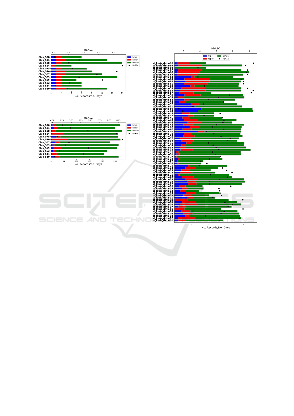
Figure 1: Ohio raw ﬁnger-prick based glycaemic data statist-

ics.

Figure 2: Ohio raw sensor-based glycaemic data statistics.

and the Ohio data sets, and it is restricted to the more

limited set of available features in the S Louis data.

The second data-set targets CGM-based glycaemia,

only available in the Ohio data set.

The Ohio-St. Louis joint data set, with ﬁnger-prick

glycaemia as target, is composed of 43 features. Of

these, three of them are parameters commonly used

by medical doctors to evaluate the patients’ diabetes

management.

The time-in-range represents the number of gly-

caemia records within the range of [70-180] divided by

the total amount of glycaemia records. Values of time-

in-range above 0.7 (70%) are considered good. The

glycaemia value tendency is a metric that represents

the general tendency of the glycaemia values. This

parameter is specially important when the glycaemia

values are reaching hypo/hyperglycaemia thresholds.

To calculate this parameter, the authors utilised the

least square polynomial regression. The variation

coefﬁcient represents the standard value deviation di-

vided by the value average, then multiplied by 100.

This coefﬁcient is more used than the standard devi-

ation parameter since it is less dependent of the average

value. In terms of glycaemia value management, the

variation coefﬁcient should be below 36%.

The features present in the conjunct data set are

the glycaemia designation classiﬁed as: hypergly-

caemia (glycaemia values above 250), hypoglycaemia

(glycaemia values under 70), and normal (glycaemia

values between 70 and 250); the weekday and time

of day of the target glycaemia; past ﬁnger-based

Figure 3: St. Louis ﬁnger-prick glycaemic data statistics.

glycaemia value, time in range, tendency, variation

coefﬁcient, average, and the existence of prior hypo-

/hyperglycaemia. These features are sampled in differ-

ent time intervals: 30 minutes to one hour, one to three

hours, three to 12 hours, 12 to 24 hours, and 24 to 48

hours. We calculate the existence of recorded meals in

the last three hours, and in the last three to six hours;

the existence of recorded insulin bolus in the last hour,

in the last hour to three hours, in the last three to six

hours, and in the last six to 12 hours; the existence of

recorded exercises in the last hour. These features are

displayed in Listing: 1.

The Ohio sensor-based data set is composed of 81

features, the 43 already present in the Ohio-St. Louis

conjunct data set, 33 features related to sensor-based

glycaemia values, and ﬁve new features. The new fea-

tures contain information not available in the St. Louis

data set: if the user paused, reduced or increased the

basal insulin; the correlation between recorded carbo-

hydrates and the insulin bolus; and the physical efforts

HEALTHINF 2023 - 16th International Conference on Health Informatics

190

glycaemia_designation , wee kday ,

time _day ,

fin g e r _ g l y c a e mia _ v a l u e _ 3 0 m _1h , [.. .] ,

fin g e r _ t i m e _ i n _ r ang e _ 3 0 m _ 1 h , [...] ,

finger_te n d e n c y _ 3 0 m _ 1 h , [.. .] ,

fin g e r _ v a r i a t i o n _co f _ 3 0 m _ 1 h , [...] ,

finger_average_30m_1h , [.. .] ,

finger _ h a d _ h y p e r _ 3 0 m _ 1 h , [...] ,

finger_ha d _ h y p o _ 3 0 m _ 1 h , [.. .] ,

had_meal_last _ 3 h , h a d _ meal_3h_6h ,

had_insulin_last_1h , [... ] ,

ex e r c i s e _ l a st _ 1 h

Listing 1: Part of the features in the Ohio-St. Louis joint data

set.

detected. Efforts are an experimental measure, calcu-

lated by the authors through the heart rate information

present on the Ohio data set. The features present on

the Ohio sensor-based data set are displayed in List-

ing: 2.

glycaemia_designation , wee kday ,

time _day ,

glycaemia _ v a l u e _ 3 0 m _ 1 h , [.. .] ,

time_in_range_30m_1h , [ ...] ,

tendency_30 m _ 1 h , [.. .] ,

average_3 0 m _ 1 h , [ ...] ,

variation_cof_30m_1h , [ ...] ,

had_hyper_30m _ 1 h , [...] ,

had_hypo_30 m _ 1 h , [.. .] ,

fin g e r _ g l y c a e mia _ v a l u e _ 3 0 m _1h , [.. .] ,

fin g e r _ t i m e _ i n _ r ang e _ 3 0 m _ 1 h , [...] ,

finger_te n d e n c y _ 3 0 m _ 1 h , [.. .] ,

fin g e r _ v a r i a t i o n _co f _ 3 0 m _ 1 h , [...] ,

finger_average_30m_1h , [.. .] ,

finger _ h a d _ h y p e r _ 3 0 m _ 1 h , [...] ,

finger_ha d _ h y p o _ 3 0 m _ 1 h , [.. .] ,

n_basal_paused_1h_3h ,

n_basal_reduced_1h_3h ,

n_basa l _ i n c r e a s e d _ 1 h _ 3 h ,

ca r b s _ i n s u l in_ c o r r e l a t i on _ 1 h _ 3 h ,

had_meal_last _ 3 h , h a d _ meal_3h_6h ,

had_insulin_last_1h , [... ] ,

exercise_last _ 1 h ,

eff o r t _ l a s t _ 1 h

Listing 2: Part of the features in the Ohio data set.

3 DATA BALANCING METHODS

Glycaemia-based data is particularly imbalanced. Tak-

ing the St. Louis data set as an example, the hy-

poglycaemia values represent only 10% of the total

values, and the hyperglycaemia values represent 13%,

leaving the denominated normal values to represent

77% of the data set’s glycaemia values. This trend,

also visible in the Ohio data set, should be expected,

given that both hypoglycaemia and hyperglycaemia

values represent health risks that should be prevented

by patients.

Imbalanced data sets are a known problem in data-

mining. A common approach is the use of over-

sampling and/or under-sampling, to achieve some sort

of balance within the data set’s classes.

3.1 Over-Sampling Methods

Over-sampling is a method that produces new values

in order to increase the representation of the minor-

ity classes. There are two base approaches to over-

sampling: by value duplication, and by creating syn-

thetic values. Value duplication can virtually balance

the weight of every class, but since each new value

does not include additional information to the model,

it can create value bias. Within the over-sampling

methods, that create synthetic values, there are some

different approaches to consider:

Synthetic Minority Oversampling TEchnique

(

SMOTE

) (Bowyer et al., 2011): This technique man-

ufactures values similar to the ones already present

in the imbalanced class using the k-Nearest Neigh-

bours (

KNN

) algorithm. To achieve this,

SMOTE

chooses a random value, from the minority class, and

k of the nearest neighbours. The method then creates

synthetic values within the chosen values’ domain.

Borderline-SMOTE (Han et al., 2005): Classiﬁers’

decisions are dependant of the clarity of the decision

border. The line that divides and enables classiﬁc-

ation is present where values from different classes

congregate. The values in this location implicitly as-

sume a greater importance in the data set. While the

SMOTE

method creates values at random positions,

the Borderline-SMOTE chooses, at random, values

close to the border between classes to run the

SMOTE

value creation method.

Borderline-SMOTE SVM (Nguyen et al., 2011):

Similar to Borderline-SMOTE, this method, instead of

KNN

, uses Support-Vector Machine (

SVM

) to choose

values at the decision border. Additionally, this method

selects regions in the minority class that have less value

density. The method then creates values towards the

class boundary.

Adaptive Synthetic Sampling (

ADASYN

) (He et al.,

2008): It is a more generalised form of the

SMOTE

method. The main difference between these methods

is the use of the density distribution. This method

searches low density data areas, in minority classes,

and uses these empty spaces to generate synthetic val-

ues. It re-shapes the decision boundary, using syn-

thetic values, according to their learning difﬁculty

level. More data will be generated for classes that

Using Balancing Methods to Improve Glycaemia-Based Data Mining

191

are harder to learn.

3.2 Under-Sampling Methods

Contrary to over-sampling, under-sampling method

achieves class equilibrium by excluding values in the

majority class. This sampling can be done at ran-

dom, by removing random values until the classes

have equal weight, or it can be done while aware of

the removed values. Some known, and used, under-

sampling methods are:

Near-Miss Under-Sampler: It is a collection of under-

sampling methods based on the work of Mani and

Zhang (2003), and available on the imblearn library

that uses

KNN

to select examples from the majority

class. Near-Miss has three versions:

•

NearMiss-1 retains values with the minimum av-

erage distance to the three closest minority class

values;

•

NearMiss-2 retains values with the minimum av-

erage distance to the three furthest minority class

values;

•

NearMiss-3 retains values with the minimum dis-

tance to each minority class value.

Condensed Nearest Neighbors (

CNN

) Rule Under-

Sampling (Hart, 1968):

CNN

algorithm uses the one

nearest neighbour rule to decide, at each sample, if a

sample should be added or removed from the data set.

The

CNN

algorithm creates a sub-set containing all the

minority class values, and a sample from the majority

class. Then, the values from the majority class are

iterated and classiﬁed, using the current sub-set and

the one nearest neighbour rule. The samples that are

not correctly classiﬁed from the majority class set, are

added to the sub-set. In the end, this method is able

to obtain a sub-set containing all the minority class

values and the inconsistent majority class values.

Tomek-links for Under-Sampling (Tomek et al.,

1976): Based on

CNN

, Tomek-links addresses two

lacking elements of the

CNN

method, according to the

author. The ﬁrst point that was criticised by Tomek

et al. (1976) was the fact that the values, at the be-

ginning of the

CNN

method, are chosen at random.

Only later in the process, does the method become

less random and collects values closer to the decision

boundary. This process returns a sub-set containing

redundant samples, that could be eliminated. The pro-

posed solution is to ﬁnd links between pair values of

different classes that, together, have the smallest Eu-

clidean distance. This method can be used to erase

possible ambiguous values by ﬁnding and removing

examples in the majority class, that are closest to the

minority class. This action clears the borderline area

and facilitates class division.

Edited Nearest Neighbors (

ENN

) Rule for Under-

Sampling (Wilson, 1972): This method for re-

sampling and classiﬁcation can be used as an under-

sampling method. This method uses

KNN

to identify

and remove incoherent values in the data set. The pro-

cess begins with a set equal to the training set. Each

value in this set is compared to its neighbours using

KNN

method, by default with k equal to three. If

the selected value differs from the majority, then the

value is removed. Similarly to Tomek-links, the

ENN

rule for under-sampling removes noisy and ambigu-

ous values from the class boundary, thus supporting

classiﬁcation methods.

3.3 Joint Methods

One-Sided Selection for Under-Sampling

(OSS) (Kubat et al., 1997): This method com-

bines the Tomek-links and the

CNN

method. The

Tomek-links method is used as an under-sampling

method to remove noisy and borderline values from

the majority class. The

CNN

method is used to

remove values from the majority class that are distant

from the decision border.

Neighbourhood Cleaning Rule for Under-Sampling

(NCR): This is an under-sampling method, designed

to prioritise data quality, in detriment of data bal-

ance (Laurikkala, 2001). It combines the

CNN

method

and the

ENN

rule methods to remove redundant noise

values. By removing close border points, this method

is able to smooth the decision boundary (Gu et al.,

2008).

SMOTE and Tomek-links: Batista et al. (2004) pro-

pose the application of SMOTE to balance the data set,

followed by the Tomek-links method. In this proposal,

the Tomek-links method would not be used to under-

sample the majority class. Instead, this method is used

to remove values from every class. By doing this, the

authors claim that this method is capable of producing

a balanced data set, with well-deﬁned class clusters.

SMOTE and

ENN

: Similar to the previous proposal,

Batista et al. (2004) also proposed the use of SMOTE

and

ENN

, instead of the Tomek-links method. They

afﬁrm that, since

ENN

tends to remove more examples

than Tomek-links, it should be expected to obtain a

clearer decision boundary.

The different balancing techniques attempt to reach

a similar goal: to clear the decision boundary and fa-

cilitate the distinction between classes. Over-sampling

techniques, while trying to fulﬁl the previous objective,

focus on increasing the amount of available data on

the minority classes. Unfortunately, there is neither a

HEALTHINF 2023 - 16th International Conference on Health Informatics

192

method, nor a junction of methods, that reigns above

the rest. Depending on the available data, the balan-

cing methods applied will create different impacts.

4 STATE OF THE ART

In recent times, the use of data mining and machine

learning applied to the ﬁeld of diabetes seems to be

focused on glycaemia value and/or hypo or hyper-

glycaemia occurrence prediction. These approaches

mostly use temporal-based approaches that do not re-

quire balancing. Reviewing the blood glucose level

prediction challenge papers of the Knowledge Discov-

ery in Healthcare Data 2020, we found none of the 17

articles to use any type of data balancing.

However, exceptions do exist. The work by Mayo

et al. (2019) uses over-sampling to increase the per-

formance of a machine learning-based method for

short-term glycaemia prediction. In this work ran-

dom over-sampling,

SMOTE

ADASYN

were used.

This work only concludes that there are performance

gains from using over-sampling. It is never mentioned

which balancing approach beneﬁted more the machine

learning method.

The work by Berikov et al. (2022) developed a

machine learning method for the prediction of noc-

turnal hypoglycaemia in hospitalised patients. This

proposal used a personalised approach to both under

and over-sampling. The over-sampling method used

Gaussian noise to introduce new synthetic CGM val-

ues with a nocturnal hypoglycaemia occurrence. The

under-sampling, was used to select records that do

not contain events of nocturnal hypoglycaemia. The

method consisted of a k-medoids algorithm with a

number of clusters equal to the number of nocturnal

hypoglycaemia occurrences. This process then returns

a group of medoids that do not contain nocturnal hy-

poglycaemia events. This methodology is rather un-

usual, as it is composed of a somewhat random over-

sampler, and, for over-sampling, selects a group of

values that do not contain the study’s target. In the

end, the study concluded that the use of sampling was

insigniﬁcant. The authors afﬁrm that the inﬂuence of

data balancing, according to their results, depends on

the machine learning method being applied. They refer

that the use of over-sampling alone resulted on a slight

increase in performance.

Alashban and Abubacker (2020) studied the use

of over-sampling and the joint use of over-sampling

and under-sampling to glycaemia-based data. This

work’s objective is to classify patients as normal, pre-

diabetic, or diabetic. This study does not directly

correlate to diabetes management, nonetheless, it of-

fers a signiﬁcant view on the results of applying dif-

ferent balancing approaches to glycaemia-based data.

The over-sampling methods used in this work were:

random over-sampling, and

SMOTE

. The hybrid ap-

proach tested

SMOTE

with Tomek-link, and

SMOTE

with

ENN

. This study concluded that, although every

sampling technique is better than the use of an im-

balanced data set, the random over-sampling method

achieved better performance gains.

Although existent, the analysis of the impact of

balancing techniques on diabetes management data

is insufﬁcient. The work by Alashban and Abu-

backer (2020) was the more complete study, and even

this study only evaluated four possible approaches to

data balancing.

To have a clearer idea of the real impact of over-

sampling and under-sampling on glycaemia-based

data, we will test the most known methods for over-

sampling and under-sampling, as well as the hybrid

combination of said methods.

5 METHODOLOGY

Balancing data can be approached by applying a single

under-sampling, or over-sampling method, or by ap-

plying both methods. To have a complete depiction

of the impact of the use of balancing methods on dia-

betes’ data, every possible combination of single and

conjunct method was tested, including applying no

balancing methods. In the conjunct method, over-

sampling is applied in order to produce more examples

in the minority classes, and then under-sampling is

applied to ﬁlter the majority class and balance the data

set. The balancing methods were only applied to train-

ing sets. The test set remains imbalanced, to determine

the classiﬁer’s performance with real data.

The classiﬁcation method used to test the impact

of balancing was the random forest.

Random forest is an ensemble learning method

commonly used for classiﬁcation and regression. This

method consists of a collection of decision trees. The

decisions made by this method are obtained through

majority vote of the created decision trees. The ran-

dom forest method was chosen for this work for its

robustness. It inherits from the decision trees method

its scale in-variance, robustness to irrelevant features,

and, contrary to decision trees, random forests tend to

not over-ﬁt as much.

The available data sets are composed by data from

different individuals. To evaluate the impact of each

balancing technique, on individual and on community

sets, two tests were carried out: (i) an individual test,

that applies an 80-20 cut on a single data set and runs

Using Balancing Methods to Improve Glycaemia-Based Data Mining

193

the random forest classiﬁer; (ii) and a leave-one-out

test, that singles out a user to be the test set and estab-

lishes the remaining users’ data as the training set.

To rank the different balancing methods and ap-

proaches, the F1-score was calculated. Although other

metrics are usually also applied in data mining ana-

lysis, F1 is the most commonly used metric in cases

of imbalanced data sets.

Precision is a metric that quantiﬁes the number

of correct positive predictions over all positive pre-

dicted values. The precision metric is represented on

equation 1, where

deﬁnes true positives,

false

positives, and

false negatives. Recall, displayed on

equation 2 quantiﬁes the number of correct positive

predictions over all possible positive predictions. The

F1-score, represented on equation 3 is the precision

and recall’s harmonic mean. Rather than focusing on

pure accuracy, the F1-score focuses on the positive

class, which, in an imbalanced data set, has a greater

impact than accuracy. Higher F1-score values are as-

sociated with a better performance of the model.

P =

+ F

)

(1)

R =

+ F

)

(2)

F1 =

2 ∗ P ∗ R

P + R

(3)

AP =

∑

− R

n−1

(4)

Each data set, for each test, will be divided in three

data sets for binary classiﬁcation, where each class is

set as positive, against the remaining two (negative)

classes. The “normal” class is an exception. Instead

of considering the “normal” class against hypo and

hyperglycaemia, the classes that represent non-normal

glycaemia were set as the positive against the “nor-

mal” class. The F1-score and the F1-score’s standard-

deviation (SD) is then calculated for each set. As an

evaluation metric, the F1-scores of each set are av-

eraged by balancing approach and ordered from best

to worst. This way, it is possible to evaluate the best

approaches on average, and the best approach for a

particular class.

6 RESULTS

As previously mentioned, the following results are

composed of the F1-scores and their respective SD for

the hypoglycaemia focused set, the hyperglycaemia fo-

cused set, and the not normal focused set. In Tables 1,

through 4 these parameters are presented.

The approaches are ordered from best to worst,

considering their hypoglycaemia F1-score and SD.

As previously mentioned, episodes of hypoglycaemia

pose a more immediate and concerning danger than

hyperglycaemia, or other intermediate glycaemia level

states. Considering this fact, it is important to prioritise

hypoglycaemia as the main focus for classiﬁcation.

While the leave-one-out approach encompasses

most of the available data, and it is capable of running

with no issues, some individual sets with ﬁnger-prick-

based glycaemia lack enough data to run balancing

techniques and the random forest classiﬁer. Sensor

data, with a higher volume of data, was able to com-

plete all the individual and the leave-one-out tests.

The balancing methods are displayed from top to

bottom according to their evaluation rank.

The results of the individual tests using ﬁnger-

prick-based glycaemia values as target (displayed on

Table 1) have near miss as the best approach. ENN and

near-miss alone, or used together with over-sampling

methods, constitute nine of the top ten scoring ap-

proaches. In terms of over-sampling approaches, in the

top ten, the adaptive synthetic sampling method was

the most represented, appearing three times, associ-

ated with under-sampling methods. As a sole method,

over-sampling methods achieved poor results, being at

the bottom of the result’s table.

The results of the individual tests using CGM-

based glycaemia values as target (see Table 2) have

the conjunct method, using borderline SMOTE fol-

lowed by ENN, as the best approach. In this test

the ENN dominates the best approaches. As a stan-

dalone method, ENN is ranked fourth. The near miss

approach, which was ﬁrst on the previous test, did

not achieve the same success. Although near miss

with SMOTE rank sixth, the remaining near miss ap-

proaches rank on the bottom half of the results table.

In this test, applying no balancing approaches achieved

the worse results.

The results of the leave-one-out tests using ﬁnger-

prick-based glycaemia values as target are displayed

on Table 3.

As the individual ﬁnger-prick-based results, this

test has the near miss method as the best balancing

approach. The following three best approaches have

ENN as a common denominator. Near miss seems to

falter when applied together with over-sampling. This

fact hints to an inability of the near miss approach

to clear the noise introduced by the over-sampling

methods. In contrast, ENN only has a positive impact

when applied in combination with an over-sampling

method. ENN in this test was inconsistent. While

used with adaptive synthetic sampling, SMOTE, and

borderline SMOTE, ENN achieved very good results,

close to the ones obtained by the top ranking method.

HEALTHINF 2023 - 16th International Conference on Health Informatics

194

Table 1: Data balancing methods results for the individual tests, using data based on the Ohio and St. Louis data sets, sampled

considering ﬁnger-prick-based glycaemia-based values as target.

Under-sample Over-sample

hypo hyper not normal

F1(SD)

near miss 0.20 (0.13) 0.29 (0.16) 0.38 (0.14)

enn smote 0.20 (0.17) 0.35 (0.16) 0.40 (0.18)

enn

borderline svm

smote

0.20 (0.18) 0.22 (0.16) 0.18 (0.17)

enn

adaptive syn-

thetic sampling

0.19 (0.16) 0.28 (0.15) 0.36 (0.18)

enn

borderline smote

0.17 (0.16) 0.28 (0.20) 0.38 (0.20)

. . .

tomek links

borderline svm

smote

0.09 (0.15) 0.16 (0.17) 0.25 (0.16)

smote 0.09 (0.13) 0.16 (0.18) 0.28 (0.20)

no balancing 0.06 (0.13) 0.12 (0.18) 0.22 (0.21)

tomek links 0.06 (0.13) 0.14 (0.19) 0.25 (0.21)

Table 2: Data balancing methods results for the individual tests, using data based on the Ohio data set, sampled considering

CGM-based glycaemia-based values as target.

Under-sample Over-sample

hypo hyper not normal

F1(SD)

enn

borderline smote

0.25 (0.16) 0.55 (0.09) 0.47 (0.08)

enn smote 0.22 (0.14) 0.51 (0.14) 0.42 (0.14)

enn

adaptive syn-

thetic sampling

0.20 (0.15) 0.52 (0.11) 0.41 (0.13)

enn 0.19 (0.15) 0.54 (0.09) 0.46 (0.10)

enn

borderline svm

smote

0.19 (0.15) 0.48 (0.13) 0.38 (0.16)

. . .

near miss

adaptive syn-

thetic sampling

0.10 (0.13) 0.43 (0.16) 0.36 (0.16)

tomek links

borderline svm

smote

0.09 (0.14) 0.46 (0.12) 0.39 (0.13)

no balancing 0.07 (0.10) 0.41 (0.15) 0.34 (0.16)

As a sole approach, ENN is on the bottom half of

the table, being one of the top ﬁve worse approaches.

With borderline SVM SMOTE, ENN even reaches the

bottom of the table, under the no balancing technique.

The results of the leave-one-out tests using CGM-

based glycaemia values as target (displayed on Table 4)

have ENN as the best balancing approach. Apart from

when applied together with borderline SVM SMOTE,

ENN is present in the top four best approaches. Con-

trasting with previous tests, the leave-one-out CGM-

based test had near miss as the worse approach, under

the use of no balancing techniques.

Considering all the obtained results, the method

with greater impact was the ENN under-sampling tech-

nique. This under-sampling method, while used to-

gether with over-sampling, is present on the best ap-

proaches of every test.

In terms of over-sampling as a sole approach, there

Using Balancing Methods to Improve Glycaemia-Based Data Mining

195

Table 3: Data balancing methods’ results for the leave-one-out test, using data based on the Ohio and St. Louis data sets,

sampled considering ﬁnger-prick-based glycaemia-based values as target.

Under-sample Over-sample

hypo hyper not normal

F1(SD)

near miss 0.22 (0.13) 0.28 (0.15) 0.43 (0.16)

enn

adaptive syn-

thetic sampling

0.20 (0.16) 0.29 (0.14) 0.43 (0.16)

enn smote 0.20 (0.16) 0.29 (0.15) 0.43 (0.16)

enn

borderline smote

0.20 (0.16) 0.28 (0.15) 0.43 (0.16)

near miss smote 0.19 (0.20) 0.27 (0.19) 0.38 (0.20)

. . .

tomek links 0.13 (0.22) 0.13 (0.20) 0.22 (0.21)

no balancing 0.13 (0.22) 0.13 (0.21) 0.19 (0.21)

enn

borderline svm

smote

0.13 (0.19) 0.16 (0.17) 0.16 (0.16)

Table 4: Data balancing methods’ results for the leave-one-out test, using data based on the Ohio set, sampled considering

CGM-based glycaemic values as target.

Under-sample Over-sample

hypo hyper not normal

F1(SD)

enn 0.32 (0.13) 0.58 (0.09) 0.52 (0.11)

enn

adaptive syn-

thetic sampling

0.31 (0.13) 0.57 (0.07) 0.50 (0.09)

enn smote 0.31 (0.14) 0.58 (0.08) 0.51 (0.09)

enn

borderline smote

0.30 (0.14) 0.58 (0.08) 0.51 (0.09)

borderline svm

smote

0.28 (0.16) 0.59 (0.08) 0.53 (0.10)

. . .

tomek links 0.26 (0.14) 0.59 (0.08) 0.53 (0.11)

no balancing 0.11 (0.09) 0.57 (0.08) 0.48 (0.11)

near miss 0.11 (0.06) 0.34 (0.13) 0.35 (0.09)

was no clear best method. The creation of synthetic

values, if not ﬁltered, introduces noise and thus, under-

mines the classiﬁer’s results.

Overall the best approach was the use of ENN with

SMOTE. While SMOTE produces synthetic values

that create more training opportunities, the ENN under

sampler clears the decision border for a better clas-

siﬁcation. This combination in theory produces an

balanced and favourable environment to train a clas-

siﬁer. In reality, as these tests prove, it is a good,

balanced, and robust method.

In terms of performance gains, the difference

between the top scoring features is not signiﬁcant.

The exception to this occurred in the ﬁrst test, where

the approach using ENN with SMOTE achieved a su-

perior overall result, compared to the remaining top

three approaches. Considering hyperglycaemia classi-

ﬁcation, this approach is six percentage points better

than the second approach and, considering not-normal

glycaemia, the ﬁrst and second approach are respect-

ively 20 and 22 percentage points superior to the third

best approach.

Considering the success of sole under sampling ap-

proaches, it is possible to assume that diabetes manage-

ment data by default contains noise values. Nonethe-

less, additional noise produced by an over-sampling

HEALTHINF 2023 - 16th International Conference on Health Informatics

196

method, can still be compensated by the ENN method.

As expected, applying balancing is preferable,

except for some particular cases. Table 5 shows,

for hypoglycaemia, hyperglycaemia and, not-normal

glycaemia, the performance gains obtained, compar-

ing the best balancing technique and the use of no

balancing. The gain obtained using the best perform-

ing balancing method, compared to the no balance

approach, in the individual ﬁnger-prick-based tests,

in terms of hypoglycaemia classiﬁcation, was 14%,

and in CGM-based tests 18%. The highest perform-

ance gain occurred in the leave-one-out test for hy-

poglycaemia classiﬁcation. The difference between

the use of no balancing and the use of ENN is 21%.

The lowest beneﬁt was 9%, in the context of the ﬁnger-

prick-based leave-one-out test.

Overall, the advantages of using over-sample and

under-sample are substantial.

Table 5: Performance gains obtained comparing the best

balancing approach and applying no balancing techniques.

test type

glycaemia

sampling

type

class

perf.

gain

individual

ﬁnger

hypoglycaemia 14%

hyperglycaemia 17%

not-normal 16%

CGM

hypoglycaemia 18%

hyperglycaemia 14%

not-normal 13%

leave-

one-out

ﬁnger

hypoglycaemia 9%

hyperglycaemia 15%

not-normal 24%

CGM

hypoglycaemia 21%

hyperglycaemia 1%

not-normal 4%

7 CONCLUSION

Diabetes data sets tend to be scarce and skewed. Data

balancing is an extremely useful tool, as it can both

reproduce minority class examples, and clean detri-

mental examples in the decision boundary.

In the literature, a deﬁnitive approach to glycae-

mia-based data balancing does not exist. In this work,

we tested several balancing methods on ﬁnger-prick

and CGM-based glycaemia data to conclude which

approach is the most suited for glycaemia-based data

sets. The

ENN

under-sampling method was overall

the method with the greatest impact on classiﬁcation

success. Contrary to what would be expected, over-

sampling is not always a good solution. If applied,

over-sampling should be complemented with under

sampling to achieve satisfactory results. Overall, the

use of joint methods is the better approach. The best

approach to glycaemia-based data is ENN and SMOTE.

This hybrid approach is the most consistent as it is

present as one of the top three best approaches in all

tests. It should be noted that, although this method

does not appear as the best approach in any test, the

difference in F1-score to the best approach is not sig-

niﬁcant.

The individual, smaller data sets have more consist-

ent performance gains throughout all classes. Larger

data sets have signiﬁcant, but uneven performance

beneﬁts, depending on the class. This fact could be

justiﬁed by the lesser interference of data from other

sets that could introduce further noise. Usually, each

patient’s diabetes management is a unique case with

particular characteristics. This could also justify the

greater impact of under-sampling methods, as they are

responsible for clearing noise values and improve the

decision boundary.

In this study, CGM-based glycaemia data was only

available in the Ohio data set. As these sensor-based

data becomes ever so preponderant, it would be import-

ant to study the use of balancing methods in a larger

data set to verify if the conclusions obtained by the

CGM-based tests persist. The lack of available data

is a tremendous obstacle to the study and use of data

mining in diabetes.

ACKNOWLEDGEMENTS

This work is funded by FCT/MCTES through national

funds and when applicable co-funded EU funds under

the project UIDB/50008/2020. Diogo Machado is

funded by PhD Grant DFA/BD/6666/2020.

REFERENCES

Alashban, M. and Abubacker, N. F. (2020). Blood glucose

classiﬁcation to identify a dietary plan for high-risk pa-

tients of coronary heart disease using imbalanced data

techniques. In Lecture Notes in Electrical Engineering,

pages 445–455. Springer Singapore.

Batista, G. E. A. P. A., Prati, R. C., and Monard, M. C.

(2004). A study of the behavior of several methods for

balancing machine learning training data. SIGKDD Ex-

plor. Newsl., 6(1):20–29.

Berikov, V. B., Kutnenko, O. A., Semenova, J. F., and Kli-

montov, V. V. (2022). Machine learning models for noc-

turnal hypoglycemia prediction in hospitalized patients

Using Balancing Methods to Improve Glycaemia-Based Data Mining

197

with type 1 diabetes. Journal of Personalized Medicine,

12(8):1262.

Bowyer, K. W., Chawla, N. V., Hall, L. O., and Kegelmeyer,

W. P. (2011). SMOTE: synthetic minority over-sampling

technique. CoRR, abs/1106.1813.

Cengiz, E. and Tamborlane, W. V. (2009). A tale of two com-

partments: Interstitial versus blood glucose monitoring.

Diabetes Technology & Therapeutics, 11(S1):11–16.

Dua, D. and Graff, C. (2017). UCI machine learning reposit-

ory.

Gu, Q., Cai, Z., Zhu, L., and Huang, B. (2008). Data mining

on imbalanced data sets. In 2008 International Confer-

ence on Advanced Computer Theory and Engineering,

pages 1020–1024. IEEE.

Han, H., Wang, W.-Y., and Mao, B.-H. (2005). Borderline-

smote: A new over-sampling method in imbalanced data

sets learning. In Huang, D.-S., Zhang, X.-P., and Huang,

G.-B., editors, Advances in Intelligent Computing, pages

878–887, Berlin, Heidelberg. Springer Berlin Heidelberg.

Hart, P. (1968). The condensed nearest neighbor rule

(corresp.). IEEE Transactions on Information Theory,

14(3):515–516.

He, H., Bai, Y., Garcia, E. A., and Li, S. (2008). ADASYN:

Adaptive synthetic sampling approach for imbalanced

learning. In 2008 IEEE International Joint Conference

on Neural Networks (IEEE World Congress on Computa-

tional Intelligence), pages 1322–1328.

International Diabetes Federation (2019). IDF Diabetes

Atlas, 9th edn. Accessed on: 19/07/2021.

Kubat, M., Matwin, S., et al. (1997). Addressing the curse of

imbalanced training sets: one-sided selection. In ICML,

volume 97, pages 179–186. Nashville, USA.

Laurikkala, J. (2001). Improving identiﬁcation of difﬁcult

small classes by balancing class distribution. In Quaglini,

S., Barahona, P., and Andreassen, S., editors, Artiﬁcial

Intelligence in Medicine, pages 63–66, Berlin, Heidelberg.

Springer Berlin Heidelberg.

Li, D., Liu, C., and Hu, S. C. (2010). A learning method

for the class imbalance problem with medical data sets.

Computers in Biology and Medicine, 40(5):509–518.

Machado, D., Costa, V. S., and Brandão, P. (2022). Im-

pact of the glycaemic sampling method in diabetes data

mining. In 2022 IEEE Symposium on Computers and

Communications (ISCC), pages 1–6.

Mani, I. and Zhang, I. (2003). kNN approach to unbalanced

data distributions: a case study involving information

extraction. In Proceedings of workshop on learning from

imbalanced datasets, volume 126. ICML United States.

Marling, C. and Bunescu, R. (2020). The OhioT1DM data-

set for blood glucose level prediction: Update 2020. In

CEUR workshop proceedings, volume 2675, page 71.

NIH Public Access.

Mayo, M., Chepulis, L., and Paul, R. G. (2019). Glycemic-

aware metrics and oversampling techniques for predicting

blood glucose levels using machine learning. PLOS ONE,

14(12):e0225613.

Medtronic Diabetes (2014). Why sensor glucose does not

equal blood glucose. Accessed on: 29/03/2022.

Mouri, M. and Badireddy, M. (2021). Hyperglycemia. Stat-

Pearls [Internet]. [Updated 2021 May 10].

Nguyen, H. M., Cooper, E. W., and Kamei, K. (2011). Bor-

derline over-sampling for imbalanced data classiﬁcation.

International Journal of Knowledge Engineering and Soft

Data Paradigms, 3(1):4–21.

Raval, K. M. (2012). Data mining techniques. International

Journal of Advanced Research in Computer Science and

Software Engineering, 2(10).

Seery, C. (2019a). Diabetes complications. guide on dia-

betes.co.uk. Accessed on: 20/07/2021.

Seery, C. (2019b). Short term complications. guide on

diabetes.co.uk. Accessed on: 20/07/2021.

Shukla, D., Patel, S. B., and Sen, A. K. (2014). A literature

review in health informatics using data mining techniques.

International Journal of Software and Hardware Research

in Engineering, 2(2):123–129.

Siegmund, T., Heinemann, L., Kolassa, R., and Thomas,

A. (2017). Discrepancies between blood glucose and in-

terstitial glucose—technological artifacts or physiology:

Implications for selection of the appropriate therapeutic

target. Journal of Diabetes Science and Technology,

11(4):766–772.

Tomek, I. et al. (1976). Two modiﬁcations of cnn. IEEE

Transactions on Systems, Man, and Cybernetics, SMC-

6(11):769–772.

Wilson, D. L. (1972). Asymptotic properties of nearest

neighbor rules using edited data. IEEE Transactions on

Systems, Man, and Cybernetics, SMC-2(3):408–421.

HEALTHINF 2023 - 16th International Conference on Health Informatics

198