Enhancing Deep Learning with Scenario-Based Override Rules: A Case

Study

Adiel Ashrov

and Guy Katz

The Hebrew University of Jerusalem, Jerusalem, Israel

Keywords:

Scenario-Based Modeling, Behavioral Programming, Machine Learning, Deep Neural Networks, Software

Engineering, Reactive Systems.

Abstract:

Deep neural networks (DNNs) have become a crucial instrument in the software development toolkit, due to

their ability to efﬁciently solve complex problems. Nevertheless, DNNs are highly opaque, and can behave

in an unexpected manner when they encounter unfamiliar input. One promising approach for addressing this

challenge is by extending DNN-based systems with hand-crafted override rules, which override the DNN’s

output when certain conditions are met. Here, we advocate crafting such override rules using the well-studied

scenario-based modeling paradigm, which produces rules that are simple, extensible, and powerful enough to

ensure the safety of the DNN, while also rendering the system more translucent. We report on two extensive

case studies, which demonstrate the feasibility of the approach; and through them, propose an extension to

scenario-based modeling, which facilitates its integration with DNN components. We regard this work as a

step towards creating safer and more reliable DNN-based systems and models.

1 INTRODUCTION

Deep learning (DL) algorithms have been revolution-

izing the world of Computer Science, by enabling

engineers to automatically generate software systems

that achieve excellent performance (Goodfellow et al.,

2016). DL algorithms can generalize examples of the

desired behavior of a system into an artifact called a

deep neural network (DNN), whose performance of-

ten exceeds that of manually designed software (Si-

monyan and Zisserman, 2014; Silver et al., 2016).

DNNs are now being extensively used in domains

such as game playing (Mnih et al., 2013), natural

language processing (Collobert et al., 2011), protein

folding (Jumper et al., 2021), and many others. In ad-

dition, they are also being used as controllers within

critical reactive systems, such as autonomous cars and

unmanned aircraft (Bojarski et al., 2016; Julian et al.,

2016).

Although systems powered by DNNs have

achieved unprecedented results, there is still room for

improvement. DNNs are trained automatically, and

are highly opaque — meaning that we do not compre-

hend, and cannot reason about, their decision-making

process. This inability is a cause for concern, as

DNNs do not always generalize well, and can make

https://orcid.org/0000-0003-4510-5335

https://orcid.org/0000-0001-5292-801X

severe mistakes. For example, it has been observed

that state-of-the-art DNNs for trafﬁc sign recogni-

tion can misclassify “stop” signs, even though they

have been trained on millions of street images (Pa-

pernot et al., 2017). When DNNs are deployed in re-

active systems that are safety critical, such mistakes

could potentially endanger human lives. It is therefore

necessary to enhance the safety and dependability of

these systems, prior to their deployment in the ﬁeld.

One appealing approach for bridging the gap be-

tween the high performance of DNNs and the re-

quired level of reliability is to guard DNNs with ad-

ditional, hand-crafted components, which could over-

ride the DNNs in case of clear mistakes (Shalev-

Shwartz et al., 2016; Avni et al., 2019). This, in turn,

raises the question of how to design and implement

these guard components. More recent work (Harel

et al., 2022; Katz, 2021a; Katz, 2020) has suggested

fusing DL with modern software engineering (SE)

paradigms, in a way that would allow for improving

the development process, user experience, and overall

safety of the resulting systems. The idea is to enable

domain experts to efﬁciently and conveniently pour

their knowledge into the system, in the form of hand-

crafted modules that will guarantee that unexpected

behavior is avoided.

Here, we focus on one particular mechanism for

producing such guard rules, through the scenario-

Ashrov, A. and Katz, G.

Enhancing Deep Learning with Scenario-Based Override Rules: A Case Study.

DOI: 10.5220/0011796600003402

In Proceedings of the 11th International Conference on Model-Based Software and Systems Engineering (MODELSWARD 2023), pages 253-268

ISBN: 978-989-758-633-0; ISSN: 2184-4348

 2023 by SCITEPRESS – Science and Technology Publications, Lda. Under CC license (CC BY-NC-ND 4.0)

253

based modeling (SBM) paradigm (Harel et al., 2012).

SBM is a software development paradigm, whose

goal is to enable users to model systems in a way

that is aligned with how they are perceived by hu-

mans (Gordon et al., 2012). In SBM, the user speci-

ﬁes scenarios, each of which represents a single desir-

able or undesirable system behavior. These scenarios

are fully executable, and can be interleaved together

at runtime in order to produce cohesive system behav-

ior. Various studies have shown that SBM is particu-

larly suited for modeling reactive systems (Bar-Sinai

et al., 2018a); and in particular, reactive systems that

involve DNN components (Yerushalmi et al., 2022;

Corsi et al., 2022a).

The research questions that we tackled in this

work are:

1. Can the approach of integrating SBM and DL be

applied to state-of-the-art deep learning projects?

2. Are there idioms that, if added to SBM, could fa-

cilitate this integration?

To answer these questions, we apply SBM to guard

two reactive systems powered by deep learning: (1)

Aurora (Jay et al., 2019), a congestion control pro-

tocol whose goal is to optimize the communication

throughput of a computer network; and (2) the Turtle-

bot3 platform (Nandkumar et al., 2021), a mobile

robot capable of performing mapless navigation to-

wards a predeﬁned target through the use of a pre-

trained DNN as its policy. In both cases, we instru-

ment the DNN core of the system with an SBM har-

ness; and then introduce guard scenarios for over-

riding the DNN’s outputs in various undesirable sit-

uations. In both case studies, we demonstrate that

our SBM components can indeed enforce various

safety goals. The answer to our ﬁrst research ques-

tion is therefore positive, since these initial results

demonstrate the applicability and usefulness of this

approach.

As part of our work on the Aurora and Turtle-

bot3 systems, we observed that the integration be-

tween the underlying DNNs and SBM components

was not always straightforward. One recurring chal-

lenge, which the SBM framework could only par-

tially tackle, was the need for the SB model to react

immediately, in the same time step, to the decisions

made by the DNN — as opposed to only reacting to

actions that occurred in previous time steps (Harel

et al., 2012). This issue could be circumvented, but

this entailed using ad hoc solutions that go against

the grain of SBM. This observation answers our sec-

ond research question: indeed, certain enhancements

to SBM are necessary to facilitate a more seamless

combination of SBM and DL. In order to overcome

this difﬁculty in a more principled way, we propose

here an extension to the SBM framework with a new

type of scenario, which we refer to as a modiﬁer sce-

nario. This extension enabled us to create a cleaner

and more maintainable scenario-based model to guard

the DNNs in question. We describe the experience of

using the new kind of scenario, and provide a formal

extension to SBM that includes it.

The rest of the paper is organized as follows.

In Sec. 2 we provide the necessary background on

DNNs, and their guarding using SBM. In Sec. 3 and

Sec. 4 we describe our two case studies. Next, in

Sec. 5 we present our extension to SBM, which sup-

ports modiﬁer scenarios. We follow with a discussion

of related work in Sec. 6, and conclude in Sec. 7.

2 BACKGROUND

2.1 Deep Reinforcement Learning

At a high level, a neural network N can be regarded

as a transformation that maps an input vector x into

an output vector N(x). For example, the small net-

work depicted in Fig. 1 has an input layer, a sin-

gle hidden layer, and an output layer. After the in-

put nodes are assigned values by the user, the as-

signment of each consecutive layer’s nodes is com-

puted iteratively, as a weighted sum of neurons from

its preceding layer, followed by an activation func-

tion. For the network in Fig. 1, the activation function

in use is y = ReLU(x) = max(0, x) (Nair and Hinton,

2010). For example, for an input vector x = (x

, x

and an assignment x

= 1, x

= 0, this process re-

sults in the output neurons being assigned the values

= 0, y

= 2, and N(x) = (y

, y

). If the network

acts as a classiﬁer, we slightly abuse notation and as-

sociate each label with the corresponding output neu-

ron. In this case, since y

has the higher score, input

x = (1, 0) is classiﬁed as the label y

. For additional

background on DNNs, see, e.g., (Goodfellow et al.,

2016).

−1

−2

Hidden layerInput layer Output layer

Figure 1: A small neural network. In orange: the values

computed for each neuron, for input (1, 0).

MODELSWARD 2023 - 11th International Conference on Model-Based Software and Systems Engineering

254

One method for producing DNNs is via deep rein-

forcement learning (DRL) (Sutton and Barto, 2018).

In DRL, an agent is trained to interact with an en-

vironment. Each time, the agent selects an action,

with the goal of maximizing a predetermined reward

function. The process can be regarded as a Markov

decision process (MDP), where the agent attempts to

learn a policy for maximizing its returns. DRL algo-

rithms are used to train DNNs to learn optimal poli-

cies, through trial and error. DRL has shown excellent

results in the context of video games, robotics, and

in various safety-critical systems such as autonomous

driving and ﬂight control (Sutton and Barto, 2018).

Fig. 2 describes the basic interaction between a

DRL agent and its environment. At time step t,

the agent examines the environment’s state s

, and

chooses an action a

according to its current policy.

At time step t + 1, and following the selected action

, the agent receives a reward R

= R(s

, a

). The en-

vironment then shifts to state s

t+1

where the process

is repeated. A DRL algorithm trains a DNN to learn

an optimal policy for this interaction.

Figure 2: The agent-environment interaction in reinforce-

ment learning (borrowed from (Sutton and Barto, 2018)).

2.2 Override Rules

Given a DNN N, an override rule (Katz, 2020) is de-

ﬁned as a triple ⟨P, Q, α⟩, where:

• P is a predicate over the network’s input x.

• Q is a predicate over the network’s output N(x).

• α is an override action.

The semantics of an override rule is that if P(x) and

Q(N(x)) evaluate to True for the current input x and

the network calculation N(x), then the output action

α should be selected — notwithstanding of the net-

work’s output. For example, for the network from

Fig. 1, we might deﬁne the following rule:

⟨x

> x

, True, y

⟩

We previously saw that for inputs x

= 1, x

= 0, the

network selects the label corresponding to y

. How-

ever, if we enforce this override rule, the selection will

be modiﬁed to y

. This is because this particular in-

put satisﬁes the rule’s conditions (note that Q = True

means that there are no restrictions on the DNN’s out-

put). By adjusting P and Q, this formulation can ex-

press a large variety of rules (Katz, 2020).

2.3 Scenario-Based Modeling

Scenario-based modeling (SBM) (Harel et al., 2012),

also known as behavioral programming (BP), is a

paradigm for modeling complex reactive systems.

The approach is focused on enabling users to natu-

rally model their perception of the system’s require-

ments (Gordon et al., 2012). At the center of this

approach lies the concept of a scenario object: a de-

piction of a single behavior, either desirable or un-

desirable, of the system being modeled. Each sce-

nario object is created separately, and has no direct

contact with the other scenarios. Rather, it communi-

cates with a global execution mechanism, which can

execute a set of scenarios in a manner that produces

cohesive global behavior.

More speciﬁcally, a scenario object can be viewed

as a transition system, whose states are referred

to as synchronization points. When the scenario

reaches a synchronization point, it suspends and de-

clares which events it would like to trigger (requested

events), which events are forbidden from its perspec-

tive (blocked events), and which events it does not ex-

plicitly request, but would like to be notiﬁed should

they be triggered (waited-for events). The execution

infrastructure waits for all the scenarios to synchro-

nize (or for a subset thereof (Harel et al., 2013)), and

selects an event that is requested and not blocked for

triggering. The mechanism then notiﬁes the scenarios

requesting/waiting-for this event that it has been trig-

gered. The notiﬁed scenarios proceed with their exe-

cution until reaching the next synchronization point,

where the process is repeated.

A toy example of a scenario-based model appears

in Fig. 3. This model is designed to control a Robo-

tis Turtlebot 3 platform (Turtlebot, for short) (Nand-

kumar et al., 2021; Amsters and Slaets, 2019). The

robot’s goal is to perform mapless navigation towards

a predeﬁned target, using information from lidar sen-

sors and information about the current angle and dis-

tance from the target. The scenarios are described

as transition systems, where nodes represent synchro-

nization points. The MOVEFORWARD scenario waits

for the INPUTEVENT event, which includes a pay-

load vector, v

, that contains sensor readings. If v

indicates that the area directly in front of the robot

is clear, the scenario requests the event FORWARD.

Clearly, in many cases moving forward is insufﬁcient

for solving a maze, and so we introduce a second sce-

nario, TURNLEFT. This scenario waits for an IN-

PUTEVENT event with a payload vector v

indicating

that the area to the left of the robot is clear. It then re-

quests the LEFT event. Further, the TURNLEFT sce-

nario blocks the FORWARD event, to make the robot

Enhancing Deep Learning with Scenario-Based Override Rules: A Case Study

255

prefer a left turn to a move forward (inspired by the

left-hand rule (Contributors, 2022b)). Finally, The

MOVEFORWARD scenario waits for the event LEFT,

to return to its initial state even if the FORWARD event

was not triggered.

The SBM paradigm is well established, and has

been studied thoroughly in the past years. It has

been implemented on top of Java (Harel et al., 2010),

JavaScript (Bar-Sinai et al., 2018b), ScenarioTools,

C++ (Harel and Katz, 2014), and Python (Yaacov,

2020); and has been used to model various complex

systems, such as cache coherence protocols, robotic

controllers, games, and more (Harel et al., 2016;

Ashrov et al., 2015; Harel et al., 2018). A key advan-

tage of SBM is that its models can be checked and for-

mally veriﬁed (Harel et al., 2015b), and that automatic

tools can be applied to repair and launch SBM in dis-

tributed environments (Steinberg et al., 2018; Harel

et al., 2014; Harel et al., 2015a).

In formalizing SBM, we follow the deﬁnitions

of Katz (Katz, 2013). A scenario object O over a

given event set E is abstractly deﬁned as a tuple

O = ⟨Q, q

, δ, R, B⟩, where:

• Q is a set of states, each representing one of the

predetermined synchronization points.

• q

∈ Q is the initial state.

• R : Q → 2

and B : Q → 2

map states to the sets

of events requested or blocked at these states (re-

spectively).

• δ : Q × E → Q is a deterministic transition func-

tion, indicating how the scenario reacts when an

event is triggered.

Let M = {O

, ...,O

} be a be a behavioral model,

where n ∈ N and each O

= ⟨Q

, q

, δ

, R

, B

⟩ is a dis-

tinct scenario. In order to deﬁne the semantics of M,

we construct a deterministic labeled transition system

LTS(M) = ⟨Q, q

, δ⟩, where:

• Q := Q

× ... × Q

is the set of states.

• q

:= ⟨q

, ...,q

⟩ ∈ Q is the initial state.

• δ : Q × E → Q is a deterministic transition func-

tion, deﬁned for all q = ⟨q

, ...,q

⟩ ∈ Q and e ∈ E,

by:

δ(q, e) := ⟨δ

, e), ..., δ

, e)⟩

An execution of M is an execution of the induced

LTS(M). The execution starts at the initial state q

In each state q = ⟨q

, . . . ,q

⟩ ∈ Q, the event selection

mechanism (ESM) inspects the set of enabled events

E(q) deﬁned by:

E(q) :=

[

i=1

) \

[

i=1

)

If E(q) ̸=

0, the mechanism selects an event e ∈

E(q) (which is requested and not blocked). Event e

is then triggered, and the system moves to the next

state, q

′

= δ(q, e), where the execution continues. An

execution can be formally recorded as a sequence of

triggered events, called a run. The set of all complete

runs is denoted by L (M) ≜ L(LTS(M)). It contains

both inﬁnite runs, and ﬁnite runs that end in terminal

states, i.e. states in which there are no enabled events.

2.4 Modeling Override Scenarios Using

SBM

We follow a recently proposed method (Katz, 2020;

Katz, 2021a) for designing SBM models that inte-

grate scenario objects and a DNN controller. The

main concept is to represent the DNN as a scenario

object, O

DNN

, that operates as part of the scenario-

based model, enabling the different scenarios to in-

teract with the DNN. As a ﬁrst step, we assume that

there is a ﬁnite set of possible inputs to the DNN, de-

noted I; and let O mark the set of possible actions the

DNN can select from (we relax the limitation of ﬁnite

event sets later on). We add new events to the event

set E: an event e

that contains a payload of the in-

put values for every i ∈ I, and an event e

for every

o ∈ O. The scenario object O

DNN

continually waits

for all events e

, and then requests all output events e

This modeled behavior captures the black-box nature

of the DNN: after an input arrives, one of the pos-

sible outputs is chosen, but we do not know which.

However, when the model is deployed, the execution

infrastructure evaluates the actual DNN, and triggers

the event that it selects. For instance, assuming that

there are only two possible inputs: i

= ⟨1, 0⟩ and

= ⟨0, 1⟩, the network portrayed in Fig. 1 would be

represented by the scenario object depicted in Fig. 4.

By convention, we stipulate that scenario objects

in the system may wait-for the input events e

, but

may not block them. A dedicated scenario object, the

sensor, is in charge of requesting an input event when

the DNN needs to be evaluated. Another convention

is that only the O

DNN

may request the output events,

; although other scenarios may wait-for or block

these events. At run time, if the DNN’s classiﬁcation

result is an event which is currently blocked, the event

selection mechanism resolves this by selecting a dif-

ferent output event which is not blocked. If there are

no unblocked events, the system is considered dead-

locked, and the SBM program terminates. The moti-

vation for these conventions is to allow scenario ob-

jects to monitor the DNN’s inputs and outputs. The

scenarios can then intervene, and override the DNN’s

output — by blocking speciﬁc output events. An over-

MODELSWARD 2023 - 11th International Conference on Model-Based Software and Systems Engineering

256

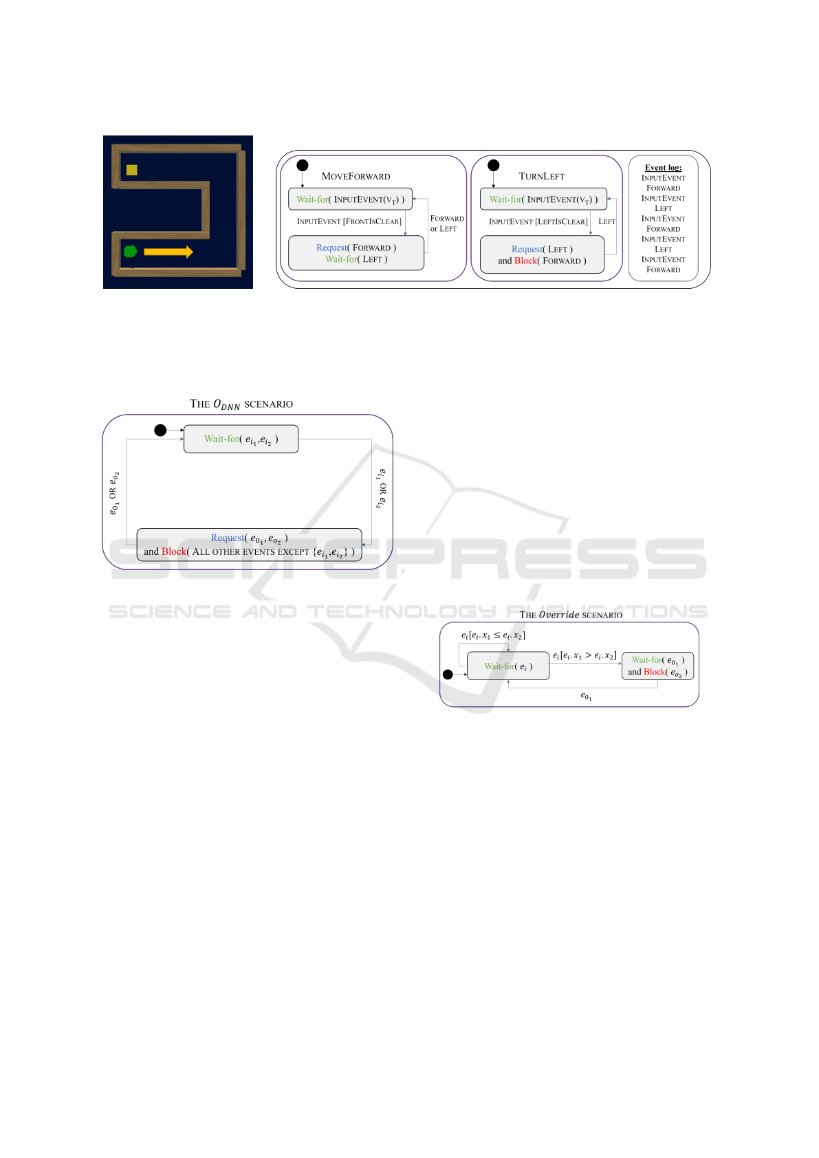
Figure 3: On the left, a screenshot of the Turtlebot simulator, where the robot is headed right and the target appears in the

top left corner. In the middle, the scenario-based model, written in Statechart-like transition systems (Harel, 1986) extended

with SBM. The model contains two scenarios: The MOVEFORWARD scenario and the TURNLEFT scenario. The black circles

specify the initial state. In each state the scenario can request, wait-for or block events. Once a requested/waited-for event

is triggered, the scenario transitions to the appropriate state (highlighted by a connecting edge with the event name and an

optional Boolean condition). On the right, a log of the triggered events during the execution, for this particular maze.

Figure 4: A ﬁgure of the O

DNN

scenario object correspond-

ing to the neural network in Fig. 1 described in statecharts.

The black circle indicates the initial state. The scenario

waits for the events e

and e

that represent the inputs to

the neural network. These events contain a payload with

the actual values assigned. The scenario then proceeds to

request the events e

and e

, which represent the possible

output labels y

, y

respectively (inspired by (Katz, 2021a)).

ride scenario can coerce the DNN to select a speciﬁc

output, by blocking all other output events; or it can

interfere in a more subtle manner, by blocking some

output events, while allowing O

DNN

to select from the

remaining ones. One strategy for selecting an alter-

nate output event in a classiﬁcation problem will be

to select the event with the next-to-highest score.

In practice, the requirement that the event sets I

and O be ﬁnite is restrictive, as DNNs typically have

a very large (effectively inﬁnite) number of possible

inputs. To overcome this restriction, we follow the ex-

tension proposed in (Katz et al., 2019), which enables

us to treat events as typed variables, or sets thereof.

Using this extension, the various scenarios can affect,

through requesting and blocking, the possible values

of these variables; and a scenario object’s transitions

may be conditioned upon the values of these vari-

ables. In particular, these variables can be used to

express an inﬁnite number of possible inputs and out-

puts of a DNN.

Using the aforementioned extension, the override

rule from Sec. 2.1 is depicted in Fig. 5. The scenario

waits for the input event e

, which now contains as

a payload two real-valued variables, x

and x

, that

represent the actual assignment to the DNN’s inputs.

The transitions of the scenario object are then condi-

tioned upon the values of these variables: if the pred-

icate P holds for this input, the scenario transitions to

its second state, where it overrides the DNN’s output

by blocking the output event e

, which necessarily

causes the triggering of e

Figure 5: A scenario object for enforcing the override rule

deﬁned in Sec. 2.2. The scenario waits for the input event e

and inspects the payload to see if the predicate P holds for

the given input. It then continues to wait for the output event

, while blocking the unwanted event e

. This blocking

forces the triggering of output event e

. Once this happens,

the scenario returns to its initial state.

3 CASE STUDY: THE AURORA

CONGESTION CONTROLLER

For our ﬁrst case study, we focus on Aurora (Jay et al.,

2019) — a recently proposed performance-oriented

congestion control (PCC) protocol, whose purpose is

to manage a computer network (e.g., the Internet).

Aurora’s goal is to maximize the network’s through-

put, and to prevent “congestive collapses”, i.e., sit-

Enhancing Deep Learning with Scenario-Based Override Rules: A Case Study

257

uations where the incoming trafﬁc rate exceeds the

outgoing bandwidth and packets are lost. Aurora is

to learn an optimal policy with respect to the envi-

ronment’s state and reward, which reﬂect the agent’s

performance in previous batches of sent packets. The

action selected by the agent is the sending rate that is

used for the next batch of packets. It has been shown

that Aurora can obtain impressive results, competitive

with modern, hand-crafted algorithms for similar pur-

poses (Jay et al., 2019).

Aurora employs the concept of monitor intervals

(MIs) (Dong et al., 2018), in which time is split into

consecutive intervals. At the start of each MI, the

agent’s chosen action a

(a real value) is selected as

the sending rate for the current MI, and it remains

ﬁxed throughout the interval. This rate affects the

pace, and eventually the throughput, of the protocol.

After the MI has ﬁnished, a vector v

containing real-

valued performance statistics is computed from data

collected during the interval. Subsequently, v

is pro-

vided as the environment state to the agent, which

then proceeds to select a new sending rate a

t+1

for

the next MI, and so on. For a more extensive back-

ground on performance-oriented congestion control,

see (Dong et al., 2015).

As a supporting tool, Aurora is distributed with

the PCC-DL simulator (Meng et al., 2020a) that en-

ables the user to test Aurora’s performance. The sim-

ulator has two built-in congestion control protocols:

• The PCC-IXP protocol: a simple protocol that ad-

justs the sending rate using a hard-coded function.

• The PCC-Python protocol: a protocol that utilizes

a trained Aurora agent to adjust the sending rate.

Both of these protocols are classiﬁed as normal (pri-

mary) protocols that aspire to maximize their through-

put (Meng et al., 2020b).

We chose Aurora as our ﬁrst case study because

of its reactive nature: it receives external input from

the environment, processes this information using

the trained DRL agent, and acts on it with the next

sending rate. SBM is well suited for reactive sys-

tems (Harel et al., 2012), and Aurora matched our

requirements to enhance a reactive DL system. The

goals we set out to achieve in this case study are de-

tailed in the following section.

3.1 Integrating Aurora and SBM

Our ﬁrst goal was to instrument the Aurora DNN

agent with the O

DNN

infrastructure, and integrate it

with an SB model. This was achieved through the

inclusion of the C++ SBM package (Harel and Katz,

2014; Katz, 2021b) in the simulator; and the intro-

duction of a new protocol, PCC-SBM, which extends

the PCC-Python protocol and launches an SB model

that includes the O

DNN

scenario. This process, on

which we elaborate next, required signiﬁcant techni-

cal work — and successfully produced an integrated

SBM/DNN model that performed on par with the

original, DNN-based model.

The simulator interacts with the PCC-SBM pro-

tocol in two ways: (i) it provides the statistics of the

current MI; and (ii) it requests the next sending rate.

Thus, we began the SBM/DNN integration by intro-

ducing a SENSOR scenario, whose purpose is to in-

ject MONITORINTERVAL and QUERYNEXTSENDIN-

GRATE events into the SB model, to allow it to com-

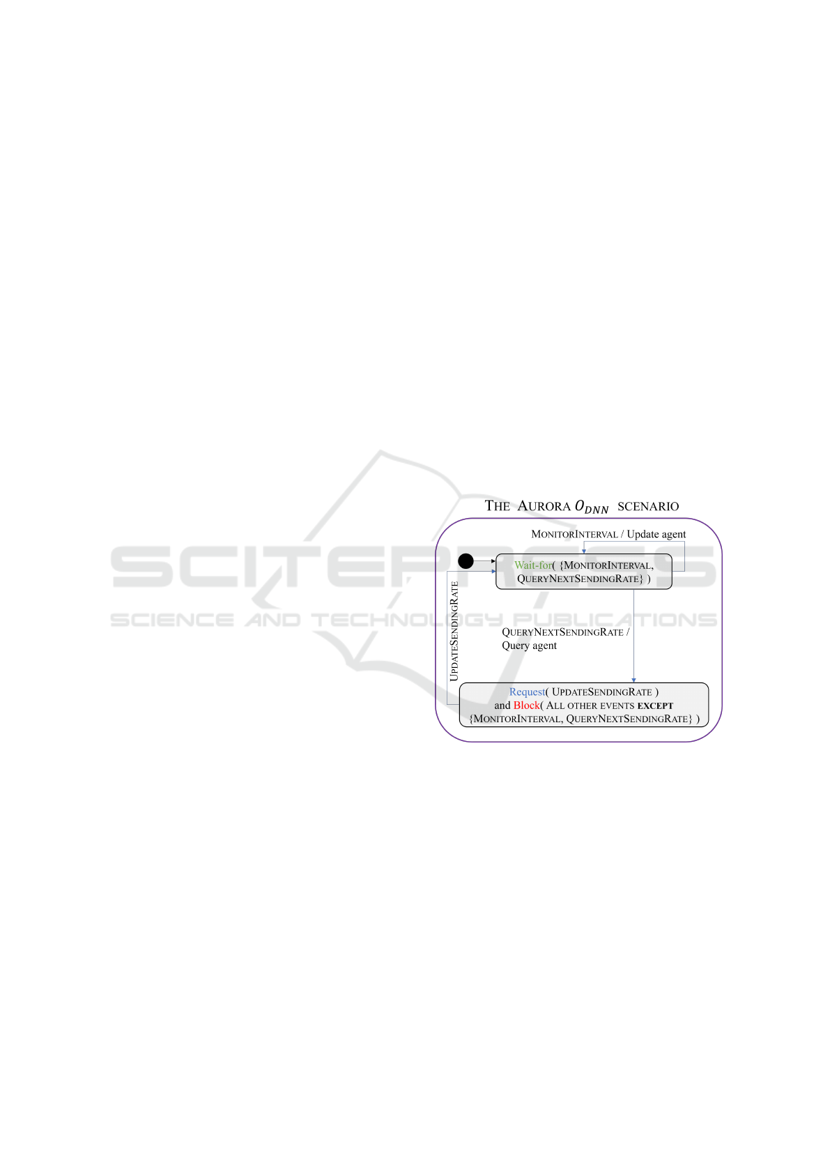
municate with the simulator. Fig. 6 depicts the AU-

RORA O

DNN

scenario (using a combination of State-

charts and SBM visual languages (Harel, 1986; Mar-

ron et al., 2018)), which waits for these events in its

initial state. The event MONITORINTERVAL carries,

as a payload, the MI statistics vector, v

, whose entries

are real values.

Figure 6: The AURORA O

DNN

scenario.

When MONITORINTERVAL is triggered, the

statistics vector is provided as the input to the under-

lying DNN, and when the event QUERYNEXTSEND-

INGRATE is triggered, the scenario extracts the

DNN’s output, and then uses it as a payload for

an UPDATESENDINGRATE that it requests — while

blocking all other, non-input events. Finally, we in-

troduce an ACTUATOR scenario, which waits for the

event UPDATESENDINGRATE and updates the simu-

lator on the selected sending rate for the next batch of

packets.

MODELSWARD 2023 - 11th International Conference on Model-Based Software and Systems Engineering

258

3.2 Supporting Scavenger Mode

For our second, more ambitious goal, we set out to

extend the Aurora system with a new behavior, with-

out altering its underlying DNN: speciﬁcally, with

the ability to support scavenger mode (Meng et al.,

2020b). The scavenger protocol is a “polite” protocol,

meaning it can yield its throughput if there is competi-

tion in the same physical network. Of course, such be-

havior needs to be temporary, and when the other traf-

ﬁc on the physical network subsides, the scavenger

protocol should again increase its throughput, utiliz-

ing as much of the available bandwidth as possible.

In order to add scavenger mode support, we added

the following scenarios:

• The MONITORNETWORKSTATE scenario object,

which inspects the state of the physical network

and requests a speciﬁc event: the ENTERYIELD

event that marks that the conditions for entering

yield mode, in which sending rates should be re-

duced, are met.

• The REDUCETHROUGHPUT scenario object,

which is an override scenario. This scenario ﬁrst

waits-for a notiﬁcation that the protocol should

enter yield mode, and then proceeds to override

the DNN’s calculated sending rate with a lower

sending rate.

Our plan was for the REDUCETHROUGHPUT scenario

to support three override policies: (i) an immediate

decline to a ﬁxed, low sending rate; (ii) a gradual de-

cline, using a step function; and (iii) a gradual de-

cline, using exponential decay. However, we quickly

observed that the existing override scenario formula-

tion (as presented in Sec. 2.4) was not suitable for this

task.

Recall that an override scenario overrides O

DNN

’s

output by blocking any unwanted output events, and

coercing the event selection mechanism to select a

different output event that is not blocked. In our case,

however, we needed REDUCETHROUGHPUT to act as

an override scenario that blocks some output events

based on the output selected by O

DNN

, in the current

time step. For example, in the case of a gradual de-

cline in the sending rate, if O

DNN

would normally se-

lect sending rate x, we might want to force the selec-

tion of rate

, instead; but this requires knowing the

value of x, in advance, which is simply not possible

using the current formulation (Katz, 2020).

To circumvent this issue within the existing mod-

eling framework, we introduce a new “proxy event”,

UPDATESENDINGRATEREDUCE, intended to serve

as a middleman between the AURORA O

DNN

sce-

nario and its consumers. Our override scenario, RE-

DUCETHROUGHPUT, no longer directly blocks cer-

tain values that the DNN might produce. Instead, it

waits-for the UPDATESENDINGRATE event produced

by AURORA O

DNN

, manipulates its real-valued pay-

load as needed, and then requests the proxy event

UPDATESENDINGRATEREDUCE with the (possibly)

modiﬁed value. Then, in every scenario that orig-

inally waited-for the UPDATESENDINGRATE event,

we rename the event to UPDATESENDINGRATERE-

DUCE, so that the scenario now waits for the proxy

event, instead. Fig. 7 visually illustrates the ﬁnal ver-

sion of the REDUCETHROUGHPUT scenario.

After entering scavenger mode and lowering the

sending rate, a natural requirement is that the sys-

tem eventually reverts to a higher sending rate, when

scavenger mode is no longer required. To achieve

this, we adjust the MONITORNETWORKSTATE sce-

nario to dynamically identify this situation, and sig-

nal to the other scenarios that the system has en-

tered restore mode, by requesting the event ENTER-

RESTORE. We then introduce a second override sce-

nario, RESTORETHROUGHPUT, that can increase the

protocol’s throughput according to one of two prede-

ﬁned policies: (i) an immediate return to the model’s

original output; or (ii) a slow start policy (Contribu-

tors, 2022a).

The RESTORETHROUGHPUT scenario waits-for

the events ENTERRESTORE, ENTERYIELD and UP-

DATESENDINGRATE. The ﬁrst two events signal the

scenario to enter/exit restore mode. When UPDATE-

SENDINGRATE is triggered and the scenario is in re-

store mode, it overrides the value according to the pol-

icy in use, and requests an output event with a modi-

ﬁed value. Utilizing the UPDATESENDINGRATERE-

DUCE event for this purpose would result in two,

likely contradictory output events being requested at a

single synchronization point. To avoid this, we intro-

duce a new event, UPDATESENDINGRATERESTORE,

to be requested by the RESTORETHROUGHPUT sce-

nario, while blocking the possible UPDATESENDIN-

GRATEREDUCE event at the synchronization point.

This decision prioritizes ratio restoration over yield-

ing (although any other prioritization rule could be

used). Finally, in every scenario that requests/waits-

for the UPDATESENDINGRATEREDUCE event, we

add a wait-for the UPDATESENDINGRATERESTORE

event. In this manner, these scenarios can proceed

with their execution despite being blocked.

3.3 Evaluation

For evaluation purposes, we implemented the sce-

nario objects described in Sec. 3.2, and then used Au-

rora’s simulator to evaluate the enhanced model’s per-

formance, compared to that of the original (Ashrov

Enhancing Deep Learning with Scenario-Based Override Rules: A Case Study

259

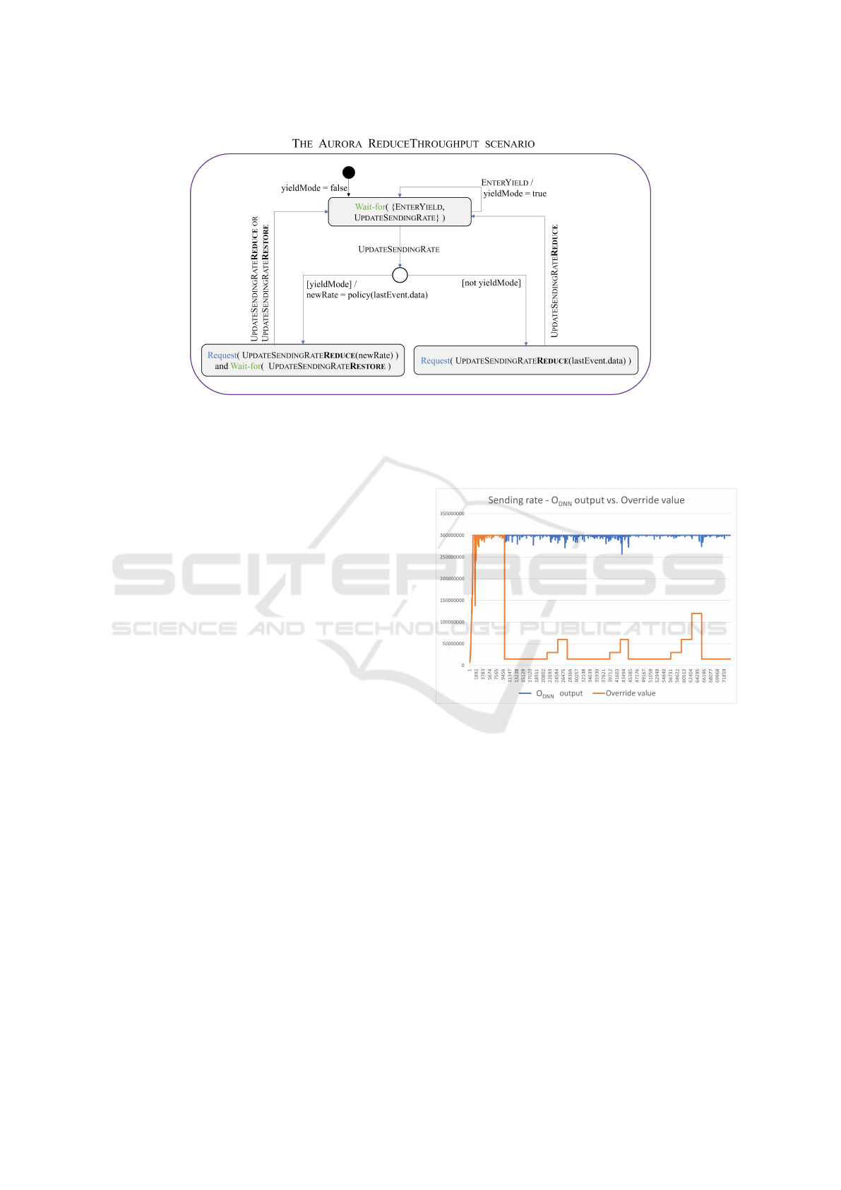
Figure 7: The Aurora REDUCETHROUGHPUT scenario, described using Statecharts enhanced with SBM. The black circle

speciﬁes the initial state. The scenario waits-for ENTERYIELD event to enter yield mode. If yield mode is enabled, the UP-

DATESENDINGRATE event payload will be modiﬁed, and the UPDATESENDINGRATEREDUCE will be requested. Otherwise,

the payload is propagated as-is in the “proxy” UPDATESENDINGRATEREDUCE event. The scenario waits for UPDATESEND-

INGRATERESTORE to return to its initial state, in case UPDATESENDINGRATEREDUCE is blocked.

and Katz, 2023). Our results, described below, in-

dicate that the modiﬁed system successfully supports

scavenger mode, although its internal DNN remained

unchanged.

Fig. 8 depicts the sending rate requested by the

AURORA O

DNN

scenario, following an input event

QUERYNEXTSENDINGRATE, and the actual sending

rate that was eventually returned to the simulator by

the PCC-SBM protocol. We notice that initially, the

two values coincide, indicating that no overriding is

triggered — because the MONITORNETWORKSTATE

scenario did not yet signal that the system should

enter yield mode. However, once this signal oc-

curs, the REDUCETHROUGHPUT scenario overrides

the sending rate, according to the ﬁxed rate policy.

After a while, the MONITORNETWORKSTATE de-

tects that it is time to once again increase the sending

rate, and signals that the system should enter restore

mode. As a result, we see an increase, per the “slow

start” restoration policy of RESTORETHROUGHPUT.

The ensuing back-and-forth switching between yield

and restore modes demonstrates that the MONITOR-

NETWORKSTATE scenario dynamically responds to

changes in environmental conditions.

In another experiment, we compared the through-

put (MB/s) of the primary PCC-IXP protocol with

that of the PCC-SBM protocol, when the two are ex-

ecuted in parallel. The results appear in Fig. 9. We

observe that there is a resemblance between the over-

ridden sending rate value seen in Fig. 8 and the actual

throughput. When the MONITORNETWORKSTATE

scenario signals to yield, the sending rate declines to a

ﬁxed value, which in turn leads to a ﬁxed throughput.

Figure 8: The AURORA O

DNN

original model output,

vs. the values produced by the override scenarios. The pol-

icy used for reduction is an immediate decline to a ﬁxed

rate. The policy used for restoration is “slow start”.

Additionally, when the sending rate increases after a

signal to restore, the throughput of the protocol in-

creases as well. Another interesting phenomenon is

that when the PCC-SBM relinquishes bandwidth, the

PCC-IXP increases its own throughput, which is the

behavior we expect to see. We speculate that the yield

of the PCC-SBM enabled this increase.

4 CASE STUDY: THE ROBOTIS

Turtlebot3 PLATFORM

For our second case study, we chose to enhance a DL

system trained by Corsi et al. (Corsi et al., 2022a;

MODELSWARD 2023 - 11th International Conference on Model-Based Software and Systems Engineering

260

Figure 9: The recorded throughput (MB/s) of the PCC-IXP

and PCC-SBM protocols, when executed in parallel using

the PCC simulator.

Corsi et al., 2022b), which aims to solve a setup of

the mapless navigation problem. The system con-

tains a DNN agent whose goal is to navigate a Turtle-

bot 3 (Turtlebot) robot (Robotis, 2023; Amsters and

Slaets, 2019) to a target destination, without collid-

ing with obstacles. Contrary to classical planning, the

robot does not hold a global map, but instead attempts

to navigate using readings from its environment. A

successful navigation policy must thus be dynamic,

adapting to changes in local observations as the robot

moves closer to its destination. DRL algorithms have

proven successful in learning such a policy (March-

esini and Farinelli, 2020).

We refer to the DNN agent that controls the Turtle-

bot as TRL (for Turtlebot using RL). The agent learns

a navigation policy iteratively: in each iteration, it

is provided with a vector v

that comprises (i) nor-

malized lidar scans of the robot’s distance from any

nearby obstacles; and (ii) the angle and the distance

of the robot from the target. The agent then evaluates

its internal DNN on v

, obtaining a vector v

that con-

tains a probability distribution over the set of possible

actions the Turtlebot can perform: moving forward, or

turning left or right. For example, one possible vec-

tor is v

= [(Forward,0.2), (Left, 0.5), (Right, 0.3)].

Using this vector, the agent then randomly selects

an action according to the distribution, navigates the

Turtlebot, and receives a reward.

The DNN at the core of the TRL controller is

trained and tested in a simulation environment that

contains a sim-robot Turtlebot 3 burger (Robotis,

2023), and a single, ﬁxed maze, created using the

ROS2 framework (ROS, 2023) and the Unity3D en-

gine (Unity, 2023). In each session, the robot’s start-

ing location is drawn randomly, which enables a di-

verse scan of the input space. The navigation session

has four possible outcomes: (i) success; (ii) collision;

(iii) timeout; or (iv) an unknown failure.

We selected the Turtlebot project as our second

case study due to its reactive characteristics: it reads

external information using its sensors, applies an in-

ternal logic to select the next action, and then acts

by moving towards the target. SBM has previously

been applied to model robot navigation and maze

solving (Elyasaf, 2021; Ashrov et al., 2017), which

strengthened our intuition that an enhancement of the

Turtlebot with SBM is feasible. Next, we outline the

objectives we aimed to achieve in this case study.

4.1 Integrating Turtlebot and SBM

Similarly to the Aurora case, our ﬁrst goal was to in-

strument the Turtlebot DNN with the O

DNN

infras-

tructure, so that it could be composed with an SB

model. This was achieved by using the Python im-

plementation of SBM (Yaacov, 2020), and integrating

it with the TRL code. We created a SENSOR scenario

that waits for the current state vector v

, and injects an

INPUTEVENT containing v

into the SB model; and

also an ACTUATOR scenario that waits for an internal

OUTPUTEVENT, and transmits its action as the one to

be carried out by the Turtlebot.

Next, we proceeded to create the TURTLEBOT

DNN

scenario for TRL. Unlike in the Aurora case,

where the DNN would output a single chosen event,

here the DNN outputs a probability distribution over

the possible actions (a common theme in DRL-based

systems (Sutton and Barto, 2018)). To accommo-

date this, we adjusted our O

DNN

scenario to request

all the possible output events in the form of a vec-

tor P

, which contains each possible action and its

probability. We then modiﬁed SBM’s event selec-

tion mechanism to randomly select a requested out-

put event from P

, with respect to the induced prob-

ability distribution. The mechanism then triggers the

OUTPUTEVENT, which contains in its payload the se-

lected action and its probability. During modeling and

experimentation, the scenario can assign any proba-

bility distribution (e.g., uniform) to the DNN’s output

events; and during deployment, these values are com-

puted using the actual DNN (see Fig. 10). If the event

selection mechanism selects an event that is blocked,

the selection is repeated, until a non-blocked event is

selected. If there are no enabled events, then the sys-

tem is deadlocked and the program ends. Using this

approach, our Turtlebot controller could successfully

navigate in various mazes.

Once the O

DNN

infrastructure was in place, we

veriﬁed that the augmented program’s performance

was similar to that of the original agent. This

was achieved by comparing the models pre-trained

Enhancing Deep Learning with Scenario-Based Override Rules: A Case Study

261

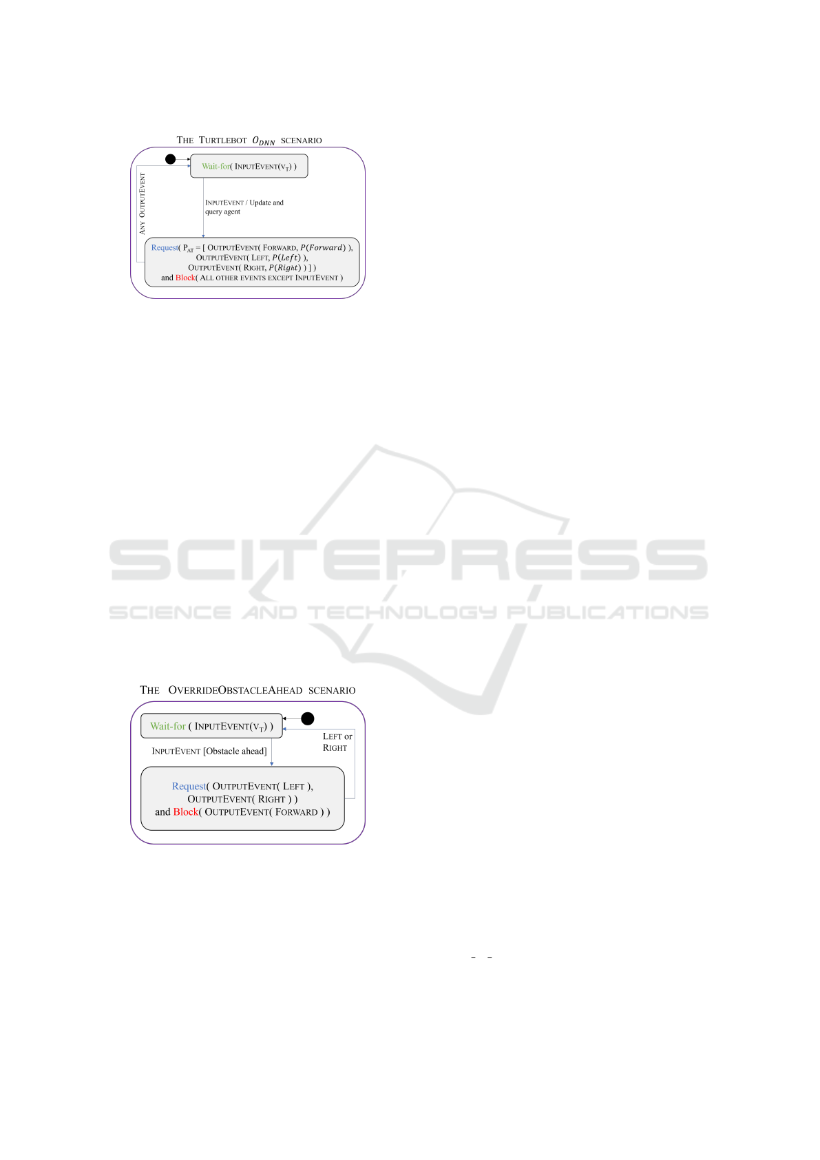
Figure 10: The TURTLEBOT O

DNN

scenario. The scenario

waits for an INPUTEVENT containing v

, provides it to the

agent, and receives a vector P

of possible actions and prob-

abilities. It then proceeds to request all the output events

from the ESM using P

. At the synchronization point, the

ESM executes the TURTLEBOT O

DNN

event selection strat-

egy, and one possible OUTPUTEVENT is triggered.

by (Corsi et al., 2022a) to our SBM-enhanced ver-

sion, and checking that both agents obtained similar

success rates on various mazes.

4.2 A Conservative Controller

For our second goal, we sought to increase the

model’s safety, by implementing a basic override rule,

OVERRIDEOBSTACLEAHEAD, which would prevent

the Turtlebot from colliding with an obstacle that is

directly ahead. This can be achieved by analyzing the

DNN’s inputs, which include the lidar readings, and

identifying cases where a move forward would guar-

antee a collision; and then blocking this move, forcing

the system to select a different action. An illustration

of this simple override rule appears in Fig. 11.

Figure 11: The OVERRIDEOBSTACLEAHEAD scenario

waits for an INPUTEVENT containing v

, and inspects the

lidar sensors facing forward readings. If distance < 0.22,

moving forward will cause a collision. Therefore the sce-

nario blocks the OUTPUTEVENT(FORWARD) event.

As we were experimenting with the Turtlebot

and various override rules, we noticed the follow-

ing, interesting pattern. Recall that a Turtlebot agent

learns a policy, which, for a given state s

, pro-

duces a probability distribution over the actions, a

[P(Forward), P(Left), P(Right)]. We can regard this

vector as the agent’s conﬁdence levels that each of the

possible actions will bring the Turtlebot closer to its

goal. The random selection that follows takes these

conﬁdence levels into account, and is more likely to

select an action that the agent is conﬁdent about; but

this is not always the case. Speciﬁcally, we observed

that for “weaker” models, e.g. models with about a

50% success rate, the agent would repeatedly select

actions with a low conﬁdence score, which would of-

ten lead to a collision. This observation led us to de-

sign our next override scenario, CONSERVATIVEAC-

TION, which is intended to force the agent to select

actions only when their conﬁdence score meets a cer-

tain threshold.

Ideally, we wish for CONSERVATIVEACTION to

implement the following behavior: (i) wait-for the

OUTPUTEVENT being selected (ii) examine whether

the conﬁdence score in its payload is below a certain

threshold, and if so, (iii) apply blocking to ensure that

a different OUTPUTEVENT, with a higher score, is se-

lected for triggering. This method again requires that

the override scenario be able to inspect the content

of the OUTPUTEVENT being triggered in the current

time step.

To overcome this issue, we add a new, proxy event

called OUTPUTEVENTPROXY, and adjust all exist-

ing scenarios that would previously wait for OUT-

PUTEVENT to wait for this new event, instead. Then,

we have the CONSERVATIVEACTION scenario wait-

for the input event to O

DNN

, and have it replay

that event to initiate additional evaluations of the

DNN, and the ensuing random picking of the OUT-

PUTEVENT, until an acceptable output action is se-

lected. When this occurs, the CONSERVATIVEAC-

TION scenario propagates the selected action as an

OUTPUTEVENTPROXY event.

4.3 Evaluation

For evaluation purposes, we trained a collection

of agents, C

agents

, using the technique of Corsi et

al. (Corsi et al., 2022b). These agents had varying

success rates, ranging from 4% to 96%. Next, we

compared the performance of these agents to their

performance when enhanced by our SB model.

In the ﬁrst experiment, we disabled our override

rule, and had every agent in C

agents

solve a maze from

100 different random starting points. The statistics we

measured were:

• num of solved: the number of times the agent

reached the target.

MODELSWARD 2023 - 11th International Conference on Model-Based Software and Systems Engineering

262

• num of collision: the number of times the agent

collided with an obstacle.

• avg num of steps: the average number of steps

the agent performed in a successful navigation.

We then repeated this setting with the CONSERVA-

TIVEACTION scenario enabled.

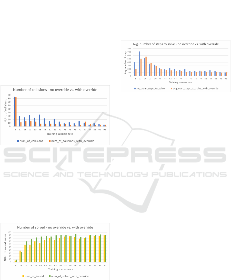
The experiment’s results are summarized in

Fig. 12, and show that enabling the override rule

leads to a signiﬁcant reduction in the number of col-

lisions. We notice that, as the agent’s success rate in-

creases, the improvement rate decreases. One hypoth-

esis for this behavior could be that “stronger” mod-

els are more conﬁdent in their recommended actions,

thus requiring fewer activations of the override rule.

Figure 12: Comparing the number of collisions when the

CONSERVATIVEACTION override is disabled and then en-

abled.

Fig. 13 portrays a general improvement in the

agent’s success rate when the override rule is enabled,

which is (unsurprisingly) correlated with the reduc-

tion in the number of collisions. A possible expla-

nation is that “mediocre” agents, i.e. those with suc-

cess rates in the range between 16% and 70%, learned

policies that are good enough to navigate towards the

target, but which require some assistance in order to

avoid obstacles along the way.

Figure 13: Comparing the num. of solved mazes when the

CONSERVATIVEACTION override is disabled and then en-

abled.

Fig. 14 depicts a reduction in the average num-

ber of steps required for an agent to solve the maze,

when the override scenario is enabled. This somewhat

surprising result indicates that although our agents

can successfully solve mazes, the CONSERVATIVE-

ACTION scenario renders their navigation more efﬁ-

cient. We speculate that for these agents, selecting

actions with low conﬁdence scores leads to redundant

steps.

Figure 14: Comparing the average number of steps to solve

when the CONSERVATIVEACTION override is disabled and

then enabled.

5 INTRODUCING MODIFIER

SCENARIOS

5.1 Motivation

In both of our case studies, we needed to create sce-

narios capable of reasoning about the events being re-

quested in the current time step — which we resolved

by introducing new, “proxy” events. However, such

a solution has several drawbacks. First, it entails ex-

tensive renaming of existing events, and the modiﬁ-

cation of existing scenarios, which goes against the

incremental nature of SBM (Harel et al., 2012). Sec-

ond, once added, the override scenario becomes a cru-

cial component in the O

DNN

infrastructure, without

which the system cannot operate; and in the common

case where the override rule is not triggered, this in-

curs unnecessary overhead. Third, it is unclear how to

support the case where several scenarios are required.

These drawbacks indicate that the “proxy” solution is

complex, costly, and leaves much to be desired.

In order to address this need and allow users to de-

sign override rules in a more convenient manner, we

propose here to extend the idioms of SBM in a way

that will support modiﬁer scenarios: scenarios that

are capable of observing and modifying the current

event, as it is being selected for triggering. A formal

deﬁnition appears below.

Enhancing Deep Learning with Scenario-Based Override Rules: A Case Study

263

5.2 Deﬁning Modiﬁer Scenarios

We extend the deﬁnitions of SBM from Sec. 2 with

a new type of scenario, named a modiﬁer scenario.

A modiﬁer scenario is formally deﬁned as a tuple

modiﬁer

= ⟨Q

, q

, δ

, f

⟩, where:

• Q

is a set of states representing synchronization

points.

• q

is the initial state.

• δ

: Q

× E → Q

is a deterministic transition

function, indicating how the scenario reacts when

an event is triggered.

• f

: Q

× 2

→ E is a function that maps

a state, a set of observed requested events, and a

set of observed blocked events into an event from

the set E. f

can operate in a deterministic, well-

deﬁned manner, or in a randomized manner to se-

lect a suitable event from E.

Intuitively, the modiﬁer thread can use its function f

at a synchronization point to affect the selection of the

current event.

Let M = {O

, ...,O

, O

modiﬁer

} be a behavioral

model, where n ∈ N, each O

= ⟨Q

, q

, δ

, R

, B

⟩ is

an ordinary scenario object, and O

modiﬁer

is a mod-

iﬁer scenario object. In order to deﬁne the seman-

tics of M, we construct the labeled transition system

LTS(M) = ⟨Q, q

, δ, f

⟩, where:

• Q := Q

× ... × Q

× Q

is the set of states.

• q

:= ⟨q

, ...,q

, q

⟩ ∈ Q is the initial state.

• f

:= f

is the modiﬁcation function of O

modiﬁer

• δ : Q × E → Q is a deterministic transition func-

tion, deﬁned for all q = ⟨q

, ...,q

, q

⟩ ∈ Q and

e ∈ E by

δ(q, e) := ⟨δ

, e), ..., δ

, e), δ

, e)⟩

An execution of P is an execution of LTS(M).

The execution starts from the initial state q

, and in

each state q ∈ Q, the event selection mechanism col-

lects the sets of requested and blocked events, namely

R(q) :=

i=1

) and B(q) :=

i=1

The set of enabled events at synchronization point

q is E(q) = R(q)\B(q). If E(q) =

0 then the system is

deadlocked. Otherwise, the ESM allows the modiﬁer

scenario to affect event selection, by applying f

and

selecting the event:

e = f

(q, R(q),B(q)).

The ESM then triggers e, and notiﬁes the relevant

scenarios. By convention, we require that f

does

not select an event that is currently blocked; although

it can select events that are not currently requested.

The state of LTS(M) is then updated according to e.

The execution of LT S(M) is formally recorded as a

sequence of triggered events (a run). For simplicity,

we assume that there is a single O

modiﬁer

object in the

model, although in practice it can be implemented us-

ing a collection of scenarios.

5.3 Revised Override Scenarios

We extend the deﬁnition of an override rule over a

network N, into a tuple ⟨P, Q, f ⟩, where: (i) P(x)

is a predicate over the network’s input vector x;

(ii) Q(N(x)) is a predicate over the network’s output

vector N(x); and (iii) f : O → O is a function that re-

places the proposed network output event with a new

output event. Using a modiﬁer scenario O

modiﬁer

, we

can now implement this more general form of an over-

ride rule within an SB model. As an illustrative ex-

ample, we change the override rule from Sec. 2.2, to

consider the network’s output as well:

⟨x

> x

, y

> 1, f (y

) → y

⟩

Note that this deﬁnition differs from the origi-

nal: it takes into account the currently selected out-

put event and its value. Also, it contains a function f

that, whenever the predicates hold, maps a network-

selected output into action y

. An updated version of

the override rule, implemented as a modiﬁer scenario,

appears in Fig. 15. To support the ability to observe

output event e

’s internal value, the event contains a

payload of the calculated output neurons’ values.

Figure 15: An O

modiﬁer

scenario object for enforcing the

override rule that whenever x

> x

and y

> 1, output event

should be triggered. The scenario waits for the input

event to satisfy the predicate, and then proceeds to the state

where it declares a modiﬁcation. The ﬁrst argument to the

modiﬁcation function f is the output event and assignment

that the scenario would like to modify. The second argu-

ment to the function is the set of blocked events: None, in

our case. The return value from the function is the output

event, e

. At the synchronization point, the ESM collects

the requested and blocked events, applies the f function of

the modiﬁer scenario, and then notiﬁes the relevant scenar-

ios that e

output event has been selected for triggering.

With the updated override rule deﬁnition, we now

refactor the scenarios from Sec. 3.2. First, we re-

store UPDATESENDINGRATE to its original role as

MODELSWARD 2023 - 11th International Conference on Model-Based Software and Systems Engineering

264

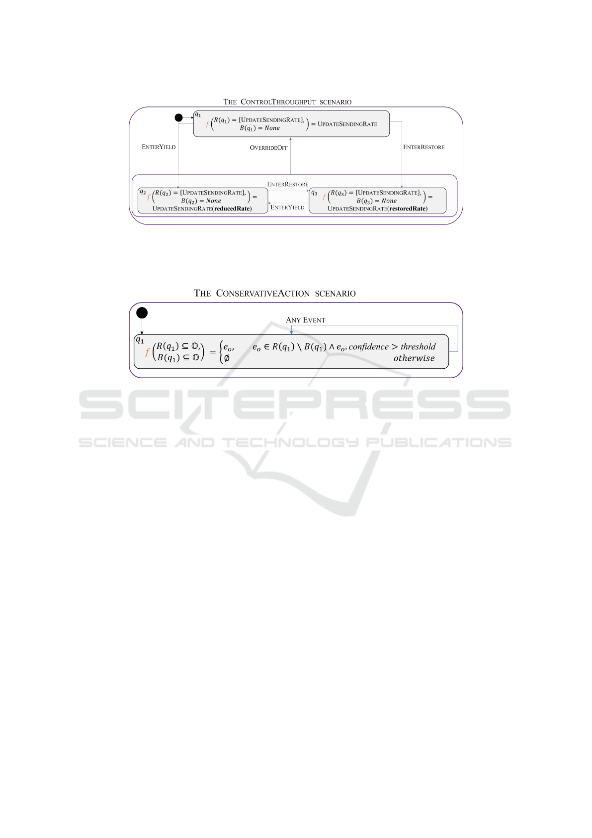
Figure 16: The CONTROLTHROUGHPUT override scenario. The scenario waits-for events

{OVERRIDEOFF,ENTERYIELD,ENTERRESTORE} in each state, and transitions subsequently. It also observes and

possibly modiﬁes the UPDATESENDINGRATE event using its f function depending on the current state q

, R(q

) and B(q

E.g., if we are in q

, and UPDATESENDINGRATE is requested but not blocked, its value will be modiﬁed according to the

reduce policy. Note that the modiﬁcation of the UPDATESENDINGRATE does not result in a transition to a different state.

Figure 17: The revised CONSERVATIVEACTION scenario. The scenario observes all possible subsets of the output events O

that are requested or blocked at state q

. Concretely, at each synchronization point, the ESM launches f with a speciﬁc set of

the requested and blocked output events. The function f is only concerned with the set of enabled (requested and not blocked)

output events. From these possible output events, f randomly selects an event e

according to this policy: (i) if the selected

event is above the threshold, f passes the event as-is; and (ii) if the selected event is below the threshold, f randomly selects

a different possible output event which is above the threshold. The ESM then notiﬁes the relevant scenarios of the selected

output event. If no such event exists, the program is in a deadlock, in which case the scenario can reduce the threshold to ﬁnd

a possible event. The scenario remains in its state q

whenever any event is triggered.

an output event (as opposed to a proxy event). Sec-

ond, we modify the MONITORNETWORKSTATE sce-

nario to request three events that signal the cur-

rent throughput state: (i) OVERRIDEOFF, which sig-

nals that the sending rate should be forwarded as-

is; and (ii) ENTERYIELD and (iii) ENTERRESTORE,

which signal that the sending rate should be over-

ridden by the yield/restore policy. Third, we in-

troduce the CONTROLTHROUGHPUT override sce-

nario, replacing REDUCETHROUGHPUT and RE-

STORETHROUGHPUT. This scenario waits-for a sig-

nal on the current throughput state, and transitions be-

tween the internal states that represent it. The sce-

nario uses function f to observe the requested event

UPDATESENDINGRATE in each state. When the

output event UPDATESENDINGRATE is requested, f

is executed and receives the requested and blocked

events as parameters. If the event is blocked, we are

in a deadlock. If the scenario is in the OVERRIDEOFF

state, the function returns the event as-is. If the sce-

nario is in the ENTERYIELD/ ENTERRESTORE states,

the scenario returns an UPDATESENDINGRATE event

with a sending rate that is modiﬁed according to

the matching policy. The revised UPDATESENDIN-

GRATE event is then triggered, and all relevant sce-

narios proceed with their execution. Fig. 16 depicts

the new CONTROLTHROUGHPUT scenario.

We now revise the set of scenarios we imple-

mented to support the TRL project 4 and the conser-

vative override rule 4.2. The ﬁrst modiﬁcation is to

restore the OUTPUTEVENT event to its original role

as an output, instead of a proxy event. We then use the

f function to simplify the CONSERVATIVEACTION

scenario. Recall that originally, the scenario waited

for the INPUTEVENT, for the purpose of re-playing

the O

DNN

evaluation if the selected OUTPUTEVENT

was below the threshold. The revised scenario can

deﬁne an f that will observe the set of requested out-

put events, and then randomly select an output event

that exceeds the threshold, and which is not blocked.

If there are no possible output events, the system is

deadlocked. From a practical point of view, the sce-

Enhancing Deep Learning with Scenario-Based Override Rules: A Case Study

265

nario can reduce the threshold to avoid this situation

(assuming that R(q) \ B(q) is not empty). Fig. 17 dis-

plays the revised CONSERVATIVEACTION scenario.

In summary, we have successfully revised the

override rules from our two case studies utilizing the

modiﬁer

extension. First, this new and more power-

ful deﬁnition has enabled us to implement the rules

without “proxy” events. This change reduces the high

coupling between the scenarios of the original im-

plementation. Second, the redesigned models offer

a more compact and direct approach: (i) the two over-

ride rules from the Aurora case study were reduced

to a single scenario; and (ii) the TRL override rule

contains a single synchronization point. These char-

acteristics are more in line with the SBM spirit that

views scenarios as simple and self-contained compo-

nents. Moving forward, we plan to enhance the exist-

ing SBM packages with the O

modiﬁer

extension.

6 RELATED WORK

Override rules are becoming an integral part of many

DRL-based systems (Katz, 2020). The concept is

closely related to that of shields and runtime moni-

tors, which have been extensively used in the ﬁeld

of robotics (Phan et al., 2017), drones (Desai et al.,

2018), and many others (Hamlen et al., 2006; Falcone

et al., 2011; Schierman et al., 2015; Ji and Lafortune,

2017; Wu et al., 2018). We regard our work as an-

other step towards the goal of effectively creating, and

maintaining, override rules for complex systems.

Although our focus here has been on designing

override rules using SBM, other modeling formalisms

could be used just as well. Notable examples in-

clude the publish-subscribe framework (Eugster et al.,

2003), aspect oriented programming (Kiczales et al.,

1997), and the BIP formalism (Bliudze and Sifakis,

2008). A key property of SBM, which seems to ren-

der it a good ﬁt for override rules, is the native idiom

support for blocking events (Katz, 2020); although

similar support could be obtained, using various con-

structs, in other formalisms.

7 CONCLUSION

As DNNs are increasingly being integrated into com-

plex systems, there is a need to maintain, extend and

adjust them — which has given rise to the creation

of override rules. In this work, we sought to con-

tribute to the ongoing effort of facilitating the creation

of such rules, through two extensive case studies. Our

efforts exposed a difﬁculty in an existing, SBM-based

method for designing guard rules, which we were then

able to mitigate by extending the SBM framework it-

self. We hope that this effort, and others, will give rise

to formalisms that are highly equipped for supporting

engineers in designing override rules for DNN-based

systems.

ACKNOWLEDGEMENTS

We thank the anonymous reviewers for their insight-

ful comments. This work was partially supported

by the Israeli Smart Transportation Research Center

(ISTRC).

REFERENCES

Amsters, R. and Slaets, P. (2019). Turtlebot 3 as a Robotics

Education Platform. In Proc. 10th Int. Conf. on

Robotics in Education (RiE), pages 170–181.

Ashrov, A., Gordon, M., Marron, A., Sturm, A., and

Weiss, G. (2017). Structured Behavioral Program-

ming Idioms. In Proc. 18th Int. Conf. on Enterprise,

Business-Process and Information Systems Modeling

(BPMDS), pages 319–333.

Ashrov, A. and Katz, G. (2023). Enhancing Deep

Learning with Scenario-Based Override Rules

— Code Base. https://github.com/adielashrov/

Enhance-DL-with-SBM-Modelsward2023.

Ashrov, A., Marron, A., Weiss, G., and Wiener, G. (2015).

A Use-Case for Behavioral Programming: an Archi-

tecture in JavaScript and Blockly for Interactive Ap-

plications with Cross-Cutting Scenarios. Science of

Computer Programming, 98:268–292.

Avni, G., Bloem, R., Chatterjee, K., Henzinger, T.,

Konighofer, B., and Pranger, S. (2019). Run-Time

Optimization for Learned Controllers through Quan-

titative Games. In Proc. 31st Int. Conf. on Computer

Aided Veriﬁcation (CAV), pages 630–649.

Bar-Sinai, M., Weiss, G., and Shmuel, R. (2018a). BPjs—

a Framework for Modeling Reactive Systems using a

Scripting Language and BP. Technical Report. http:

//arxiv.org/abs/1806.00842.

Bar-Sinai, M., Weiss, G., and Shmuel, R. (2018b). BPjs:

an Extensible, Open Infrastructure for Behavioral Pro-

gramming Research. In Proc. 21st ACM/IEEE Int.

Conf. on Model Driven Engineering Languages and

Systems (MODELS), pages 59–60.

Bliudze, S. and Sifakis, J. (2008). A Notion of Glue Ex-

pressiveness for Component-Based Systems. In Proc.

19th Int. Conf. on Concurrency Theory (CONCUR),

pages 508–522.

Bojarski, M., Del Testa, D., Dworakowski, D., Firner, B.,

Flepp, B., Goyal, P., Jackel, L., Monfort, M., Muller,

U., Zhang, J., Zhang, X., Zhao, J., and Zieba, K.

(2016). End to End Learning for Self-Driving Cars.

Technical Report. http://arxiv.org/abs/1604.07316.

MODELSWARD 2023 - 11th International Conference on Model-Based Software and Systems Engineering

266

Collobert, R., Weston, J., Bottou, L., Karlen, M.,

Kavukcuoglu, K., and Kuksa, P. (2011). Natural Lan-

guage Processing (almost) from Scratch. Journal of

Machine Learning Research, 12:2493–2537.

Contributors, W. (2022a). TCP Slow start — Wikipedia,

The Free Encyclopedia. https://en.wikipedia.org/wiki/

TCP congestion control#Slow start.

Contributors, W. (2022b). Wall follower — Maze-

solving algorithm — Wikipedia, The Free Encyclo-

pedia. https://en.wikipedia.org/wiki/Maze-solving

algorithm#Wall follower.

Corsi, D., Yerushalmi, R., Amir, G., Farinelli, A., Harel,

D., and Katz, G. (2022a). Constrained Reinforcement

Learning for Robotics via Scenario-Based Program-

ming. Technical Report. https://arxiv.org/abs/2206.

09603.

Corsi, D., Yerushalmi, R., Amir, G., Farinelli, A., Harel,

D., and Katz, G. (2022b). Constrained Reinforce-

ment Learning for Robotics via Scenario-Based Pro-

gramming — Code Base. https://github.com/d-corsi/

ScenarioBasedRL.

Desai, A., Ghosh, S., Seshia, S. A., Shankar, N., and Tiwari,

A. (2018). Soter: Programming Safe Robotics System

using Runtime Assurance. Technical Report. http://

arxiv.org/abs/1808.07921.

Dong, M., Li, Q., Zarchy, D., Godfrey, P. B., and Schapira,

M. (2015). {PCC}: Re-Architecting Congestion Con-

trol for Consistent High Performance. In Proc. 12th

USENIX Symposium on Networked Systems Design

and Implementation (NSDI), pages 395–408.

Dong, M., Meng, T., Zarchy, D., Arslan, E., Gilad, Y.,

Godfrey, B., and Schapira, M. (2018). PCC Vivace:

Online-Learning Congestion Control. In Proc. 15th

USENIX Symposium on Networked Systems Design

and Implementation (NSDI), pages 343–356.

Elyasaf, A. (2021). Context-Oriented Behavioral Pro-

gramming. Information and Software Technology,

133:106504.

Eugster, P., Felber, P., Guerraoui, R., and Kermarrec, A.-M.

(2003). The Many Faces of Publish/Subscribe. ACM

Computing Surveys (CSUR), 35(2):114–131.

Falcone, Y., Mounier, L., Fernandez, J., and Richier, J.

(2011). Runtime Enforcement Monitors: Compo-

sition, Synthesis, and Enforcement Abilities. Jour-

nal on Formal Methods in System Design (FMSD),

38(3):223–262.

Goodfellow, I., Bengio, Y., and Courville, A. (2016). Deep

learning. MIT press.

Gordon, M., Marron, A., and Meerbaum-Salant, O. (2012).

Spaghetti for the Main Course? Observations on

the Naturalness of Scenario-Based Programming. In

Proc. 17th Conf. on Innovation and Technology in

Computer Science Education (ITICSE), pages 198–

203.

Hamlen, K., Morrisett, G., and Schneider, F. (2006).

Computability Classes for Enforcement Mechanisms.

ACM Transactions on Programming Languages and

Systems (TOPLAS), 28(1):175–205.

Harel, D. (1986). A Visual Formalism for Complex Sys-

tems. Science of Computer Programming, 8(3).

Harel, D., Kantor, A., and Katz, G. (2013). Relaxing Syn-

chronization Constraints in Behavioral Programs. In

Proc. 19th Int. Conf. on Logic for Programming, Arti-

ﬁcial Intelligence and Reasoning (LPAR), pages 355–

372.

Harel, D. and Katz, G. (2014). Scaling-Up Behavioral Pro-

gramming: Steps from Basic Principles to Applica-

tion Architectures. In Proc. 4th SPLASH Workshop

on Programming based on Actors, Agents and Decen-

tralized Control (AGERE!), pages 95–108.

Harel, D., Katz, G., Lampert, R., Marron, A., and Weiss, G.

(2015a). On the Succinctness of Idioms for Concur-

rent Programming. In Proc. 26th Int. Conf. on Con-

currency Theory (CONCUR), pages 85–99.

Harel, D., Katz, G., Marelly, R., and Marron, A. (2016).

An Initial Wise Development Environment for Behav-

ioral Models. In Proc. 4th Int. Conf. on Model-Driven

Engineering and Software Development (MODEL-

SWARD), pages 600–612.

Harel, D., Katz, G., Marelly, R., and Marron, A. (2018).

Wise Computing: Toward Endowing System Devel-

opment with Proactive Wisdom. IEEE Computer,

51(2):14–26.

Harel, D., Katz, G., Marron, A., and Weiss, G. (2014). Non-

Intrusive Repair of Safety and Liveness Violations in

Reactive Programs. Transactions on Computational

Collective Intelligence (TCCI), 16:1–33.

Harel, D., Katz, G., Marron, A., and Weiss, G. (2015b). The

Effect of Concurrent Programming Idioms on Veri-

ﬁcation. In Proc. 3rd Int. Conf. on Model-Driven

Engineering and Software Development (MODEL-

SWARD), pages 363–369.

Harel, D., Marron, A., and Sifakis, J. (2022). Creating

a Foundation for Next-Generation Autonomous Sys-

tems. IEEE Design & Test.

Harel, D., Marron, A., and Weiss, G. (2010). Programming

Coordinated Behavior in Java. In Proc. European

Conf. on Object-Oriented Programming (ECOOP),

pages 250–274.

Harel, D., Marron, A., and Weiss, G. (2012). Behav-

ioral programming. Communications of the ACM,

55(7):90–100.

Jay, N., Rotman, N., Godfrey, B., Schapira, M., and Tamar,

A. (2019). A Deep Reinforcement Learning Per-

spective on Internet Congestion Control. In Proc.

Int. Conf. on Machine Learning (ICML), pages 3050–

3059.

Ji, Y. and Lafortune, S. (2017). Enforcing Opacity by Pub-

licly Known Edit Functions. In Proc. 56th IEEE An-

nual Conf. on Decision and Control (CDC), pages 12–

15.

Julian, K., Lopez, J., Brush, J., Owen, M., and Kochender-

fer, M. (2016). Policy Compression for Aircraft Col-

lision Avoidance Systems. In Proc. IEEE/AIAA 35th

Digital Avionics Systems Conference (DASC), pages

1–10.

Jumper, J., Evans, R., Pritzel, A., Green, T., Figurnov,

M., Ronneberger, O., Tunyasuvunakool, K., Bates, R.,

ıdek, A., Potapenko, A., et al. (2021). Highly Accu-

Enhancing Deep Learning with Scenario-Based Override Rules: A Case Study

267

rate Protein Structure Prediction with Alphafold. Na-

ture, 596(7873):583–589.

Katz, G. (2013). On Module-Based Abstraction and Re-

pair of Behavioral Programs. In Proc. 19th Int. Conf.

on Logic for Programming, Artiﬁcial Intelligence and

Reasoning (LPAR), pages 518–535.

Katz, G. (2020). Guarded Deep Learning using Scenario-

Based Modeling. In Proc. 8th Int. Conf. on

Model-Driven Engineering and Software Develop-

ment (MODELSWARD), pages 126–136.

Katz, G. (2021a). Augmenting Deep Neural Networks

with Scenario-Based Guard Rules. Communica-

tions in Computer and Information Science (CCIS),

1361:147–172.

Katz, G. (2021b). Behavioral Programming in C++. https:

//github.com/adielashrov/bpc.

Katz, G., Marron, A., Sadon, A., and Weiss, G. (2019).

On-the-Fly Construction of Composite Events in

Scenario-Based Modeling Using Constraint Solvers.

In Proc. 7th Int. Conf. on Model-Driven Engineering

and Software Development (MODELSWARD), pages

143–156.

Kiczales, G., Lamping, J., Mendhekar, A., Maeda, C.,

Lopes, C., Loingtier, J.-M., and Irwin, J. (1997).

Aspect-Oriented Programming. In Proc. European

Conf. on Object-Oriented Programming (ECOOP),

pages 220–242.

Marchesini, E. and Farinelli, A. (2020). Discrete Deep

Reinforcement Learning for Mapless Navigation. In

Proc. IEEE Int. Conf. on Robotics and Automation

(ICRA), pages 10688–10694.

Marron, A., Hacohen, Y., Harel, D., M

ulder, A., and Ter-

ﬂoth, A. (2018). Embedding Scenario-based Model-

ing in Statecharts. In Proc. 21st ACM/IEEE Int. Conf.

on Model Driven Engineering Languages and Systems

(MODELS), pages 443–452.

Meng, T., Jay, N., and Godfrey, B. (2020a). Performance-

Oriented Congestion Control. https://github.com/

PCCproject/PCC-Uspace/tree/deep-learning.

Meng, T., Schiff, N., Godfrey, P., and Schapira, M. (2020b).

PCC Proteus: Scavenger Transport and Beyond. In

Proc. Conf. of the ACM Special Interest Group on

Data Communication on the Applications, Technolo-

gies, Architectures, and Protocols for Computer Com-

munication (SIGCOMM), pages 615–631.

Mnih, V., Kavukcuoglu, K., Silver, D., Graves, A.,

Antonoglou, I., Wierstra, D., and Riedmiller, M.

(2013). Playing Atari with Deep Reinforcement

Learning. Technical Report. http://arxiv.org/abs/1312.

5602.

Nair, V. and Hinton, G. (2010). Rectiﬁed Linear Units Im-

prove Restricted Boltzmann Machines. In Proc. Int.

Conf. on Machine Learning (ICML).

Nandkumar, C., Shukla, P., and Varma, V. (2021). Sim-

ulation of Indoor Localization and Navigation of

Turtlebot 3 using Real Time Object Detection. In

Proc. Int. Conf. on Disruptive Technologies for Multi-

Disciplinary Research and Applications (CENTCON),

pages 222–227.

Papernot, N., McDaniel, P., Goodfellow, I., Jha, S., Celik,

Z., and Swami, A. (2017). Practical Black-Box At-

tacks against Machine Learning. In Proc. 12th ACM

Asia Conf. on Computer and Communications Secu-

rity (ASIACCS), pages 506–519.

Phan, D., Yang, J., Grosu, R., Smolka, S., and Stoller, S.

(2017). Collision Avoidance for Mobile Robots with

Limited Sensing and Limited Information about Mov-

ing Obstacles. Formal Methods in System Design,

51(1):62–86.

Robotis (2023). The Turtlebot3 Burger Mobile Robot.

https://www.roscomponents.com/en/mobile-robots/

214-turtlebot3-burger.html.

ROS (2023). ROS2 — Getting Started. https://www.ros.

org/blog/getting-started/.

Schierman, J., DeVore, M., Richards, N., Gandhi, N.,

Cooper, J., Horneman, K., Stoller, S., and Smolka,

S. (2015). Runtime Assurance Framework Devel-

opment for Highly Adaptive Flight Control Systems.

Technical Report. https://apps.dtic.mil/docs/citations/

AD1010277.

Shalev-Shwartz, S., Shammah, S., and Shashua, A. (2016).

Safe, Multi-Agent, Reinforcement Learning for Au-

tonomous Driving. Technical Report. http://arxiv.org/

abs/1610.03295.

Silver, D., Huang, A., Maddison, C., Guez, A., Sifre, L.,

Van Den Driessche, G., Schrittwieser, J., Antonoglou,

I., Panneershelvam, V., Lanctot, M., et al. (2016).

Mastering the Game of Go with Deep Neural Net-

works and Tree Search. Nature, 529(7587):484–489.

Simonyan, K. and Zisserman, A. (2014). Very Deep Con-

volutional Networks for Large-Scale Image Recog-

nition. Technical Report. http://arxiv.org/abs/1409.

1556.

Steinberg, S., Greenyer, J., Gritzner, D., Harel, D., Katz,

G., and Marron, A. (2018). Efﬁcient Distributed Exe-

cution of Multi-Component Scenario-Based Models.

Communications in Computer and Information Sci-

ence (CCIS), 880:449–483.

Sutton, R. and Barto, A. (2018). Reinforcement Learning:

an Introduction. MIT Press.

Unity (2023). Simulating Robots with ROS and Unity.

https://resources.unity.com/unitenow/onlinesessions/

simulating-robots-with-ros-and-unity.

Wu, Y., Raman, V., Rawlings, B., Lafortune, S., and Seshia,

S. (2018). Synthesis of Obfuscation Policies to Ensure

Privacy and Utility. Journal of Automated Reasoning,

60(1):107–131.

Yaacov, T. (2020). BPPy: Behavioral Programming in

Python. https://github.com/bThink-BGU/BPPy.

Yerushalmi, R., Amir, G., Elyasaf, A., Harel, D., Katz,

G., and Marron, A. (2022). Scenario-Assisted Deep

Reinforcement Learning. In Proc. 10th Int. Conf.

on Model-Driven Engineering and Software Develop-

ment (MODELSWARD), pages 310–319.

MODELSWARD 2023 - 11th International Conference on Model-Based Software and Systems Engineering

268