On the Convergence of Stochastic Gradient Descent in Low-Precision
Number Formats
Matteo Cacciola
1,2 a
, Antonio Frangioni
3 b
, Masoud Asgharian
4 c
, Alireza Ghaffari
1 d
and Vahid Partovi Nia
1 e
1
Huawei Noah’s Ark Lab, Montreal Research Centre, 7101 Park Avenue, Montreal, Quebec H3N 1X9, Canada
2
Polytechnique Montreal, 2900 Edouard Montpetit Blvd, Montreal, Quebec H3T 1J4, Canada
3
Dipartimento di Informatica, Universit
`
a di Pisa, Largo B. Pontecorvo 3, Pisa, 56127, Italy
4
Department of Mathematics and Statistics, McGill University, 805 Sherbrooke Street West,
Montreal, H3A 0B9, Quebec, Canada
Keywords:
Convergence Analysis, Floating Pint Arithmetic, Low-Precision Number Format, Optimization,
Quasi-Convex Function, Stochastic Gradient Descent.
Abstract:
Deep learning models are dominating almost all artificial intelligence tasks such as vision, text, and speech pro-
cessing. Stochastic Gradient Descent (SGD) is the main tool for training such models, where the computations
are usually performed in single-precision floating-point number format. The convergence of single-precision
SGD is normally aligned with the theoretical results of real numbers since they exhibit negligible error. How-
ever, the numerical error increases when the computations are performed in low-precision number formats.
This provides compelling reasons to study the SGD convergence adapted for low-precision computations. We
present both deterministic and stochastic analysis of the SGD algorithm, obtaining bounds that show the effect
of number format. Such bounds can provide guidelines as to how SGD convergence is affected when con-
straints render the possibility of performing high-precision computations remote.
1 INTRODUCTION
The success of deep learning models in different ma-
chine learning tasks have made these models de facto
for almost all vision, text, and speech processing
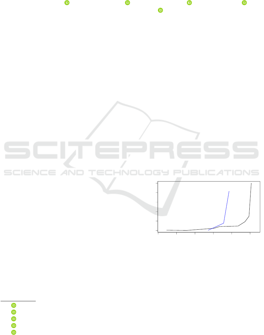
tasks. Figure 1 depicts the size of deep learning mod-
els, indicating an exponential increase in the size of
the models, and hence an urge for efficient compu-
tations. A common technique used in training deep
learning models is SGD but the theoretical behaviour
of SGD in rarely studied in low-precision number for-
mats. Although there is a surge of articles on real
numbers (for example see (Polyak, 1967), (Schmidt
et al., 2011), (Ram et al., 2009)), the performance
of SGD in low-precision number formats started re-
cently. Depending on the precision, the loss land-
scape can change considerably. Figure 2, for instance,
a
https://orcid.org/0000-0002-0147-932X
b
https://orcid.org/0000-0002-5704-3170
c
https://orcid.org/0000-0002-9870-9012
d
https://orcid.org/0000-0002-1953-9343
e
https://orcid.org/0000-0001-6673-4224
2012 2014 2016 2018 2020 2022
0 2 4 6 8 10
Date
Number of Parameters (Billions)
AlexNet
InceptionV2
AmoebaNet−B
ResNext−101
Bit−M
VIT−G
SwinV2
SEER−RG
Transformer
GPT2
MegatronLM
Figure 1: Exploding trend of deep models for image classi-
fication (black) and language models (blue) in time.
depicts this situation for ResNet-18 loss landscape in
both single-precision and low-precision number for-
mats. Motivated by Figure 2, we present a formal
study of SGD for quasi-convex functions when com-
putations are performed in low-precision number for-
mats.
We note that numerical errors, both in forward
and back propagation, can possibly affect the conver-
gence behaviour of the algorithm. It is conceivable
that the numerical errors should increase as the pre-
542
Cacciola, M., Frangioni, A., Asgharian, M., Ghaffari, A. and Nia, V.
On the Convergence of Stochastic Gradient Descent in Low-Precision Number Formats.
DOI: 10.5220/0011795500003411
In Proceedings of the 12th International Conference on Pattern Recognition Applications and Methods (ICPRAM 2023), pages 542-549
ISBN: 978-989-758-626-2; ISSN: 2184-4313
Copyright
c
 2023 by SCITEPRESS – Science and Technology Publications, Lda. Under CC license (CC BY-NC-ND 4.0)

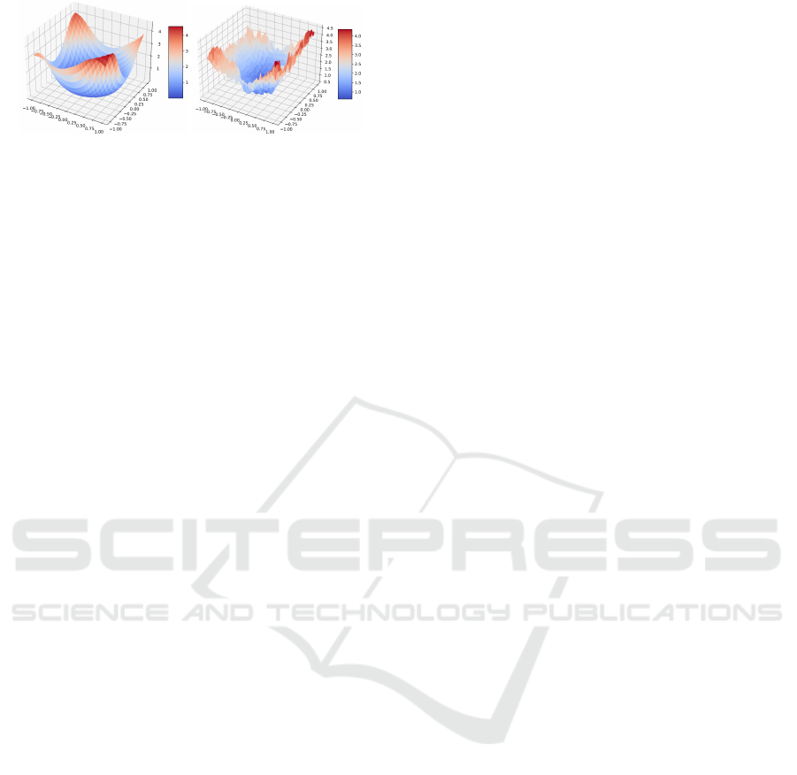
Figure 2: ResNet-18 loss landscape in single-precision
(left) and low-precision number format (right).
cision decreases. To understand the effect of number
format on the convergence of SGD, a careful analysis
of the SGD algorithm for a predetermined precision is
needed. We present both deterministic and stochastic
analysis of the normalized SGD algorithm, obtaining
bounds that show, explicitly, the effect of precision,
i.e. number format. Such bounds can provide guide-
lines as to how SGD convergence is affected when
constraints render performing high-precision compu-
tations impractical, and to what extent the precision
can be reduced without compromising SGD conver-
gence.
Our experiments are performed for logistic regres-
sion on MNIST dataset. They confirm that the tra-
jectory of the loss in low-precision SGD setup has at
least a limit point whose loss value is in the proximity
of the minimum when the numerical errors are rela-
tively small, see Theorem 4.1 and Theorem 4.3.
This paper is organized as follows. Section 2
presents a literature review on the low-precision train-
ing of deep learning models and also provides some
common background for theoretical analysis of SGD.
Section 3 discusses some preliminary notations and
definitions for analysis of quasi-convex loss function
and also the floating point number formats. Section 4
contains the main theoretical results. Section 5 pro-
vides some experimental results that support our the-
oretical results. We conclude in Section 6.
2 RELATED WORKS
Recently, deep learning models provide state-of-the-
art performance in various machine learning tasks
such as computer vision, speech, and natural language
processing (NLP). The size of ImageNet classifica-
tion models after the introduction of AlexNet size is
exploded to 200×, and the size of language models
are getting 10× bigger every year. The recent trend
of deep learning models shows that larger models
such as transformers (Vaswani et al., 2017) and their
variants such as GPT2 (Radford et al., 2019), Mega-
tronLM (Shoeybi et al., 2019), and (Brown et al.,
2020) are easier to generalize on different down-
stream tasks. Moreover, examples of large language
models are included in Figure 1 (blue line) and they
show an increasing trend in number of parameters
over time. A similar trend also appears in vision
models, specially after the advent of vision trans-
formers ((Zhai et al., 2022);(Goyal et al., 2022)) that
beat convolutional neural networks (Mahajan et al.,
2018) on various tasks, see Figure 1 (black line). Al-
though such large models have advantage in terms of
accuracy, they suffer from high computational cost
in their training and inference phases. Moreover,
the high computational complexity of these models
causes high energy consumption and memory us-
age which makes their training and deployment dif-
ficult and even sometimes infeasible. Thus, reducing
the computational complexity of large deep learning
models is crucial.
On the other hand, there has been some efforts
in manually redesigning smaller models with similar
accuracy as large models which often require more
complicated training. In image classification small
models such as MobileNet (Howard et al., 2017)
have a similar accuracy as ResNet (He et al., 2016),
and in language models, DistilBERT (Sanh et al.,
2019) shows close performance to BERT. Mean-
while there have been some efforts in designing mod-
els automatically such as (Liu et al., 2018);(Zoph
et al., 2018). Other methods include those preserv-
ing the baseline model’s architecture while modify-
ing computations e.g. compressing large models us-
ing sparse estimation (Luo et al., 2017);(Ramakrish-
nan et al., 2020);(Furuya et al., 2022), or simplify-
ing computations by running on low-precision num-
ber formats (Jacob et al., 2018);(Wu et al., 2020).
Some researchers are even pushing frontiers by stor-
ing weights and reducing activation to binary (Hubara
et al., 2016) or ternary numbers (Li et al., 2021).
Training large models are compute intensive us-
ing single-precision floating point. This is why hard-
ware manufacturers such as NVIDIA, Google, Tran-
scent, and Huawei started supporting hardware for
low-precision number formats such as Bfloat, float16,
and int8. Recently researchers try to map single-
precision computations on lower bits, see (Zhang
et al., 2020);(Zhao et al., 2021); (Ghaffari et al.,
2022).
Majority of the literature on SGD assumes convex
loss function. We weaken this assumption by con-
sidering quasi-convex class of loss functions that in-
clude convex functions as special case. One of the
first works on quasi-convex optimization is (Kiwiel
and Murty, 1996), where is proven that the gradi-
ent descent algorithm converges to a stationary point.
Later, in (Kiwiel, 2001), the differentiability hypoth-
On the Convergence of Stochastic Gradient Descent in Low-Precision Number Formats
543

esis is removed and the convergence result is shown
using quasi-subgradients. In the case of perturbed
SGD, in (Hu et al., 2015) the authors are able to
deal with bounded biased perturbation on the quasi-
subgradient computation. In a subsequent work (Hu
et al., 2016) analyzed the stochastic setting. Recently,
(Zhang et al., 2022) studied the low-precision SGD
for strongly convex loss functions where the authors
used Langevin dynamics. In comparison, our work
differs in two aspects (i) we assume quasi-convexity,
(ii) our setup adds noise to the SGD and this allows
for less stringent assumptions on the noise and its dis-
tribution.
3 PRELIMINARIES
We start with some preliminary notations about quasi-
convexity and floating point number formats in the
sequel.
3.1 Quasi-Convexity
Definition 3.1. A function f : IR
d
→ IR is said to
be quasi-convex if ∀a ∈ IR, f
−1
[(−∞,a)] = {w ∈
IR
d
| f (w) ∈ (−∞, a)} = S
f ,a
is convex.
Definition 3.2. Given a quasi-convex function f :
IR
d
→IR, the quasi-subgradient of f at w ∈ IR
d
is de-
fined as
¯
∂
∗
f (w) = {g ∈ IR
d
| ⟨g,w
′
−w⟩ ≤ 0, ∀w
′
∈
S
f , f (w)
}
In what follows, the optimal value and optimal
set of a function f on a set Ω are respectively de-
noted by f
∗
and Ω
∗
, i.e. f
∗
= inf
w∈Ω
f (w) and
Ω
∗
= argmin
w∈Ω
f (w).
Definition 3.3. Let p > 0 and L > 0. f : IR
d
→ IR
is said to satisfy the H
¨
older condition of order p with
constant L if
f (w) − f
∗
≤ L[dist(w, Ω
∗
)]
p
where dist(w,w
′
) = min
w
′
∥w −w
′
∥ where ∥·∥ de-
notes the Euclidean norm.
The standard theory of SGD convergence relies on
convex or even strict convex assumption on the loss
function. Clearly quasi convex assumption is a gener-
alization of convex assumption, i.e. all quasi convex
functions are convex, but the reverse may not be true.
To further motivate the quasi convex assumption we
show the ResNet-56 loss-landscape projection in two
and three dimensions without skip connections over
the CIFAR10 dataset, see Figure 3. The convex re-
gions and the quasi-convex regions are highlighted.
The quasi-convex regions are larger than the convex
regions. This means that our theory is applicable in a
larger domain of the loss function.
Figure 3: The quasi-convex regions (in green) are larger
than the convex regions (in yellow).
3.2 Floating Points
A base β ∈ N, with precision t ∈ N, and exponent
range [e
min
,e
max
] ⊂ Z define a floating point system
F, where an element y ∈ F can be represented as
y = ±m ×β
e−t
, (1)
where m ∈ Z, 0 ≤m < β
t
, and e ∈ [e
min
,e
max
].
For an x ∈ [β
e
min
−t
,β
e
max
(1 − β
−t
)], let the float
projection function be fl(x) := P
F
(x), then for x,y ∈
F, the rounding error for basic operations op ∈
{+,−,×, /}, is
fl(x op y) = (x op y)(1 + δ
0
), (2)
where the error is bounded by δ
0
≤ β
1−t
.
When trying to compute a subgradient g ∈ ∂ f (w)
for a w ∈ F the error is bounded to
fl(g) = g(1 + δ
1
),
where |δ
1
|≤ cδ
0
and c > 0 depends on the number of
operations needed for computing such subgradient. A
step of subgradient descent in floating point in IR
d
is:
w
k+1
=
{
w
k
−η[g
k
(1 + δ
1k
)]
}
(1 + δ
2k
),
where we suppose η ∈F,
∥
δ
1k
∥
≤cδ
0
√
d and
∥
δ
2k
∥
≤
δ
0
√
d where d is the dimension of δ. We can refor-
mulate it in terms of absolute error
w
k+1
= w
k
−η(g
k
+ r
k
) + s
k
,
and if the norm of the subgradient g
k
and w
k+1
is
bounded, then so are
∥
r
k
∥
≤ R and
∥
s
k
∥
≤ S. Note
that the infinity norm of the errors are bounded
∥δ
1k
∥
∞
≤ cδ
0
, ∥δ
2k
∥
∞
≤ δ
0
,
so
R
2
≤ cδ
0
∥
g
k
∥
, S
2
≤ δ
0
∥
w
k
∥
.
ICPRAM 2023 - 12th International Conference on Pattern Recognition Applications and Methods
544

4 MAIN RESULTS
Although our study is mainly motivated by training
deep learning models and floating point errors, they
can be applied elsewhere.
4.1 Deterministic Analysis
Let P
Ω
(·) be the projection operator over Ω. We start
with adapting and improving the results of (Hu et al.,
2015) in the presence of error in the summation
Theorem 4.1. Let f : IR
d
→ IR be a quasi-convex
function satisfying the H¨older condition of order p
and constant L. Let w
k+1
= P
Ω
(w
k
−η ˆg
k
+s
k
) where
Ω ⊂ IR
d
is compact, c is the diameter of Ω, and
ˆ
g
k
=
g
k
∥g
k
∥
+r
k
, with g
k
∈
¯
∂
∗
f (w
k
), ∥r
k
∥< R < 1, ∥s
k
∥≤ S.
Then
liminf
k→∞
f (w
k
) ≤ f
∗
+ LΓ
p
(c),
where
Γ(c) =
η
2
"
1 +

R +
S
η

2
#
_
"
η
2
(
1 −

R +
S
η

2
)
+ c

R +
S
η

#
.
See the Appendix for the proof.
Remark: Unlike (Hu et al., 2015), decreasing η does
not decrease the error bound always, so we can de-
rive its optimal value by minimizing the bound with
respect to η.
Define
η
1
=
S
√
1 + R
2
, η
2
=
r
S(c −2S)
1 −R
2
, η
3
=
c −S
R
Corollary 4.1.1. The optimal choice for the step size
η that minimizes the error bound in Theorem 4.1 is
reached in at least one of this 3 points {η
1
,η
2
,η
3
}.
The next result presents a finite iteration version of
the previous result. The effect of the number of itera-
tions K, and the starting point w
0
are clearly reflected
in the bound for min
k<K
f (w
k
).
Theorem 4.2. Let f : IR
d
→ IR be a quasi-convex
function satisfying the H¨older condition of order p
and constant L. Let w
′
k+1
= w
k
−η
ˆ
g
k
and w
k+1
=
w
′
k+1
+ s
k
where
ˆ
g
k
=
g
k
∥
g
k
∥
+ r
k
, where g
k
∈
¯
∂
∗
f (w
k
),
∥r
k
∥ < R, ∥s
k
∥ ≤ S. Then,
min
k<K
f (w
k
) ≤ f
∗
+ L

Γ(c
0
) +
c
0
2ηK

p
,
with c
0
= ∥w
0
−w
∗
∥.
See the Appendix for the proof.
4.2 Stochastic Analysis
Here, we present the stochastic counterpart of Theo-
rem 4.1. The theorem requires only mild conditions
on the first two moments of the errors. We start by
defining the notion of stochastic quasi-subgradient.
Definition 4.1. Let w and w
′
be d-dimensional
random vectors defined on the probability space
(W ,F ,P ) and f : IR
d
→ IR be a measurable quasi-
convex function. Then g(w) is called a unit
noisy quasi-subgradient of f at w if ∥g(w)∥
a.s.
= 1
and P

S
f , f (w)
∩A
w
̸=
/
0

= 0, where A
w
= {w
′
:
⟨g(w),w
′
−w⟩ > 0}·
Thus, inspired by results of (Hu et al., 2016), we
prove the following theorem that take into account
both randomness in the gradient and the computation
numerical error.
Theorem 4.3. Let f : IR
d
→IR be a continuous quasi-
convex function satisfying the H¨older condition of or-
der p and constant L . Let w
k+1
= P
Ω
[w
k
−η(
ˆ
g
k
+
r
k
) + s
k
] where Ω is a convex closed set,
ˆ
g
k
is a unit
noisy quasi-subgradient of f at w
k
, r
k
’s are i.i.d.
random vectors with IE
{
r
k
}
= 0 and IE

∥r
k
∥
2

=
dσ
2
r
, and similarly s
k
’s are i.i.d random vectors with
IE
{
s
k
}
= 0 and IE

∥s
k
∥
2

= dσ
2
s
. Further assume
that
ˆ
g
k
, s
k
, and r
k
are uncorrelated. Then,
liminf
k→∞
f (w
k
) ≤ f
∗
+ L

η
2
(1 + dσ
2
r
) +
dσ
2
s
2η

p
a.s.
See the Appendix for the proof.
Similar to Corollary 4.1.1 one can derive the opti-
mal step size.
Corollary 4.3.1. The optimal step size η that min-
imizes the error bound in Theorem 4.3 is η
∗
=
r
dσ
2
s
dσ
2
r
+1
.
Remark: It immediately follows the optimal step size
is
σ
s
σ
r
for large d.
The theorems indicate that the upper bounds in-
crease with S and R, reflecting the effect of accumu-
lation and multiplication errors respectively. Smaller
number formats clearly lead to greater values of S and
R. As for η, the step size, there is a tradeoff. To make
sure that the bounds provide useful information for
practical purposes, one should choose the step size
such that
S
η
(
σ
s
η
) is controlled. This essentially means
that more accuracy is required for smaller step sizes.
On the Convergence of Stochastic Gradient Descent in Low-Precision Number Formats
545

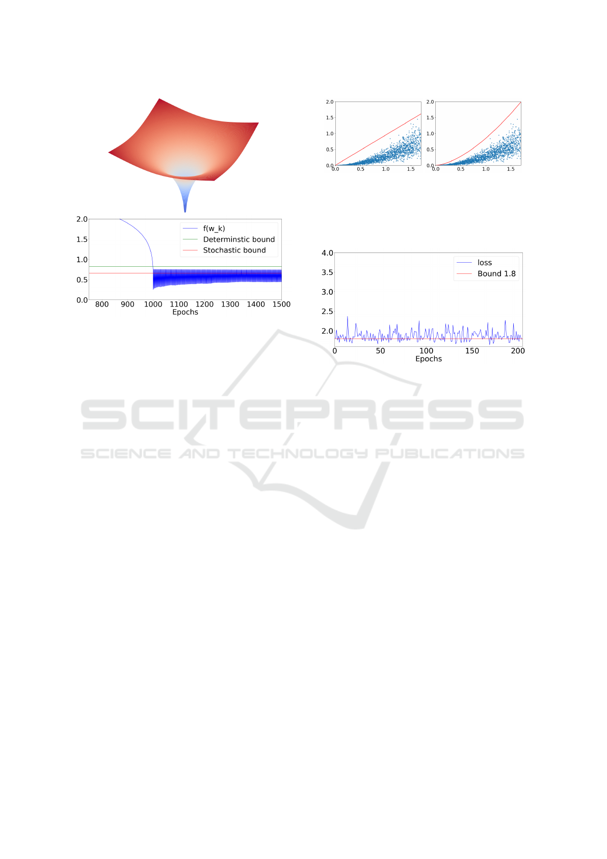
Figure 4: A two dimensional
∥
w
∥
0.2
quasi-convex function
(top panel), and the SGD trace plot confirming the stochas-
tic and deterministic bounds hold (bottom panel).
5 EXPERIMENTS
We performed two types of experiments, a simple
quasi-convex function and a logistic regression on
MNIST dataset.
5.1 Simple Quasi-Convex Function
To asses the bounds obtained in our theorems we
start with a simple quasi-convex function that exactly
satisfy the Holder’s condition. We chose f (w) =
3∥w∥
0.2
where w ∈ IR
40
. In this example, the param-
eters of Holder’s condition are p = 0.2 and L = 3.
We added noise to the gradients and to the weight
update denoted by ∥r
k
∥ and ∥s
k
∥ respectively. This
noise has a uniform distribution r
ki
∼ U(−B
r
,B
r
),
and s
ki
∼ U(−B
s
,B
s
). Figure 4 shows the stochas-
tic and deterministic bound for this experiment. Note
that, the theoretical bounds holds in both stochastic
and deterministic cases.
5.2 Logistic Regression
Here, we present experimental results of logistic re-
gression on the first two principal components of
MNIST dataset. For this experiment, we need to esti-
mate the parameters of the Holder’s condition for the
loss function in order to compute the bounds. To do
so, the Holder’s parameters p and L are manually fit-
ted to the loss function that is evaluated at different
Figure 5: The Holder’s parameters p and L are manually
fitted to the loss function that is evaluated at different dis-
tances from the optimal point. The left panel is a linear fit
with p = 1 and L = 0.95. The right panel demonstrate the fit
with p = 1.6 and L = 0.85. We used p = 1.6 and L = 0.85
for our experiments.
Figure 6: Logistic regression trained using single-precision
SGD and a fixed learning rate.
distances from the optimal point, see Figure 5. The
optimal point w
∗
in our experiments is obtained using
single-precision floating point gradient descent (GD)
method and is used as a reference to compute the pa-
rameters of the bounds f
∗
and c.
Computation of the gradients involves inner prod-
ucts that are computed by multipliers and accumula-
tors. The accumulator have numerical error relative
to its mantissa size. We tested our logistic regression
setup using Bfloat number format and reduced accu-
mulator size. Also note that according to Theorem
4.3, the values of dσ
2
s
and dσ
2
r
are required to com-
pute the bounds. Thus, in our experiments, we used
empirical values of those parameters to compute the
bounds. Also note that we did not plot the determin-
istic bounds for these experiments as they are too pes-
simistic.
In order to evaluate the Holder’s condition param-
eters, p and L, estimated as shown in Figure 5, we use
a single-precision SGD to confirm if the bounds hold.
Figure 6 demonstrates that the loss trajectory (blue
line) has a limit point in the proximity of the optimal
point of the convex loss function. Figure 7 demon-
strates the loss trajectory when both weight update
and gradient computations are performed using Bfloat
number format. Note that Bfloat has 8 bit exponent
and 7 bit mantissa and is used recently to train deep
learning models. The computations are performed us-
ing 15-bit accumulator mantissa. Figure 8 shows the
ICPRAM 2023 - 12th International Conference on Pattern Recognition Applications and Methods
546

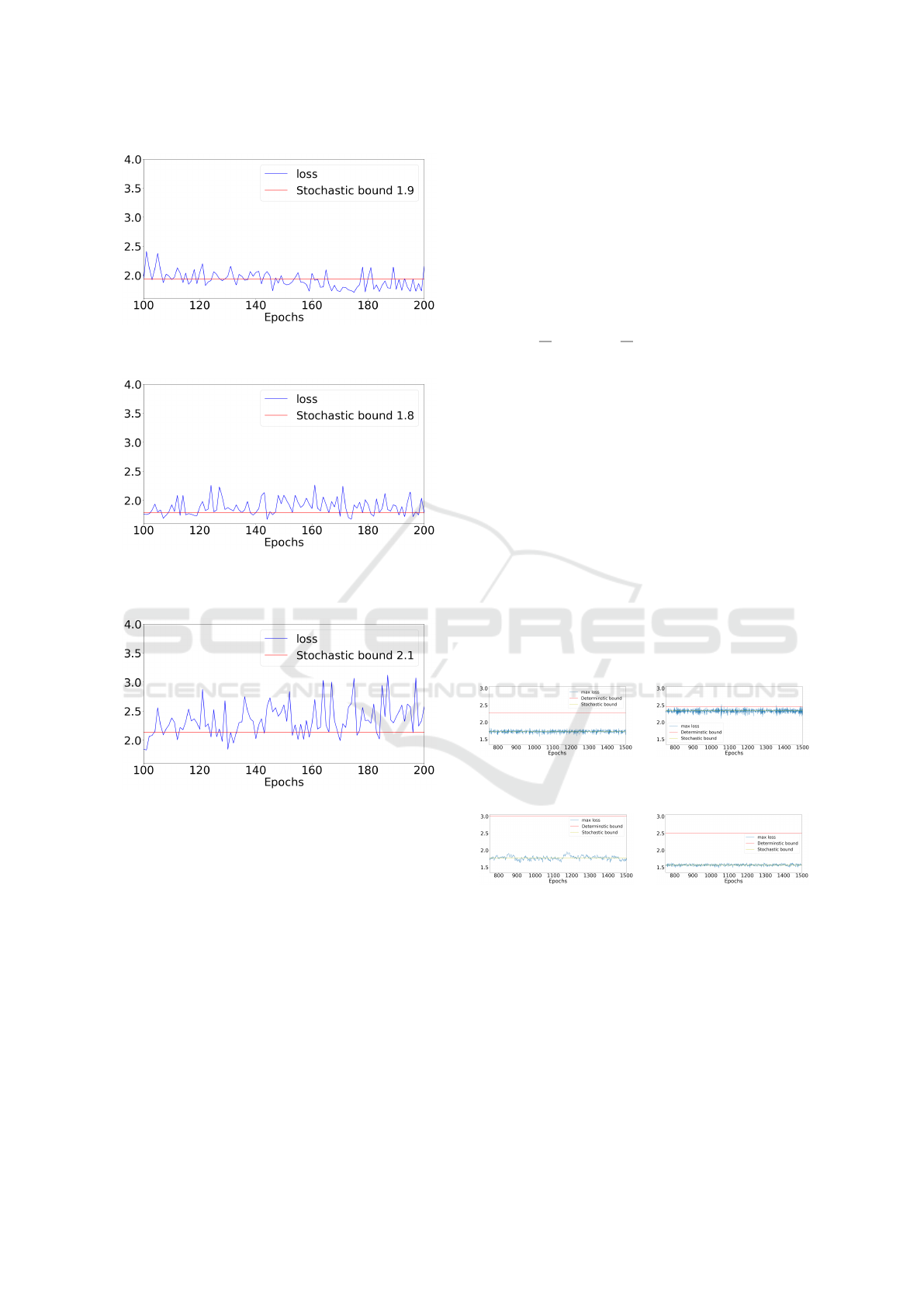
Figure 7: Logistic regression trained using Bfloat SGD with
accumulator size of 15 (s
k
̸= 0 and r
k
̸= 0).
Figure 8: Logistic regression trained using Bfloat gradients
with accumulator size of 15, and single-precision weight
update (s
k
= 0 and r
k
̸= 0).
Figure 9: Logistic regression trained using Bfloat gradients
with accumulator size of 10, and single-precision weight
update (s
k
= 0 and r
k
̸= 0).
loss trajectory when the weight update is in single pre-
cision and only gradient computations are performed
using Bfloat number format. In this experiment, the
stochastic bound is numerically equal to the single-
precision SGD, indicating that the precision of weight
update is more important compared to the precision of
the gradients.
Reducing the accumulator mantissa size has a di-
rect effect on the convergence of SGD. Figure 9 shows
that stochastic bound is increased in the case of 10-
bit accumulator size. In this experiment, the loss tra-
jectory oscillates more in the neighbourhood of the
optimum point. This indicates the accumulator size
plays an important role in reducing the numerical er-
rors of the low-precision SGD computations, and con-
sequently improves the convergence of SGD.
We used the Normalized Gradient Descent (NGD)
algorithm to perform the experiments with the deter-
ministic function f (w) = ∥w∥
0.2
presented in Sec-
tion 5. The maximum number of epochs is set to
1500. Different values for C
0
, B
r
, B
s
and learn-
ing rates were used. The errors, which are manu-
ally added, have uniform distribution in each coor-
dinate. Thus, the variances required in Theorem 4.3
are σ
2
r
=
B
2
r
3
and σ
2
s
=
B
2
s
3
. For the computation of the
bound in Theorem 4.1, c = C
0
was used.
5.3 Optimal Learning Rate
We performed experiments with fixed values for B
s
,
B
r
, but different choices of η to acquire the optimal
choice η
∗
given by Corollary 4.3.1 . The experi-
ment is repeated 10 times, for each tested value of η,.
Finally, the maximum loss function value observed
across all the experiments with the same η is plotted
at each epoch.
The results with B
r
= B
s
= 0.1 are shown in Fig-
ure 10 and Figure 11. The loss trajectory (blue line)
observed with the value suggested by Corollary 4.3.1,
η = 0.0348, is the trajectory that has the lowest level
. Our theorems correctly predict that decreasing the
value of η is sometimes not beneficial in terms of con-
vergence, see Figure 11.
Figure 10: Results with η = 0.1 (left panel) and η = 0.5
(right panel).
Figure 11: Results with η = 0.01 (left panel) and η =
0.0348 (right panel), decreasing the value of η leads to
worse bound and worse convergence.
5.4 MNIST Image Classification
In this section the results obtained on the original
MNIST dataset are reported. In contrast to the ex-
periments in the main body of the manuscript, PCA is
not used to reduce the size of the inputs.
Figure 12 demonstrates that the loss trajectory
(blue line) has a limit point in the proximity of the
optimal point of the convex loss function. Figure 13
On the Convergence of Stochastic Gradient Descent in Low-Precision Number Formats
547

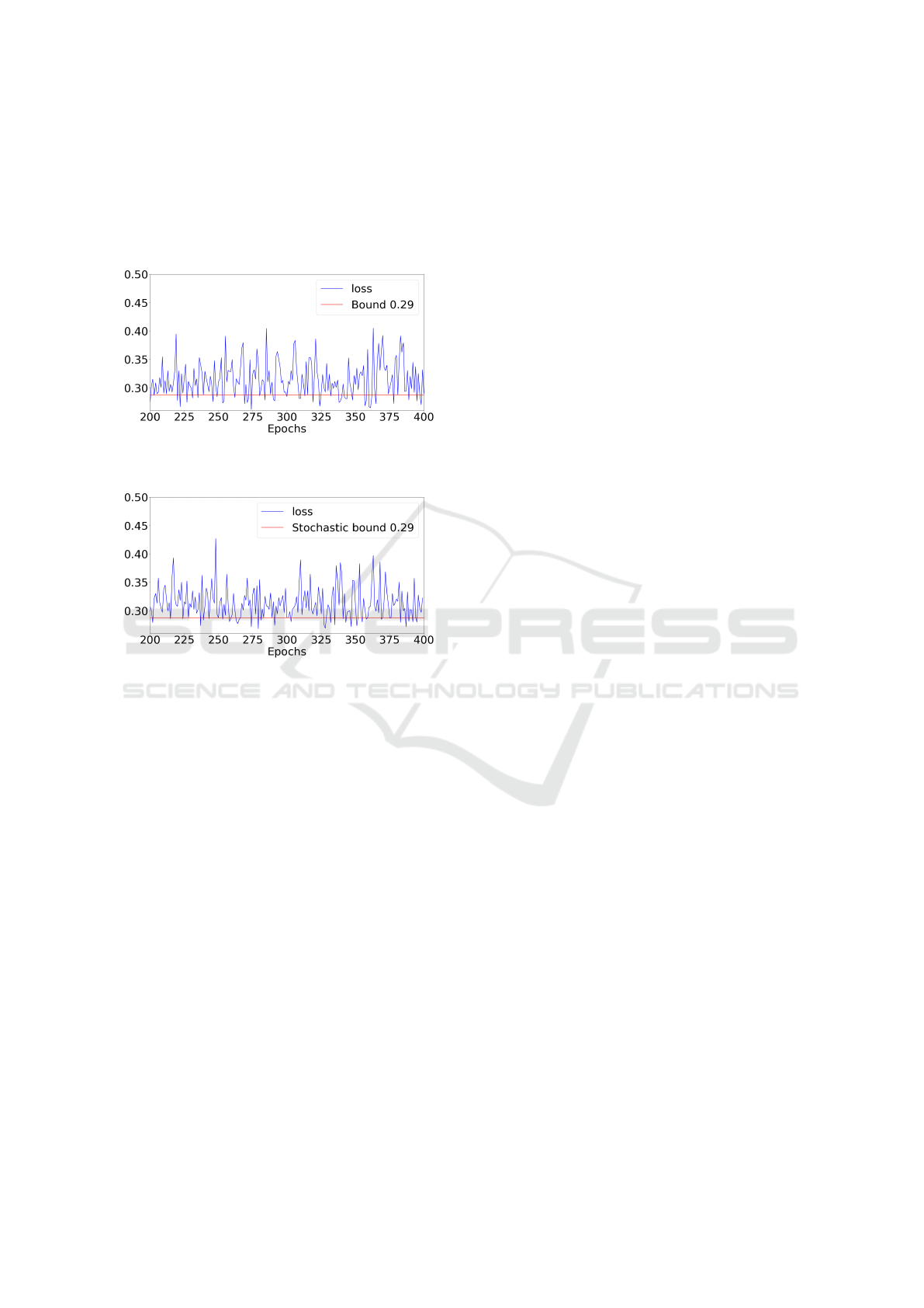
shows the loss trajectory when the weight update is in
single precision and only gradient computations are
performed using Bfloat number format. In this ex-
periment, the stochastic bound is numerically equal
to the single-precision SGD, confirming what already
observed in Figure 8.
Figure 12: Logistic regression trained using single-
precision SGD and a fixed learning rate.
Figure 13: Logistic regression trained using Bfloat gra-
dients with accumulator size of 50, and single-precision
weight update (s
k
= 0 and r
k
̸= 0).
6 CONCLUSION
We have studied the convergence of low-precision
floating-point SGD for quasi-convex loss func-
tions and extended some existing deterministic and
stochastic bounds for convex loss functions. In our
theoretical setup, we considered numerical errors for
weight update and gradient computations. We have
also derived the optimal step size as a corollary of our
theoretical results. Furthermore, in our experiments,
the effect of numerical errors on weight update and
gradient computations are demonstrated. Our experi-
ments show that the accumulator mantissa size plays
a key role in reducing the numerical error and im-
proving the convergence of SGD. Although our ex-
periments with logistic regression are promising, ex-
tension of the experiments for more complex models
is an appealing direction as the future work.
REFERENCES
Brown, T., Mann, B., Ryder, N., Subbiah, M., Kaplan, J. D.,
Dhariwal, P., Neelakantan, A., Shyam, P., Sastry, G.,
Askell, A., et al. (2020). Language models are few-
shot learners. Advances in neural information pro-
cessing systems, 33:1877–1901.
Furuya, T., Suetake, K., Taniguchi, K., Kusumoto, H.,
Saiin, R., and Daimon, T. (2022). Spectral pruning
for recurrent neural networks. In International Con-
ference on Artificial Intelligence and Statistics, pages
3458–3482. PMLR.
Ghaffari, A., Tahaei, M. S., Tayaranian, M., Asgharian,
M., and Partovi Nia, V. (2022). Is integer arithmetic
enough for deep learning training? Advances in Neu-
ral Information Processing Systems. to appear.
Goyal, P., Duval, Q., Seessel, I., Caron, M., Singh, M.,
Misra, I., Sagun, L., Joulin, A., and Bojanowski, P.
(2022). Vision models are more robust and fair when
pretrained on uncurated images without supervision.
arXiv preprint arXiv:2202.08360.
He, K., Zhang, X., Ren, S., and Sun, J. (2016). Deep resid-
ual learning for image recognition. In Proceedings of
the IEEE conference on computer vision and pattern
recognition, pages 770–778.
Howard, A. G., Zhu, M., Chen, B., Kalenichenko, D.,
Wang, W., Weyand, T., Andreetto, M., and Adam,
H. (2017). Mobilenets: Efficient convolutional neu-
ral networks for mobile vision applications. arXiv
preprint arXiv:1704.04861.
Hu, Y., Yang, X., and Sim, C.-K. (2015). Inexact sub-
gradient methods for quasi-convex optimization prob-
lems. European Journal of Operational Research,
240(2):315–327.
Hu, Y., Yu, C., and Li, C. (2016). Stochastic subgradi-
ent method for quasi-convex optimization problems.
Journal of nonlinear and convex analysis, 17:711–
724.
Hubara, I., Courbariaux, M., Soudry, D., El-Yaniv, R., and
Bengio, Y. (2016). Binarized neural networks. Ad-
vances in neural information processing systems, 29.
Jacob, B., Kligys, S., Chen, B., Zhu, M., Tang, M., Howard,
A., Adam, H., and Kalenichenko, D. (2018). Quan-
tization and training of neural networks for efficient
integer-arithmetic-only inference. In Proceedings of
the IEEE conference on computer vision and pattern
recognition, pages 2704–2713.
Kiwiel, K. and Murty, K. (1996). Convergence of the steep-
est descent method for minimizing quasiconvex func-
tions. Journal of Optimization Theory and Applica-
tions, 89.
Kiwiel, K. C. (2001). Convergence and efficiency of
subgradient methods for quasiconvex minimization.
Mathematical Programming, 90:1–25.
Li, X., Liu, B., Yu, Y., Liu, W., Xu, C., and Partovi Nia,
V. (2021). S3: Sign-sparse-shift reparametrization for
effective training of low-bit shift networks. Advances
in Neural Information Processing Systems, 34:14555–
14566.
ICPRAM 2023 - 12th International Conference on Pattern Recognition Applications and Methods
548

Liu, H., Simonyan, K., and Yang, Y. (2018). Darts:
Differentiable architecture search. arXiv preprint
arXiv:1806.09055.
Luo, J.-H., Wu, J., and Lin, W. (2017). Thinet: A filter level
pruning method for deep neural network compression.
In Proceedings of the IEEE international conference
on computer vision, pages 5058–5066.
Mahajan, D., Girshick, R., Ramanathan, V., He, K., Paluri,
M., Li, Y., Bharambe, A., and Van Der Maaten, L.
(2018). Exploring the limits of weakly supervised pre-
training. In Proceedings of the European conference
on computer vision (ECCV), pages 181–196.
Polyak, B. (1967). A general method for solving extremum
problems. Soviet Mathematics. Doklady, 8.
Radford, A., Wu, J., Child, R., Luan, D., Amodei, D.,
Sutskever, I., et al. (2019). Language models are un-
supervised multitask learners. OpenAI blog, 1(8):9.
Ram, S. S., Nedi
´
c, A., and Veeravalli, V. V. (2009). In-
cremental stochastic subgradient algorithms for con-
vex optimization. SIAM Journal on Optimization,
20(2):691–717.
Ramakrishnan, R. K., Sari, E., and Nia, V. P. (2020). Differ-
entiable mask for pruning convolutional and recurrent
networks. In 2020 17th Conference on Computer and
Robot Vision (CRV), pages 222–229. IEEE.
Sanh, V., Debut, L., Chaumond, J., and Wolf, T. (2019).
Distilbert, a distilled version of bert: smaller, faster,
cheaper and lighter. arXiv preprint arXiv:1910.01108.
Schmidt, M., Roux, N., and Bach, F. (2011). Convergence
rates of inexact proximal-gradient methods for convex
optimization. Advances in neural information pro-
cessing systems, 24.
Shoeybi, M., Patwary, M., Puri, R., LeGresley, P., Casper,
J., and Catanzaro, B. (2019). Megatron-lm: Training
multi-billion parameter language models using model
parallelism. arXiv preprint arXiv:1909.08053.
Vaswani, A., Shazeer, N., Parmar, N., Uszkoreit, J., Jones,
L., Gomez, A. N., Kaiser, Ł., and Polosukhin, I.
(2017). Attention is all you need. Advances in neural
information processing systems, 30.
Wu, H., Judd, P., Zhang, X., Isaev, M., and Micikevicius,
P. (2020). Integer quantization for deep learning in-
ference: Principles and empirical evaluation. arXiv
preprint arXiv:2004.09602.
Zhai, X., Kolesnikov, A., Houlsby, N., and Beyer, L. (2022).
Scaling vision transformers. In Proceedings of the
IEEE/CVF Conference on Computer Vision and Pat-
tern Recognition, pages 12104–12113.
Zhang, R., Wilson, A. G., and De Sa, C. (2022).
Low-precision stochastic gradient langevin dynamics.
In International Conference on Machine Learning,
pages 26624–26644. PMLR.
Zhang, X., Liu, S., Zhang, R., Liu, C., Huang, D., Zhou, S.,
Guo, J., Guo, Q., Du, Z., Zhi, T., et al. (2020). Fixed-
point back-propagation training. In Proceedings of the
IEEE/CVF Conference on Computer Vision and Pat-
tern Recognition, pages 2330–2338.
Zhao, K., Huang, S., Pan, P., Li, Y., Zhang, Y., Gu, Z., and
Xu, Y. (2021). Distribution adaptive int8 quantization
for training cnns. In Proceedings of the AAAI Con-
ference on Artificial Intelligence, volume 35, pages
3483–3491.
Zoph, B., Vasudevan, V., Shlens, J., and Le, Q. V. (2018).
Learning transferable architectures for scalable image
recognition. In Proceedings of the IEEE conference on
computer vision and pattern recognition, pages 8697–
8710.
On the Convergence of Stochastic Gradient Descent in Low-Precision Number Formats
549