Towards Improved Indoor Location with Unmodiﬁed RFID Systems

Rui Santos

1 a

, Ricardo Alexandre

2 b

, Pedro Marques

1 c

, M

ario Antunes

1,2 d

ao Paulo Barraca

1,2 e

, Jo

ao Silva

and Nuno Ferreira

DETI, Universidade de Aveiro, Aveiro, Portugal

Instituto de Telecomunicac¸

oes, Universidade de Aveiro, Aveiro, Portugal

Think Digital, Aveiro, Portugal

Keywords:

Indoor Location, Machine Learning, Passive RFID Tag, Regression Models.

Abstract:

The management of health systems has been one of the main challenges in several European countries, espe-

cially where the aging population is increasing. This led to the adoption of smarter technologies as a means to

automate the processes within hospitals. One of the technologies adopted is active location solutions, which

allows the staff within the hospital to quickly ﬁnd any sort of entity, from key persons to equipment. In this

work, we focus on developing a reliable method for active location based on RSSI antennas, passive tags, and

ML models. Since the tags are passive, the usage of RSSI is discouraged, since it does not vary sufﬁciently

based on our experiments. We explored the usage of alternative features, such as the number of activations per

tag within a time slot. Throughout our evaluation, we were able to reach an average error of 0.275 m which is

similar to existing RSSI IPS.

1 INTRODUCTION

The management of health systems and their eco-

nomic viability, especially in western countries where

the aging population is increasingly signiﬁcant, and

has been one of the main challenges for several Eu-

ropean countries. With an increase in the number

of patients and difﬁculty in making annual budgets

keep up with this growth. Hospitals, as well as other

clinical centers have been looking for new solutions

that enable them to maximize service efﬁciency, re-

duce costs and increase patient satisfaction. To auto-

mate these processes some hospitals have started to

adopt active localization technologies through Radio

Frequency Identiﬁcation (RFID) (Paiva et al., 2018;

Tegou et al., 2018). Using Random Forest (RF) tech-

nologies, it is possible to monitor the movement of pa-

tients through the various hospital sectors, as well as

the location and use of medical equipment, and even

https://orcid.org/0000-0003-2157-7602

https://orcid.org/0000-0001-8836-0139

https://orcid.org/0000-0001-5656-1817

https://orcid.org/0000-0002-6504-9441

https://orcid.org/0000-0002-5029-6191

the stock and supply of medications to patients.

This paper aims to explore solutions based on RF,

for indoor localization of resources. The developed

models have, as requirements, the speed of response,

the accuracy of the location and the lowest volume

of data for each prediction (minimizing the electrical

consumption by parts of the RFID radios). The work

described is part of a research project aiming for a

low-cost indoor location system using commonly ac-

quired RFID antennas and tags.

Ideally one would use RFID based technology

for developing an Indoor Positioning System (IPS).

However, during our experiments RFID technology

with passive tags did not produce enough information

for developing an accurate IPS. The main outcome

of this work is the exploration of alternative features,

that can be used to develop IPS with accuracy levels

similar to traditional ones based on RFID.

The remaining document is organized as follows.

section 2 described the current state of the art for ac-

tive indoor location. The following section (section 3)

describes the hardware used in the execution of this

study. section 4 presents the proposed solution. We

describe the results of our evaluation on section 5. Fi-

nally, the conclusion can be found on section 6.

156

Santos, R., Alexandre, R., Marques, P., Antunes, M., Barraca, J., Silva, J. and Ferreira, N.

Towards Improved Indoor Location with Unmodiﬁed RFID Systems.

DOI: 10.5220/0011793700003411

In Proceedings of the 12th International Conference on Pattern Recognition Applications and Methods (ICPRAM 2023), pages 156-163

ISBN: 978-989-758-626-2; ISSN: 2184-4313

 2023 by SCITEPRESS – Science and Technology Publications, Lda. Under CC license (CC BY-NC-ND 4.0)

2 STATE OF THE ART

In the past two decades, IPS have been increasing in

popularity, due to the wide range of technologies and

value they can provide to multiple business areas.

There are multiple techniques used in location

systems, such as multilateration (Carotenuto et al.,

2019), angulation (Pom

arico-Franquiz et al., 2014),

ﬁngerprinting (Suroso et al., 2021) and others. These

techniques require some information provided by

the antennas and tags used, like the Time of Ar-

rival (ToA) (Shen et al., 2014), Angle of Arrival

(AoA) (Xiong and Jamieson, 2013) and Received

Signal Strength Indication (RSSI) (Hightower et al.,

2001). The tags used in these systems can be active

or passive.

SpotON (Hightower et al., 2001) is a location sys-

tem that uses RSSI to locate active RFID tags in a

three-dimensional space. LANDMARC (Ni et al.,

2003) is a system that also reﬂects the relationship

between RSSI and power levels and makes use of ref-

erence tags and the K-NN algorithm to estimate the

positions. It has an accuracy of 2 m and a location

delay of 7.5 s. In (Suroso et al., 2021) Dwi et al. pro-

pose a ﬁngerprinting based positioning system using

a RF algorithm and RSSI data, which achieved an er-

ror of 0.5 m, which is 18% lower than the compared

Euclidean distance method. In (Chanama and Wong-

wirat, 2018), Lummanee et al. compare the perfor-

mance of a Gradient Boosting algorithm to a typical

Decision Tree (DT) applied in a positioning system.

The experiment was based on a 324 m

area divided

in 9 zones. The DT based Gradient Boosting algo-

rithm achieved an estimation error of 0.754 m for 19

reference radio signals at 50 samples per zone, 17.8%

more accurate than the typical DT. In (Choi et al.,

2009) Jae et al. developed a passive RFID based lo-

calization system which uses RSSI information and

reference tags to predict one-dimensional position of

the asset. It achieves an error of 0.2089 m using the

K-NN technique in a 3 m space.

These methods are mainly based on RSSI, which

has the disadvantage of suffering greatly from attenu-

ation due to internal obstacles and dynamic environ-

ments. Unlike SpotON and LANDMARC, the ap-

proach in (Wilson et al., 2007) by Wilson et al. does

not depend on RSSI, however, is based on the same

RSSI principles. This research work is based on pas-

sive RSSI technology. Two scenarios of stationary

and mobile RSSI tags are considered. The method

gives tag count percentages for various signal atten-

uation conditions. The tags are located by recording

characteristic curves of readings under different atten-

uation values at multiple locations in an environment.

Similarly, Vorst et al. (Vorst et al., 2008) use passive

RFID tags and an onboard reader to locate mobile ob-

jects. Particle Filter (PF) technique is exploited to es-

timate the location from a prior learned probabilistic

model, achieving a precision of 0.20–0.26 m.

3 HARDWARE DESCRIPTION

Given the setting where this work has developed, the

hardware was pre-selected. The hardware consists of

two units (processing + radio), that communicate with

each other through a physical bus (RS232, RS485 or

Ethernet). The local processing unit was designed

to have Long Term Evolution (LTE) and Ethernet

communications support, a 230 V Alternating Cur-

rent (AC) power supply and an Advanced RISC Ma-

chine (ARM) processor running a GNU/Linux oper-

ating system with low power consumption. The an-

tenna model is quite common and is used as provided

by the manufacturer without any custom ﬁrmware.

The use of unmodiﬁed hardware increases the usabil-

ity and availability of the system while reducing its

price. The drawback is that the antenna processing

capabilities or the information that it reports may be

sub-optimal. According to the manufacturer there is

an automatic gain compensation done at the ﬁrmware

level. This is done to allows the detection of the pas-

sive tags. The work we present aims at bringing value

by providing an effective solution, even with unmod-

iﬁed hardware.

Figure 1 presents the smart antenna module used

as well as RFID tags.

The communication between the antenna and the

tags is made through a carrier wave in the 865–

868 MHz (Ultra High Frequency (UHF)) frequency

range as deﬁned in the EN 302 208 v3.2.0

direc-

tive for the European region, and cannot exceed 2 W

emission power. In this way, the antenna controller

allows the RF emission power adjustment 0–300 mW,

allowing readings up to 25 m and writings up to 6 m

according to the manufacturer. The antenna polariza-

tion is circular with a gain of 12 dBi. The controller

uses the Impinj R2000 chipset supporting the EPC C1

GEN2 protocol

, ISO18000-6C

(see Table 1). This

setup should be one of the most commonly used, as

the hardware and chipset are very popular. We see

this as a major contribution from our work, as the out-

put can be applied to a wide set of existing or future,

https://www.etsi.org/deliver/etsi en/302200 302299/

302208/03.02.00 20/en 302208v030200a.pdf

https://www.gs1.org/standards/rfid/uhf-air-interface-p

rotocol

https://www.iso.org/standard/59644.html

Towards Improved Indoor Location with Unmodiﬁed RFID Systems

157

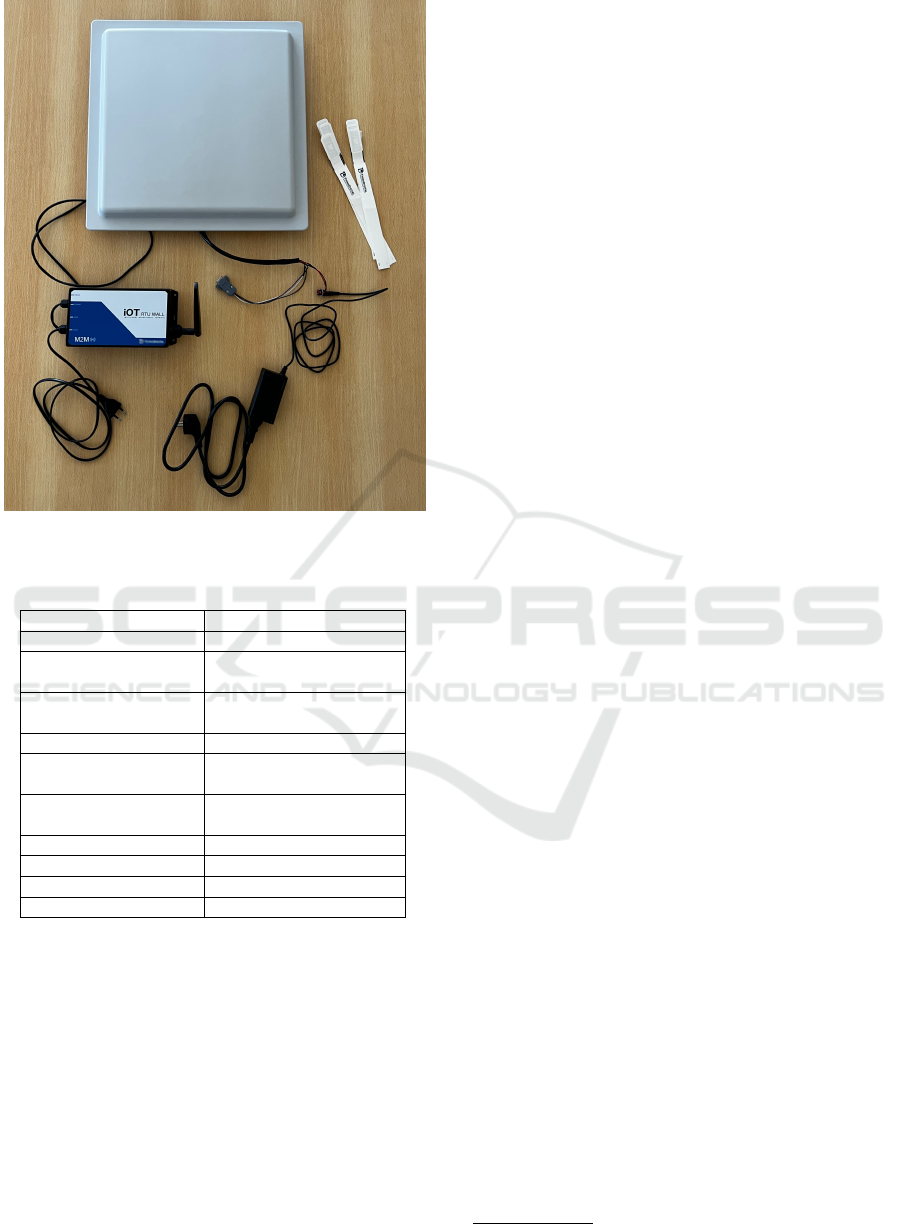
Figure 1: Smart Antenna and passive RFID tags used for

data gathering.

Table 1: Speciﬁcation of the RFID UHF reader and writer.

Product Parameter Parameter Description

Model ACM818A UHF (20M)

Tag Protocol EPC C1 GEN2 /

ISO 18000-6C

Output Power Step interval 1.0dB,

maximum +30dBm

RF Power Output 0.1W - 1W

Built- in Antenna 12dbi linear polarization

Type antenna

Communication Ports 1)RS-232 2)RS-485

3)Wiegand 26 \ 32 bits

Communication Rates 115200bps

Reading/Writing 20m

Multi-tags Reading 200tags/s

Working Voltage DC +12V

deployments.

The real-time communication with the smart an-

tenna is achieved using an MQTT broker, over which

we implemented several control functions: a) Deﬁni-

tion of emission power of the antenna; b) Tag reading

request over a time window (burst); c) Return data ob-

tained at the end of the reading; d) Direct interaction

with an antenna to manage it.

4 PROPOSED SOLUTION

The goal of the Machine Learning (ML) models pro-

posed in this work is to estimate the distance between

the passive tag and the antenna, based on the differ-

ent features collected. This problem can be modelled

as a traditional regression model, the following mod-

els were selected since they represent well-established

and widely used models in the community: i) K-N-

earest Neighbors ii) Decision Tree iii) Random For-

est iv) Support Vector Regressor v) Gradient Boosting

Regressor

The solution was implemented using the Scikit-

learn

library, which is a very popular and robust tool

for RF and statistical modelling in Python. It is im-

portant to mention that we used the default hyperpa-

rameters of each method unless stated in the following

subsections.

The ﬁrst step consists of the analysis and prepa-

ration of the data gathered from the antenna. The

initial solution was developed using single RSSI val-

ues as the input. The features were normalized using

the MinMaxScaler normalization technique. After the

normalization step, the multiple regression algorithms

were trained and evaluated. The output is the distance

(in meters) between the antenna and the RFID tag.

The architecture of the solution is described by Fig-

ure 2.

It is important to mention that the following exper-

iments were conducted in an isolated environment to

ensure the validity of the results. The following sub-

sections present the multiple experiments conducted

in the pursuit of a viable IPS, which is achieved by de-

termining and characterizing the most adequate fea-

tures present in the RFID system.

4.1 Experiment 1

The ﬁrst experimental procedure involved data cap-

ture, using a passive RFID tag placed at several dis-

tances from the RF antenna, obtaining the RSSI val-

ues. Readings were performed from 0.5 m to 5 m,

with 0.5 m increments (distance between the RF an-

tenna and the RFID tag), using different values of

emission power, from 100 mW to 300 mW, during a

predeﬁned time interval of 60 seconds (see Figure 3).

From the result of this ﬁrst experimental proce-

dure, it can be observed that the measured RSSI val-

ues are not proportional to the known distance val-

ues for each reading interval. This happens because

the RF antenna, by default, performs an automatic

compensation of the emission power gains, which

translates into constant average values, unrelated to

https://scikit-learn.org/

ICPRAM 2023 - 12th International Conference on Pattern Recognition Applications and Methods

158

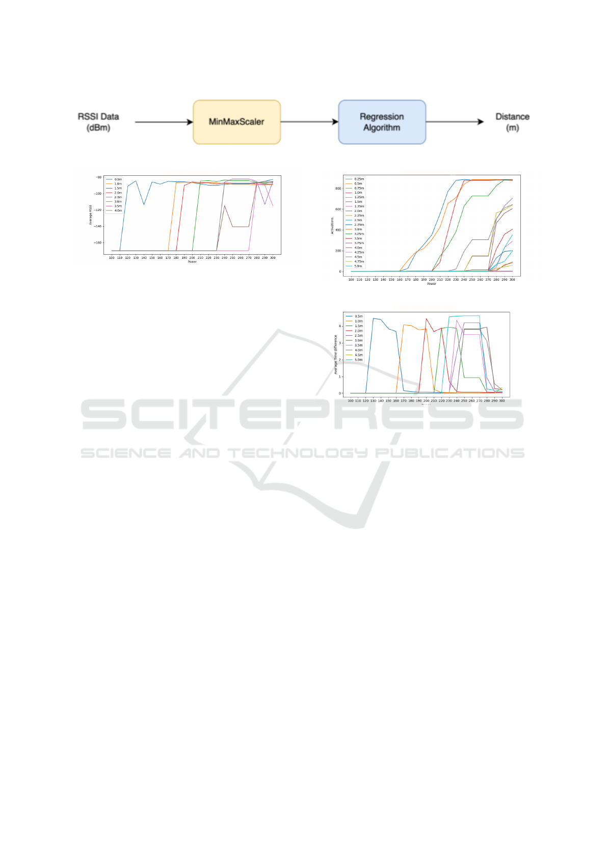
Figure 2: Architecture of the ﬁrst ML solution based on RSSI data.

Figure 3: Average RSSI values from different power levels

and distances.

the known distance values for the passive RFID tags

arranged on site. This strongly diverges from the

vendor-provided information and should be consid-

ered with great care by other researchers. It also

makes it unfeasible to apply ML models over the

RSSI values provided by the hardware.

Due to the fact described above, it was decided

to proceed with the hardware characterization study,

seeking to obtain new feature sets that vary in a mean-

ingful way with the distance. This will be important

for other researchers, as the features can be replicated

over other types of hardware.

4.2 Experiment 2

The second experimental procedure was performed in

the same way as the ﬁrst one, that is, through emission

power scans, between 100 mW and 300 mW. How-

ever, in this case, during shorter pre-deﬁned time in-

tervals (20 seconds), for distance values from 0.25 m

to 5 m, with increments of 0.25 m (distance between

the RF antenna and the RFID tag). The following hy-

pothesis was formulated:

Hypothesis 1. For the same emission power value,

the number of activations registered by the antenna

decreases as the distance increases.

From this second procedure the following results

were obtained (see Figure 4):

By observing Figure 4a, there is a clear increase

in the number of activations as the emission power

increases. It can also be seen that the number of ac-

tivations decreases as the distance increases, for each

power value, validating Hypothesis 1. It can be no-

ticed that the relations are not constant, since the tag

presents a higher number of activations at a distance

of 1 m than at 0.75 m between the powers 220 mW

(a) Number of activations in function of power and distance.

(b) Average time delta between activations in function of

power and distance.

Figure 4: The results for the second experiment.

and 280 mW. This behaviour could be explained by

possible external factors. It can be noted that similarly

to the previous experiment, the number of activations

was purposely kept constant when the power is equal

to 260 mW and 270 mW since the antenna did not reg-

ister activations at these powers.

Figure 4b represents the average time between ac-

tivations (in seconds) for each power and distance

considered. Time peaks between activations can be

veriﬁed for each distance as the power increases.

Since, for a given distance, there are no activations

up to a given power (160 mW for distance 1.0 m), the

average time between activations has been forcefully

set to 0. After activations occur at the ﬁrst few power

levels, this time rises substantially, reaching a peak.

As the emission power increases, there is a decrease

in the average time between activations. It is thus ver-

iﬁed that these peaks occur at higher powers as the

distance increases.

After verifying the experimental results, a second

ML solution was developed to predict the tag distance

from the antenna, according to the number of activa-

tions and the average time between activations, per

scan. However, in this experiment, 10 iterations were

Towards Improved Indoor Location with Unmodiﬁed RFID Systems

159

performed for each power and distance value. This

way, there is more data available for algorithm devel-

opment, the ﬁrst 7 iterations for training and the last

3 for testing. A dataset was generated containing 200

readings, 140 for training and 60 for testing. Figure 5

represents the second solution architecture.

Given the available number of power lev-

els, we applied feature reduction technique,

namely SelectKBest

with the score function

mutual_info_regression. The 200, 280, 290 and

300 power levels are the ones that result in the lowest

error. Table 2 contains the results of the accuracy

of the models for the power levels considered. The

ﬁrst three columns represent the error of the models

trained with all the emission power values and the

last two columns represent just the models trained

with the selected power values. The algorithm that

obtained the lowest error (0.00 m) was K-Nearest

Neighbors (K-NN) with k=1. This model obtained

the same optimal performance for all feature groups,

except when these were only the average number

between activations, where the error was the highest

compared to the other algorithms (0.80 m).

The RF algorithm had, in general, a good perfor-

mance, obtaining in almost all cases the second small-

est error besides K-NN, something that was also ver-

iﬁed in the previous experiment. The Support Vec-

tor Regressor (SVR) proved to be the algorithm with

the worst performance, presenting errors constantly

above 0.58 m for the various groups of features.

It can be seen that models trained only with the

mean time between activations obtained the worst

performance, followed by models trained with both

the number of activations and the mean time between

activations.

The models trained with emission powers of 200,

280, 290 and 300 mW obtained a lower error than the

remaining algorithms trained with all powers, espe-

cially when the features are only the number of ac-

tivations. Thus, it can be concluded that the feature

reduction technique applied had a positive impact on

the algorithms’ performance.

Table 2: RMSE (in meters) for the prediction of the distance

between the tag and the antenna for each group of features.

RMSE Activ. Time All Activ. All

(meters) (4 pwr) (4 pwr)

K-NN 0.00 0.80 0.00 0.00 0.00

SVR 0.58 0.69 0.58 0.58 0.59

GBR 0.31 0.63 0.38 0.13 0.24

RF 0.22 0.64 0.29 0.15 0.21

DT 0.24 0.66 0.66 0.18 0.26

https://scikit-learn.org/stable/modules/generated/skle

arn.feature selection.SelectKBest.html

4.3 Experiment 3

The third experimental procedure was performed in

a larger space, using one dynamic RFID tag and 9

static RFID tags (as references), placed from 1.0 m

to 9 m from the RF antenna (spaced 1 m each). The

emission powers considered in this procedure were

only those that obtained better readings in the previ-

ous procedures, which were 280, 290 and 300 mW,

for distance values from 0.5 m to 10 m, with 0.5 m in-

crements (distance between the RF antenna and the

RFID tag). From this procedure the following graphs

were obtained (see Figure 6):

Figure 6a shows a decrease in the number of ac-

tivations over time. It is also noted that the lower

power (280 mW) obtains a higher number of activa-

tions from 1 m to 2 m, which is unexpected but veri-

ﬁed in the previous experiments.

The number of activations falls sharply until a dis-

tance equal to 4 m, remaining low but not equal to 0

until 5 m and recording a peak at 6 m where the acti-

vations reach 30 for the 300 mW power. Afterwards,

this number remained quite low until 9 m and null for

any power at 10 m.

Figure 6b depicts the average time between acti-

vations. In the ﬁrst distances, the smaller emission

power (280 mW) shows a shorter time between acti-

vations, and this time increases with the increase of

the distance. Although there are no activations for the

powers 280 mW and 290 mW starting at 6 m, the pre-

processing applied to the time between activations

makes this number remain high, thus maintaining the

relationship with the distance.

The graphs presented in Figure 7 show the differ-

ence between the number of activations between the

dynamic tag and the 9 static tags, for each emission

power. It can be seen that, in all graphs, the differ-

ence decreases with distance, as would be expected.

There is a clear relationship between the position of

the static tags and the difference between activations,

as this difference is smaller the closer the static tag is

to the antenna.

In Figure 7a, it can be seen that these remain prac-

tically constant from 4 m on since at this power of

emission there were practically no activations of the

dynamic tag.

5 EVALUATION

Based on the results from the previous experiments

we formulated a second Hypothesis 2:

Hypothesis 2. The difference in the number of activa-

tions between the dynamic tag and the reference tags

ICPRAM 2023 - 12th International Conference on Pattern Recognition Applications and Methods

160

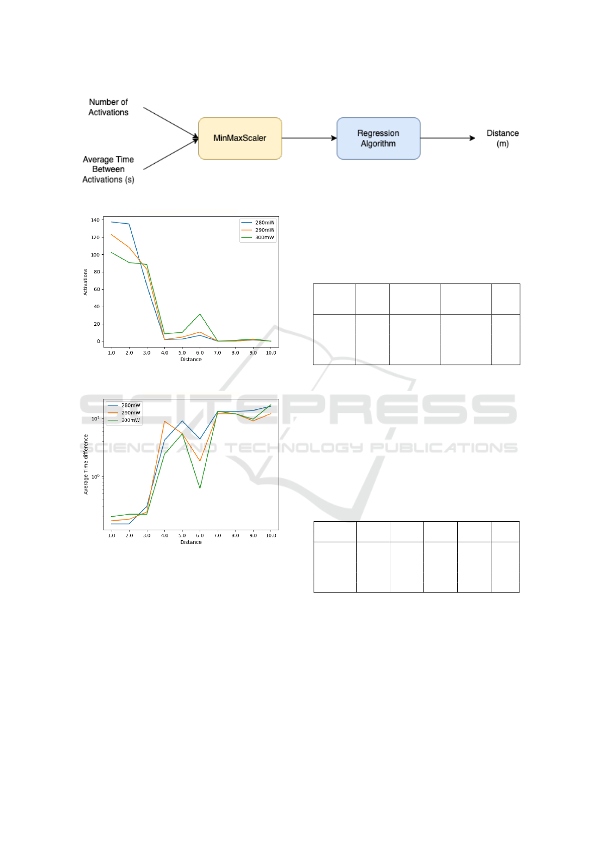
Figure 5: Architecture of the second ML solution based on the number of activations and the average time between activations.

(a) The number of activations for different power levels and

distances.

(b) Average time delta between activations as a function of

power and distance.

Figure 6: The results for the third experiment.

contributes to a performance increase.

A third RF solution was developed using the same

algorithms used in the previous experiments but also

using the difference between the number of activa-

tions. The developed models were trained and tested

using the generated dataset containing 200 readings.

The architecture is described in Figure 8.

The results were recorded in Table 3. The errors

obtained in the tests showed that the models that were

trained with groups of features that included infor-

mation regarding the difference between the number

of activations obtained better performance than those

that did not include this information, validating Hy-

pothesis 2.

Table 3: RMSE (in meters) for the prediction of the distance

between a tag and the antenna, for each group of features.

RMSE Activ. Time Difference All

(meters) between between

activations activations

K-NN 1.19 1.21 0.72 0.72

SVR 1.45 1.26 1.33 1.32

GBR 1.25 0.76 0.84 0.72

RF 1.19 0.85 0.75 0.57

DT 1.48 1.03 1.67 1.08

Several models trained only with the differences

between the number of activations between the dy-

namic tag and the reference tags for each of the three

emission power levels were elaborated. The number

of reference tags and the tags themselves used to train

the algorithms was varied, identifying which combi-

nations result in the lowest error for the various num-

bers considered. The errors for each model tested are

shown in Table 4.

Table 4: RMSE (in meters) for the prediction of the distance

between one tag A and the antenna in experiment 3, using a

set of different reference tags.

RMSE 2 tags 3 tags 4 tags 5 tags All

(meters)

K-NN 0.67 0.60 0.55 0.60 0.72

SVR 1.27 1.37 1.29 1.27 1.33

GBR 0.77 0.76 0.69 0.78 0.84

RF 0.72 0.75 0.72 0.79 0.75

DT 1.08 1.11 1.14 1.74 1.67

Overall, the models that used all the available

features obtained the best performance, followed by

those that used only the difference between the num-

ber of activations. The models trained with only

the average time between activations obtained a per-

formance similar to those that used the difference

between the number of activations, and the models

trained only with the number of activations obtained

the worst performance.

Comparing the different algorithms applied, it can

be seen that SVR obtained the worst performance,

Towards Improved Indoor Location with Unmodiﬁed RFID Systems

161

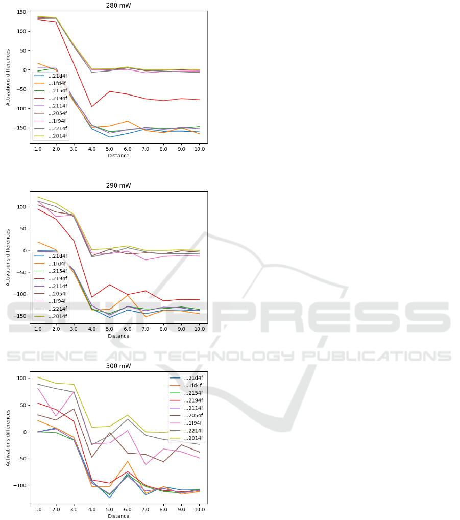
(a) 280 mW.

(b) 290 mW.

Figure 7: The difference of activations recorded for the dy-

namic RFID tag and the reference tags, by reading interval

(20 seconds), for the 280, 290 and 300 mW powers con-

sidered, at different distances, with 0.5 m increments. The

colours shown in the graph correspond to reference tags

placed from 1.0 to 9.0 metres, respectively.

with an error greater than 1.25 m in all tests. The

DT algorithm also did not obtain a good performance,

since the error was always higher than 1 m. The low-

est error was obtained by the RF algorithm (0.57 m)

which obtained a good performance in several tests.

Through Table 4 it is possible to verify that the

smallest error was 0.55 m, obtained by the K-NN al-

gorithm with k=3, using 4 reference tags at 3, 6, 7 and

9 meters away from the antenna. The Gradient Boost-

ing Regressor (GBR) and RF algorithms also obtained

the best performance using this group of features.

From the results obtained in this experiment, it can

be concluded that the use of static reference tags con-

tributes positively to the development of more accu-

rate models.

6 CONCLUSION

The management of health systems has been one of

the main challenges in several European countries,

especially where the ageing population is increasing.

One of the technologies adopted is active location so-

lutions, which allows the staff within the hospital to

quickly ﬁnd any sort of entity, from key persons to

equipment.

In this work, we evaluated the usage of dedicated

hardware (namely the RF antenna) for indoor loca-

tion within a medical environment. Our initial test

showed that RSSI was unreliable as a feature for our

speciﬁc hardware. This happens because the RF an-

tenna, by default, performs an automatic compensa-

tion of the emission power gains, which translates into

RSSI value that does not change with the distance (for

the passive RFID tags arranged on site).

The main contribution of this work is the usage of

alternative features to overcome this issue and achieve

reasonable accuracy with vanilla hardware. The ﬁ-

nal model uses the number of activation and the aver-

age time between activations from a selected range of

power levels as the features for indoor location.

Comparing the results obtained with the systems

studied in section 2, it is possible to conclude that the

accuracy of the developed models is on par without

using RSSI data. It obtained an error of 0.00 m within

a range of 5 m in the second experiment and an error

of 0.55 m within a range of 10 m in the third exper-

iment, resulting in an average error of 0.275 m. The

approach in (Choi et al., 2009) achieves an error of

0.2089 m but within a shorter space of 3 m using RSSI

data.

These results only serve to present an alternative

set of features for speciﬁc hardware, whenever the

typical RSSI metric can not be easily applied. The

ICPRAM 2023 - 12th International Conference on Pattern Recognition Applications and Methods

162

Figure 8: Architecture of the third ML solution based on the number of activations, the average time between activations and

the difference between the number of activations.

proposed features present an adequate level of perfor-

mance. Regardless further testing is required since

the proposed feature can be highly correlated with the

speciﬁc hardware, limiting the deployment of generic

location models.

ACKNOWLEDGEMENTS

This work is supported by the European Regional De-

velopment Fund (FEDER), through the Competitive-

ness and Internationalization Operational Programme

(COMPETE 2020) of the Portugal 2020 framework

[Project SDRT with Nr. 070192 (POCI-01-0247-

FEDER-070192)]

REFERENCES

Carotenuto, R., Merenda, M., Iero, D., and Della Corte,

F. G. (2019). An indoor ultrasonic system for au-

tonomous 3-d positioning. IEEE Transactions on In-

strumentation and Measurement, 68(7):2507–2518.

Chanama, L. and Wongwirat, O. (2018). A comparison of

decision tree based techniques for indoor positioning

system. In 2018 International Conference on Infor-

mation Networking (ICOIN), pages 732–737.

Choi, J. S., Lee, H., Elmasri, R., and Engels, D. W. (2009).

Localization systems using passive uhf rﬁd. In 2009

Fifth International Joint Conference on INC, IMS and

IDC, pages 1727–1732.

Hightower, J., Vakili, C., Borriello, G., and Want, R. (2001).

Design and calibration of the spoton ad-hoc location

sensing system. unpublished, August, 31.

Ni, L., Liu, Y., Lau, Y. C., and Patil, A. (2003). Land-

marc: indoor location sensing using active rﬁd. In

Proceedings of the First IEEE International Confer-

ence on Pervasive Computing and Communications,

2003. (PerCom 2003)., pages 407–415.

Paiva, S., Brito, D., and Leiva-Marcon, L. (2018). Real time

location systems adoption in hospitals–a review and a

case study for locating assets. Acta Scientiﬁc Medical

Sciences, 2(7):02–17.

Pom

arico-Franquiz, J., Khan, S. H., and Shmaliy, Y. S.

(2014). Combined extended ﬁr/kalman ﬁltering for

indoor robot localization via triangulation. Measure-

ment, 50:236–243.

Shen, H., Ding, Z., Dasgupta, S., and Zhao, C. (2014). Mul-

tiple source localization in wireless sensor networks

based on time of arrival measurement. IEEE Transac-

tions on Signal Processing, 62(8):1938–1949.

Suroso, D. J., Rudianto, A. S., Ariﬁn, M., and Hawibowo,

S. (2021). Random forest and interpolation techniques

for ﬁngerprint-based indoor positioning system in un-

ideal environment. International Journal of Comput-

ing and Digital Systems.

Tegou, T., Kalamaras, I., Votis, K., and Tzovaras, D.

(2018). A low-cost room-level indoor localization sys-

tem with easy setup for medical applications. In 2018

11th IFIP Wireless and Mobile Networking Confer-

ence (WMNC), pages 1–7.

Vorst, P., Schneegans, S., Yang, B., and Zell, A. (2008).

Self-localization with rﬁd snapshots in densely tagged

environments. In 2008 IEEE/RSJ International Con-

ference on Intelligent Robots and Systems, pages

1353–1358.

Wilson, P., Prashanth, D., and Aghajan, H. (2007). Utilizing

rﬁd signaling scheme for localization of stationary ob-

jects and speed estimation of mobile objects. In 2007

IEEE International Conference on RFID, pages 94–

99.

Xiong, J. and Jamieson, K. (2013). ArrayTrack: A Fine-

Grained indoor location system. In 10th USENIX

Symposium on Networked Systems Design and Im-

plementation (NSDI 13), pages 71–84, Lombard, IL.

USENIX Association.

Towards Improved Indoor Location with Unmodiﬁed RFID Systems

163