
New Centre/Surround Retinex-like Method for Low-Count Image
Reconstruction
V. E. Antsiperov
a
Kotelnikov Institute of Radioengineering and Electronics of RAS, Mokhovaya 11-7, Moscow, Russian Federation, Russia
Keywords: Low-Count Image Reconstruction, Quantum Noise, Image Perception Quality, Retinex Model, Receptive
Fields.
Abstract: The work is devoted to the issues of synthesizing a new method for low-count images reconstruction based
on a realistic distortion model associated with quantum (Poisson) noise. The proposed approach to the
synthesis of the reconstruction methods is based on the principles and concepts of statistical learning,
understood as input learning (cf. adaptive smoothing). The synthesis is focused on a special representation of
images using sample of counts of controlled size (sampling representation). Based on the specifics of this
representation, a generative model of an ideal image is formulated, which is then concretized to a probabilistic
parametric model in the form of a system of receptive fields. This model allows for a very simple procedure
for estimating the count probability density, which in turn is an estimate of the normalized intensity of the
registered radiation. With the help of the latter, similarly to the scheme of wavelet thresholding algorithms, a
procedure for extracting contrast in the image is built. From the perception point of view, the contrast carries
the main information about the reconstructed image, so such a procedure would provide a high image
perception quality. The contrast extraction is carried out by comparing the number of counts in the centre and
in the concentric surround of ON/OFF receptive fields and turns out to be very similar to wavelet thresholding.
1 INTRODUCTION
Image reconstruction usually refers to the problem of
converting sparse or incomplete data, such as, for
example, radiation counts (readings) from computed
tomography scans, into a readable and usable image.
More generally, image reconstruction involves
transforming some dataset that is difficult to interpret
into an easier-to-interpret target image, where the
target image is some physical property (reflectance,
illumination, absorption), that can be a proxy for the
layout and/or shape of any objects (Aykroyd, 2015).
With the development of imaging technology (in
various radiation ranges, including terahertz, infrared,
X-ray), as well as with the increase in memory
capacity and data processing speed of both
conventional computers and specialized processors,
interest in image reconstruction methods is growing
rapidly. Biomedicine is a clear illustration of this.
Image reconstruction is used now in all popular
medical imaging techniques: magnetic resonance
imaging (MRI), computed tomography (CT),
a
https://orcid.org/0000-0002-6770-1317
radiography (X-ray scanning), etc. At the same time,
since the diagnostic decisions and patient treatments
are often based on digital images, the requirements
for the quality of reconstruction in medicine are very
high.
The imaging techniques listed above are the
products of very different technologies, so their
resulting images differ a lot. However, recently, more
and more often most of them meet the same problem
– formation of images under the conditions of weak
radiation registration. These conditions can arise for
various reasons: in the THz range – due to the lack of
natural sources; in optical astrophysical imaging –
because of the remoteness of objects; in the X-ray, for
example, in CT – due to the desire to reduce radiation
doses. However, since all these radiation types have a
common physical (electromagnetic) nature, there are
also common features that manifest themselves in the
case of low intensities for all ranges. Namely, in all
ranges, the weak radiation acquires a quantum
character and the registration process – image
forming – is carried out in the form of registration of
Antsiperov, V.
New Centre/Surround Retinex-like Method for Low-Count Image Reconstruction.
DOI: 10.5220/0011792800003411
In Proceedings of the 12th International Conference on Pattern Recognition Applications and Methods (ICPRAM 2023), pages 517-528
ISBN: 978-989-758-626-2; ISSN: 2184-4313
Copyright
c
2023 by SCITEPRESS – Science and Technology Publications, Lda. Under CC license (CC BY-NC-ND 4.0)
517

(photo) counts. A good discussion of various aspects
of low-count images for various ranges and
applications is contained in (Caucci, 2012) (see also
the extensive bibliography there).
A characteristic feature of low-count images is the
grainy structure of their textures. these
distortions are
(Dougherty, 2009). Quantum noise degrades
both spatial resolution and contrast, making images
difficult to interpret. Thus, quantum noise also
reduces the speed and accuracy of image processing,
such as segmentation, contrast enhancement, edge
detection, etc. In a good medical imaging system,
inevitable quantum noise is a major source of random
distortion.
Quantum noise manifests itself in the random
nature of independent discrete counts, which are well
described by the Poisson probability distribution. An
important characteristic of the Poisson distribution is
the fact that the standard deviation of the counts
number is equal to the square root of their intensity
(mean). It follows from this, that quantum noise –
deviation of intensity is not additive with respect to
the signal – intensity (in contrast to the traditional
white Gaussian noise). So, quantum noise
suppression by traditional linear filtering turned out
to be ineffective.
Non-linear adaptive smoothing methods using
median-type filters have proved to be more successful
(Oulhaj, 2012). The general idea of adaptive
smoothing is to apply a versatile averaging that adapts
to local topography of the image. Namely, adaptive
smoothing filters average the image not over the
window, but only over that part of it where the image
values differ from the median, for example, by not
more than a certain threshold. The development of the
ideas of adaptive smoothing has recently taken place
in several strategies. The first direction is the non-
linear filtration, such as homomorphic Wiener,
median and bilateral (Tomasi, 1998) filtering. The
second direction is Perona and Malik approach
(Perona, 1990), known as anisotropic diffusion,
which is based on Partial Differential Equations
(PDE) and attempts to save edges and lines. The third
direction – the total variation (TV) approach goes
back to Rudin and Osher (Rudin, 1992) and is based
on minimizing some energy (penalty) function.
Slightly apart from these three strategies is the fourth
one – the wavelet thresholding (wavelet compression)
technique, proposed by Weaver (Weaver, 1991).
Wavelet thresholding separates additive noise from
the true image in the following three-step framework:
analysis – the input data is transformed to wavelet
scaling coefficients; shrinkage – a threshold is
applied individually to the wavelet coefficients and
synthesis – the denoised version of image is obtained
by back-transforming the modified wavelet
coefficients.
Certain successes have been achieved in some of
the listed strategies. So, it is possible to recommend
special methods for specific applications. But in
terms of universal application to a wide range of
problems, almost all methods show approximately
the same quality of image enhancement. Moreover,
Weickert and colleagues showed that many of these
methods can be reduced to one another, at least within
the framework of their algorithmic realization (Alt,
2020). In this regard, in low-count image
reconstruction, all these methods demonstrate
approximately the same relatively low quality.
It seems that the mediocre quality of the
reconstruction is related to the above noted problem
– modelling of distortions by additive noise. The
transition from the image additive global modelling
in the classical filtration theory to local modelling in
the adaptive smoothing methods really leads to an
increase in the quality, but it does not become
significant. Technically, this is due to the fact that the
minimization of some (mathematical) metric of the
difference between the resulting image and its
original is taken as a quality criterion. The most used
metrics here are the sums of absolute or quadratic
differences between the low-count and reconstructed
images. However, it is well known that the image
distortion perceived by a human cannot be adequately
described by such simple mathematical instruments
(Blau, 2019). Since visual perception is very complex
and subject to many distortion factors, the use of a
simple metric for perception quality is hardly a
promising way.
In this regard, it seems more justified to look for
new approaches to improve the quality of images
starting not from the classical methods of digital
image processing (DiSP), but from a large amount of
data accumulated in the field of psychophysics of
vision (Werner, 2014), (Schiller, 2015). A large
amount of data about the periphery of the visual
system (retina) is systematized within the framework
of the so-called Retinex model, first proposed by
Edwin G. Land (Land, 1971). The modern concept of
Retinex considers the illumination created by natural
or artificial sources of radiation, and the reflectivity
of certain objects that redirect this radiation to
imaging devices (the eye, for example) as the main
physical parameters of visual perception. The
illumination usually varies smoothly over a wide
range, so information associated with this factor is
usually negligible. On the other hand, the sharp
ICPRAM 2023 - 12th International Conference on Pattern Recognition Applications and Methods
518

changes in the reflection coefficient between some
objects and at the objects edges are very informative,
and in a sense constitute the main content of images
for a person.
To date, several types of image contrast
enhancement algorithms based on the Retinex model
are known. These algorithms usually analyze an
image at several scales, extracting a low space
frequency component, interpreted as illumination,
and a high frequency component, interpreted as
reflectivity. Local contrast is enhanced by
compressing the luminance range or by extracting the
reflectance. Among the algorithms implemented in
the spirit of Retinex, we note first of all
Center/Surround Retinex (Jobson, 1997), which
forms an adaptively smoothed log of image and
subtracts it from the log of original image to increase
contrast. The current state of the algorithm including
its application in NN – RetinexNet can be found in
(Hai, 2023).
In this article, we propose a new method for low-
count images reconstruction based on a realistic
distortion model associated with quantum (Poisson)
noise. In contrast to the known approaches listed
above, we propose a fundamentally different one –
the perceptual reconstruction of images based on the
most adequate representation model of the recorded
data for human visual perception (not based on formal
metrics of the difference between low-count and
reconstructed images, such as Least-Squares etc).
Namely, we substantiate our approach on the
previously developed biologically motivated
representation of image by controlled size sample of
counts (sampling representation) (Antsiperov, 2023).
Since sampling representations are random objects,
the proposed approach is fundamentally statistical.
Considering that a complete statistical description of
sampling representation is a product of the probability
distribution densities of individual counts, the goal of
the proposed approach is, in essence, to estimate these
densities. In this regard, it is extremely important to
choose a model of parametric distribution densities
adequate to the features of visual perception. In the
next section we discuss in detail the choice of a
parametric family in the form of a system of receptive
fields and derive a density estimating procedure based
on sampling representations in the proposed
parametric model. Considering that the obtained
density estimate is a random realization of the
normalized radiation intensity, in the last section we
synthesize a procedure for extracting the image
contrast from the density. Contrast extraction is
carried out by comparing the number of counts in the
centre and in the concentric surround of ON/OFF
receptive fields. The procedure turns out to be very
similar to wavelet thresholding (Weaver, 1991), but
there are two differences. Instead of wavelets the
receptive fields are used. Instead of the wavelet
coefficients shrinkage to zero, the centre / surround
counts number shrink to the average value between
them is explored. In this regard, it should be
emphasized once again that the methods and models
proposed below are largely motivated by the
mechanisms of the human visual system (HVS)
(Antsiperov, 2022). The fact that they lead to
procedures analogous to modern digital signal
processing methods, most likely determine their
success.
2 CENTRE/ SURROUND
RETINEX-LIKE MODEL FOR
LOW-COUNT IMAGES
The imaging modalities listed above (MRI, CT, X-
ray, etc.) are based on very different technologies,
deal with significantly different types of images, and
are ultimately intended for different applications.
However, since they all are representatives of the
same electromagnetic radiation, they can be described
by the same (parametric) model by choosing definite
parameters (wavelength/frequency) for each range.
This is also true in the case of weak working
radiation, with the only refinement that the model of
radiation–matter interaction should be more
accurately described in the frames of quantum theory.
The discussion of the adequate model for
detecting weak radiation and its substantiation within
the framework of a semiclassical description can be
found, for example, in (Antsiperov, 2021). The main
feature of this model in comparison with the classical
description is that the registration of weak radiation
forming an image results in a set of random (photo)
counts. Thus, the representation of an image by
counts is essentially random, in contrast to the
classical case, where randomness is associated with
external (additive) noise. The statistical description of
such a representation can be given by using the
concept of an ideal imaging device (Antsiperov,
2023). The latter is a plain array (matrix) of ideal
point detectors (cf. jots – (Fossum, 2020)). So, the
result of registration of the photon flux incident on the
sensitive surface of an ideal imaging device is a set
of counts
, where
, are the
coordinates of the registered photons – random
vectors in some area of the plain
. Note that the
New Centre/Surround Retinex-like Method for Low-Count Image Reconstruction
519
number of registered counts is also a random
variable.
It is easy to show (Antsiperov, 2021) that the
statistics of random is given by the Poisson
distribution with the mean parameter
:
(1)
where is the intensity of radiation incident on the
sensitive surface , is the registration time, is the
ideal imaging device quantum efficiency, is the
Planck’s constant and is some characteristic
radiation frequency. Further, it is relatively easy to
show (Streit, 2010).) that the set of counts
can be statistically described as a probability
distribution of points
of some two-dimensional
inhomogeneous Poisson point process (PPP) with the
intensity function
, proportional to the
registered radiation intensity.
Since the number of counts is a random
variable, the above description is not convenient for
practical use (especially if is large enough).
Therefore, we proposed a representation of low-count
images by sets of random vectors, like a set of Poisson
points, but with a fixed (controlled) total number
. Namely, considering the complete set of counts
of an ideal imaging device as some general
population and making a random sample of counts
from it
, we consider the
latter as the desired representation of the image,
called sampling representation. The statistical
discussion of the sampling from the finite population
can be found in (Wilks, 1962). We have shown
(Antsiperov, 2023) that under the same assumptions
that were used to derive the PPP statistics, the
statistics of a fixed (non-random) size sample
can be given by a conditional (for a given image )
multivariate distribution density of the form:
(2)
where, by means of
, the
indexing of counts, internal for the sampling
representation
, is introduced.
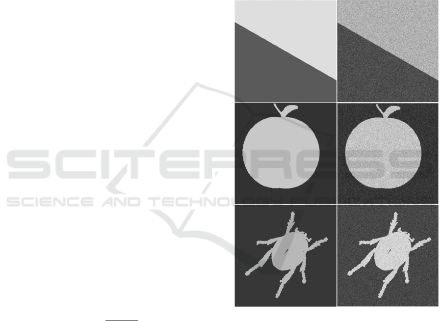
To illustrate typical realizations of random counts
for real images and to prepare sampling
representation examples for further processing, we
generated, in accordance with (2), three sets of
counts: one for simple artificial image (“slope”) and
a pair for images (“apple-1” and “beetle-8”) from the
standard data set MPEG7 Core Experiment CE-
Shape-1 (Latecki, 2000), which are presented in
Figure 1.
All the three images were converted to PNG
format with a color depth of bits (greyscale)
and an image size of pixels.
Wherein only two shades of grey were used for each
image. Counts were generated by the Monte-Carlo
accept-reject method (Robert, 2004) with a uniform
auxiliary distribution
and an auxiliary constant equal to the largest value
of pixels
(see details in (Antsiperov,
2023)).
Figure 1: Image representations by samples of counts
(sampling representations). Left column – source images
“slope”, “apple-1” and “beetle-8” (Latecki, 2000). Right
column – corresponding sampling representations, each
with a size of 3 000 000 counts.
With regard to visual perception, it can be
assumed that the proposed sampling representation of
images is quite consistent with the data recorded by
discrete photoreceptors (rods, cones) at the input of
the visual system – in the outer layer of the retina
(Antsiperov, 2023). At the same time, it is important
to emphasize that the nerve impulses (spikes) sent to
the brain from retina are not the same as the data
ICPRAM 2023 - 12th International Conference on Pattern Recognition Applications and Methods
520

directly recorded by photoreceptors. Retinal ganglion
cells (RGS) – the neurons in the inner layer of retina,
whose axons compose the optic nerve, perform the
retina’s output with the help of numerous
intermediate neurons of the middle and inner layers.
Among them, in addition to bipolar cells that bind
receptors and RGCs from the outer to the inner layer,
horizontal and amacrine cells play an important role,
making horizontal connections in the layers. As a
result, each ganglion cell can receive and process
signals from dozens and sometimes thousands of
receptors. In this regard, it seems that the retina
performs a rather complex processing of input data,
aimed primarily at their optimal compression. Indeed,
if we consider that the number of retinal receptors
reaches ~10
8
, and the number of axons of the optic
nerve is only 10
6
(Schiller, 2015), the amount of input
data is compressed in size by a factor of one hundred.
So, because the retina compresses the input data,
image analysis at higher levels of the visual system
will require its reconstruction. The modern point of
view on the optimization of these related processes is
that the synthesis of the corresponding procedures
should essentially rely on carefully and appropriately
modelling of the available mechanisms / structures.
Explicit use of statistical descriptions and
probabilistic models is the main distinguishing
feature of statistical image reconstruction compared
to classical deterministic methods. Statistical
reconstruction fl
. The key concept
that both descriptions is the Bayes theorem
(Aykroyd, 2015). At the same time, even within the
Bayesian framework, successful approaches can be
developed that differ significantly from each other.
Today, for example, in modern DiSP, an original idea
has been developed that for reconstruction problems
not only traditional methods that a priori model
image parameters (classical Bayesian methods), but
also the methods modelling image features based on
the data of the images themselves (empirical
Bayesian methods) can be successfully used.
(Milanfar, 2013). Further discussion is devoted to the
implementation of this idea in the reconstruction
problem considered.
Since by the image we mean the registered
intensity , the first question of the image
modelling is thus the choice of a model for the
intensity. Let us assume that the intensity can be
modelled by a set of parameters
, which
describe some of its features. Temporarily, without
specifying the content of these features, we assume
that such a -dimensional parametric model
is chosen. According (2), this model can be reduced
to the parametric model of the count probability
distribution
. Thus, the image
encoding (compression) can be reduced to the
parameters
estimation, based on the sampling
representation
, which, again according to
(2), is given by the product of the densities of
individual counts:
(3)
It follows from (3) that for image modelling it is
necessary and sufficient to determine the type of
parametric model
of
distribution density of count. To concretize this
model, it needs, as noted above, to appropriately
adapt it to the known data from the subject area.
Following the initially chosen orientation to the
mechanisms / structures of the visual system, we
formalize for these purposes a perceptually motivated
image model . This model is associated primarily
with the concept of retinal receptive fields (Schiller,
2015), therefore, to substantiate the model, we recall
some basic facts about the mechanisms of neural
encoding at the HVS periphery (retina).
Starting from the works of Hubel and Wiesel in
the 1960s (Hubel 2004), the structure and functions
of retinal receptive fields (RFs) have been studied
quite deeply (Schiller, 2015). The functions and sizes
of individual RFs are determined by the types of
ganglion cells associated with them (retinal output
neurons). The number of types of the latter exceeds
~20, but most of them (~80%) belong to two main
types – midget and parasol cells, each of which has
two subtypes – ON- and OFF-cells. In order not to
overload the discussion, we will further consider only
the family of midget cells encoding the spatial
intensity distribution in the image. Subtypes of ON-
and OFF-cells differ in their response to the nature of
illumination/darkening of the corresponding RFs in
accordance with the central antagonistic structure of
the latter. ON-cells are activated upon stimulation of
the RF center and inhibited upon stimulation of the
concentric surround. Conversely, OFF-cells are
activated upon stimulation of the RF surround and
inhibited upon stimulation of the center (Schiller,
2015). In known mathematical models, the receptive
field of an ON- cell has a center (C) in the form of a
narrow Gaussian profile of spatial activation of
photoreceptors and a wider concentric profile of
inhibition in an antagonistic surround (S); for OFF-
cells, activation and inhibition are reversed. This type
New Centre/Surround Retinex-like Method for Low-Count Image Reconstruction
521
of model is commonly referred to as DoG (difference
of Gaussian) (Cho, 2014).
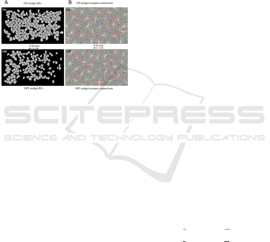
As for the spatial arrangement of the system of
receptive fields, it was found that some pairs of ON-
and OFF-cells have almost completely overlapped
RFs, while the fields of different pairs practically do
not overlap. At the same time, non-overlapping pairs
of adjacent RFs closely adjoin each other, forming a
kind of mosaic that densely fills the entire field of
view of the retina (Gauthier, 2009), see Figure 2.
Figure 2: Locations and shapes of RFs in large populations
of ON- and OFF-midget cells on the retina surface. A) The
RFs of ON- and OFF-cells as a regularly spaced mosaic,
represented by a collection of contour lines. B) The RFs of
ON- and OFF-cell as a connection with the receptors
identified in a single recording of the cell sampling.
Adapted from (Gauthier, 2009) and (Field, 2010).
Based on the previous short overview, we
formalize the parametric model of the family of count
probability densities
as a
mixture of pairs of components
,
:
(4)
where
are positive mixture weights, the
model parameters and mixture components
and
represent compact center and antagonistic
surround of the -th pair of ON/OFF receptive fields.
Components
and
are given by positive
probability distribution densities, having compact
supports
and
, composing in the sum the general
support of the –th RF pair:
:
(5)
If we assume that the supports
and
do not
intersect each other:
, then we can add
the orthogonality-like relations to the normalization-
like equations (5):
(6)
Further, we assume that the set of RF supports
constitutes a partition (mosaic) of the overall
surface of the retina, i.e., all
are pairwise
disjoint, but together they densely cover . This RFs
property causes the components to disappear on all
supports
that do not contain their own
:
(7)
Relations (5, 6, 7) make it very easy to express the
parameters
of the model in terms of
corresponding integrals of the probability density
(4) over the corresponding supports and
thereby clarify the nature of the parameters as the
probabilities of hitting counts to some centres
or
surrounds
of receptive fields:
(8)
Let us make the following remark regarding (8).
Expressions (8) characterize
and
also as the
mean values of the characteristic functions
and
on the surface .
Obviously, expressions (3) cannot be used to find
and
, since the probability density
of
image is not known, but only its sampling
representation
is available. However,
given the number of image counts, one can use the
standard trick, described, for example, in (Donoho,
1994), for estimating the probability density by
wavelet decomposition with empirically formed
coefficients. So, keeping in mind the asymptotic of
the large numbers law and replacing the means of
and
by their sample (empirical) means,
we can approximately write:
(9)
where
and
are the numbers of counts in the
canter and in the surround of the corresponding RFs.
It is easy to show that, within the framework of
the assumptions made (
), the parameters
and
(9) are indeed a probability distribution in
ICPRAM 2023 - 12th International Conference on Pattern Recognition Applications and Methods
522

full accordance with the above interpretation: they all
are non-negative and satisfy the normalization
condition:
.
(10)
where
is the number of counts in
sample
hitting the common support
of the canter and surround of -th RF. Note that
the solutions (9) do not depend at all on the forms of
and
, but only on the forms of their
supports
and
(namely, from the number of
counts that fell into their boundaries). Hence it
follows that for an approximate estimate of the
probability density
(4) only the numbers
and
of counts in the centres / surrounds of the
receptive fields are sufficient. In other words, the
sampling representation
of image can be
reduced in the case considered to occupation number
representation
.
3 CENTRE/SURROUND
RETINEX SHRINKAGE
As noted above, both the chosen model (8) and the
resulting image encoding procedure (9) are very
similar to the wavelet decomposition. In fact, the very
idea of finding the decomposition weights (9) as
sample means was motivated by the Donoho and
Johnstone in work (Donoho, 1994), devoted to
selective wavelet reconstruction.
In this regard, a natural question arises: why,
continuing the noted analogy, not to try applying to
the problem under consideration the most successful
methods from the field of wavelet analysis,
considered as a variant of multiresolution analysis
(Mallat, (1989).)? Of course, the wavelet thresholding
methods (Weaver, 1991) that are extremely popular
today and often cited as wavelet shrinkage methods
(Alt, 2020), should be noted among them first. Thus,
concretizing the previous question, we can formulate
the following problem: considering procedure (9) as
the first step – analysis in some RF thresholding
method – construct its subsequent steps by analogy
with the wavelet shrinkage method (see Introduction).
For this, by the way, there are strong reasons.
Namely, as emphasized in (Chipman, 1997), the main
reason for the use of wavelet shrinkage for some
signal denoising problem is the sparseness of its
underlying set of fine-scale coefficients. That is, if
most of these coefficients are small, and a few
remaining coefficients are large, then only they
explain most of the signal form. By shrinking the
coefficients toward 0, the smaller ones (which contain
primarily noise) may be reduced to negligible levels,
hence denoising the signal. In methods based on the
Retinex model, a similar strategy is utilized – the
local contrast enhancement by compressing smooth
luminance variations and extract sharp changes of the
reflectance. Several successful algorithms (Jobson,
1997) implement this strategy based on
Center/Surround mechanism for estimating the
degree of sharpness of intensity changes. Below, we
propose our own version of a similar approach.
In the frames of approximations (9) made, the
nature of the representation
remains
random, so the density estimation (4) could be still
very noisy. To improve its quality some a priori
information about the parameters (in this
case
) should be used. However, unlike the
method of wavelet compression, based on a simple
additive (linear) model of Gaussian noise, the noise in
our model is multiplicative. These circumstances
significantly complicate the analysis of statistical
relationships and the synthesis of the reconstructing
procedure in the chosen model. Nevertheless, we
succeeded in synthesizing a new Retinex-like
Center/Surround reconstruction method, which has
the form of parameters
correction for
the optimal estimates
calculation to
synthesize the smoothed the count distribution density
(4).
Since the parameters
are independent on
different RFs, the analysis of their statistics can be
carried out independently for all such fields. So, let us
consider some of such fields and denote its non-
negative numbers of counts at center by
and at
antagonistic surround – by
. As this random
numbers have the Poisson distribution, their
expectations are
and
, where is
the intensity of counts at the center of RF, and is the
intensity of counts at surround,
and
are the
areas of the center and surround, so
is
the area of RF support . So, the probabilistic model
of
has the form:
(11)
It follows from (11) that the total number of
counts
is also Poissonian:
(12)
New Centre/Surround Retinex-like Method for Low-Count Image Reconstruction
523

If a priory model of parameters is
,
then overall generative model (joint distribution of
and parameters ) according (11) is:
(13)
Using (12) one can rewrite (13) as
. (14)
We choose a priory model
as a mixture of
two components:
, (15)
where the hyperparameter can be treated as thе
probability of the hypothesis
that and
coincide.
If follows from (15), that marginal
(unconditional) distributions of and are
.
(16)
Note that the marginal distributions (16) do not
depend on the hypotheses
and both are given
by the unconditional distribution .
On the base of (15), (16) we obtain, that
conditional distributions of parameters under
have the form:
.
(17)
As follows from (17), in contrast to (16), the
conditional distributions and do depend on
hypotheses
, since
and
. Nevertheless, it is
interesting that under the hypothesis
the
parameters are still independent.
Substituting model (15) into (13), we obtain the
following expressions for joint distribution
(likelihood function):
.
(
18)
where
– binomial
coefficient,
,
. By
integrating (18) over and from 0 to , we obtain
the (unconditional) joint distribution of
and
:
.
(19)
where probability distribution
of integer is
. (20)
If
is a smooth function at
on a scale ~
, then a good approximation can be written for
distribution (20):
.
(21)
From (18) it follows that conditional joint
distributions of
and
are
.
(22)
So, according to (22), for a given
,
the distribution of numbers
under the
hypothesis
is binomial and under
are
independent.
If with the help of (A.10) we introduce the
likelihood ratio of hypotheses
.
(23)
(18) and (19) will give us the following expression for
the posterior distribution:
. (24)
ICPRAM 2023 - 12th International Conference on Pattern Recognition Applications and Methods
524

Calculating the first moments of distribution (24) in
the usual way, we can obtain the conditional (for a
given
and
/ ) expected values and
of
parameters and . Since the result is, although
simple, but cumbersome expressions, let us use the
assumptions made in the derivation of approximation
(21), which allow us to set
.
and the same for ratios
and
, and write down only the
approximate result:
.
(25)
It follows from (25) that expected values and
are the weighed means of and
or
, which can be interpreted as
average count densities on supports
and
or
of any RF. In two extreme cases – large
and small
expressions (25) for and
are even more
simplified:
. (26)
It follows from (26) that the dominating terms in
the expected
and (25) are essentially determined
by the value of likelihood ratio
(23). When it is
large enough (when the likelihood of hypothesis
is larger than the likelihood of
in
times) both the expected intensities
and are equal
to total number of counts (plus one) divided by the
area of RF base support. Otherwise (when the
likelihood of hypothesis
is smaller than the
likelihood of
in
times) expected
intensities
and are equal to their own ratios
and
.
To simplify the boundary between the above
extreme cases, let us consider the approximation of
(23) in the case
, whence it follows it
also follows that
. So, introducing
the notations
and
,
, putting in these notations
,
, where
, and using
the Stirling formula
, we get:
.
(27)
where approximation (21) was used for
. So, in the case
the criterion
boils down to the test:
.
(28)
where is the Gaussian distribution. After
rearranging the factors and taking the logarithm, the
test (28) becomes:
.
(29)
where
is the estimate of
by the value of
under the assumption that the
is valid and it is
also taken into account that when . If
is almost uniform distribution, then
does not depend on and we can introduce not
depending on threshold:
.
(30)
which is determined by a priori data only.
Taking into account the above simplifications, the
parameters correction problem (36) can be finally
rewritten as:
. (31)
To re-estimate model parameters
,
and
(9), we can use the
above results of Bayesian RF shrinkage as follows
(
):
.
(32)
New Centre/Surround Retinex-like Method for Low-Count Image Reconstruction
525
4 IMAGES RECONSTRUCTION/
SYNTHESIS BASED ON RF
SHRINKAGE
In order to illustrate the potential possibilities of the
proposed approach, we carried out, basing on the
procedure (32), the RF shrinkage of the images shown
in Figure 1 and perform subsequent synthesis.
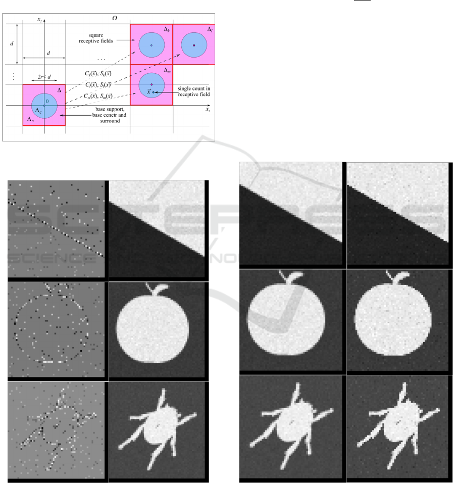
Figure 3: The image surface partition by RF supports
in numerical RF shrinkage procedure implementation.
Figure 4: The contrast (sharp changes in the reflection
coefficient) and smoothed version (slow changes in the
illumination) of Figure 1 images. Left column – contrast
(
), right column – smoothed version (
), see (32).
In the numerical implementation of the procedure
the image field was divided into
square "receptive" fields
, each of sizes
pixels (the original images had, respectively, the sizes
). The center support
of -th RF was
selected as a round area in the center of the field, its
size was determined from the given ratio
of the areas of the center and the RF (i.e. the size of
the cent in pixels was
). The antagonistic
environment was chosen as the addition of the center
to the entire field
. The schematic image
surface partition (mosaic) by RF supports in
numerical procedure implementation is presented in
Figure 3.
Figures 4 shows the extracted from images
contrast
(sharp changes in the reflection
coefficient) of those RFs, where
and their smoothed versions
(slow changes in the illumination) of those RFs,
where
(
).
Figure 5: The comparison of smoothed and synthesised by
RF shrinkage versions of Figure 1 images. Left column –
smoothed version (
), right column – synthesised
version (
), see (32).
ICPRAM 2023 - 12th International Conference on Pattern Recognition Applications and Methods
526

Figures 5 shows the comparison of smoothed versions
(slow changes in the illumination +
smoothed reflection coefficient) of all RFs, and their
synthesised by RF shrinkage versions
(slow
changes in the illumination + sharped changes
reflection coefficient) ( ).
5 CONCLUSIONS
The approach proposed in the article, based on a low-
count image RF shrinking, turned out to be very
promising as it offers new possibilities for synthesis
of real algorithms for nonlinear image reconstruction.
A special representation of images (sampling
representations) developed for these purposes made it
possible, on the one hand, to avoid problems
associated with the size of raster (bitmap)
representations of images, and, on the other hand,
opened wide opportunities for adapting machine
learning methods.
A feature of the proposed approach is the concept
of receptive fields. It provides both good image
quality for human perception and effectively solves
the problems associated with a huge number of
mixture components (4) in the algorithmic
implementation of the reconstruction problem.
We note here that the proposed approach has a
natural extension to the area of parameter
compression methods. As it turned out recently, it has
numerous, non-trivial connections with such areas of
machine learning as anisotropic diffusion methods,
wavelet approaches and variational methods, which
proved to be the best tools in the field of
convolutional neural networks (Alt, 2020).
REFERENCES
Aykroyd, R. G. (2015). Statistical image reconstruction. In
Industrial Tomography, P. 401–427. Elsevier Ltd. DOI:
10.1016/B978-1-78242-118-4.00015-0.
Caucci, L., Barrett, H. H. (2012). Objective assessment of
image quality. V. Photon-counting detectors and list-
mode data. In Journal of the Optical Society of
America. A, Optics, image science, and vision, V. 29(6),
P. 1003–1016. DOI:10.1364/JOSAA.29.001003
Dougherty, G. (2009). Digital Image Processing for
Medical Applications. Springer Science Business
Media. NY. DOI: 10.1007/978-1-4419-9779-1.
Oulhaj, H., Amine, A., Rziza, M., Aboutajdine, D. (2012).
Noise Reduction in Medical Images – comparison of
noise removal algorithms. In 2012 Intern. Conference
on Multimedia Computing and Systems, P. 344–349.
DOI:10.1109/icmcs.2012.6320218.
Tomasi, C, Manduchi, R. (1998). Bilateral filtering for grey
and colour images. In Sixth International Conference
on Computer Vision. 98CH36271.IEEE, P. 839–846.
DOI: 10.1109/ICCV.1998.710815.
Perona, P., Malik, J. (1990). Scale-space and edge detection
using Anisotropic Diffusion. In IEEE Trans on Pattern
Analysis and Machine Intelligence, V. 12, P. 629–639.
Rudin, L. I., Osher, S., Fatemi, E. (1992). Nonlinear total
variation based noise removal algorithms. In Physica.
D, V. 60(1), P. 259–268. DOI: 10.1016/0167-
2789(92)90242-F.
Weaver, J. B., Xu, Y., Healy Jr, D. M., Cromwell, L. D.
(1991). Filtering noise from images with wavelet
transforms. In Magnetic Resonance in Medicine, V.
21(2), P. 288–295. DOI: 10.1002/mrm.1910210213.
Alt, T., Weickert, J., Peter, P. (2020). Translating Diffusion,
Wavelets, and Regularisation into Residual Networks.
// arXiv:2002.02753. DOI:10.48550/arxiv.2002. 02753
Blau, Y., Michaeli, T. (2019) Rethinking Lossy
Compression: The Rate-Distortion-Perception Trade-
off. In Proc. of the 36th International Conference on
Machine Learning, PMLR 97, P. 675–685. DOI:
10.48550/arXiv.1901.07821.
Werner, J.S., Chalupa, L.M. (2014). The new
visual neurosciences. The MIT Press, Cambridge,
Massachusetts.
Schiller, P.H., Tehovnik, E.J. (2015). Vision and the Visual
System. Oxford University Press, Oxford. DOI:
10.1093/acprof:oso /9780199936533.001.0001.
Land, E.H., McCann, J. J. (1971) Lightness and retinex
theory. In Journal of the Optical Society of America, V.
61(1), P. 1–11, 1971, DOI: 10.1364/JOSA.61. 000001.
Jobson, D. J., Rahman, Z., Woodell, G. A. (1997).
Properties and performance of a center/surround
retinex. // In IEEE Transactions on Image Processing,
V. 6(3), P. 451–462. DOI: 10.1109/83.557356.
Hai, J., Hao, Y., Zou, F., Lin, F., Han, S. (2023). Advanced
RetinexNet: A fully convolutional network for low-
light image enhancement. In Signal Processing. Image
Communication, V.112, 116916. DOI: 10.1016/j.
image.2022.116916.
Antsiperov, V., Kershner, V. (2023). Retinotopic Image
Encoding by Samples of Counts. In M. De Marsico et
al. (Eds.): ICPRAM 2021/2022, LNCS 13822, P. 1–24,
Springer Nature, Switzerland AG, DOI: 10.1007/978-
3-031-24538-1_3.
Antsiperov, V. (2021). Maximum Similarity Method for
Image Mining. In ICPR 2021, Part V. Lecture Notes in
Computer Science, V 12665, P. 301-313. Springer,
Cham. DOI: 10.1007/978-3-030-68821-9_28.
Fossum, E. (2020). The invention of CMOS image sensors:
a camera in every pocket. In 2020 Pan Pacific Microel.
Symp., P. 1–6. DOI: 10.23919/PanPacific 48324.
2020.9059308.
Streit, R. L. (2010). Poisson Point Processes Imaging,
Tracking, and Sensing. Springer US: Imprint: Springer.
DOI: 10.1007/978-1-4419-6923-1.
Wilks, S. S. (1962). Mathematical statistics. John Wiley &
Sons, Inc., Hoboken.
New Centre/Surround Retinex-like Method for Low-Count Image Reconstruction
527

Latecki, L. J., Lakamper, R., Eckhardt, T. (2000). Shape
descriptors for non-rigid shapes with a single closed
contour. In Proceedings IEEE Conference on Computer
Vision and Pattern Recognition. CVPR 2000 (Cat.
No.PR00662), V.1, P. 424–429. DOI:
10.1109/CVPR.2000.855850.
Robert, C.P., Casella, G. (2004) Monte Carlo Statistical
Methods, 2nd ed. Springer-Verlag, New York. DOI:
10.1007/978-1-4757-4145-2.
Milanfar, P. (2013). A Tour of Modern Image Filtering:
New Insights and Methods, Both Practical and
Theoretical. In IEEE signal processing magazine, V.
30(1), P. 106–128. DOI: 10.1109/MSP.2011.2179329.
Hubel D.H., Wiesel, T.N. (2004). Brain and Visual
Perception: The Story of a 25-year Collaboration. New
York: Oxford University Press, 2004.
Cho, M.W., Choi, M.Y. (2014). A model for the receptive
field of retinal ganglion cells. In Neural Networks, V.
49, P.51–58. DOI: 10.1016/j.neunet.2013.09.005.
Gauthier, J.L., Field, G.D., et al. (2009). Receptive fields in
primate retina are coordinated to sample visual space
more uniformly. PLoS Biol. V. 7(4), P. e1000063. DOI:
10.1371/journal.pbio.1000063.
Field, G.D., Gauthier, J.L., et al. (2010). Functional
connectivity in the retina at the resolution of
photoreceptors. Nature, V. 467(7316), P. 673–677.
DOI: 10.1038/nature09424.
Donoho, D. L., Johnstone, J. M. (1994) Ideal spatial
adaptation by wavelet shrinkage. In Biometrika, V.
81(3), P. 425–455. DOI: 10.1093/biomet/81.3.425.
Mallat, S. G. (1989). A theory for multiresolution signal
decomposition: the wavelet representation. In IEEE
Transactions on Pattern Analysis and Machine
Intelligence, V. 11(7), P. 674–693. DOI:
10.1109/34.192463.
Sujith, V., Karthik, B. (2022). Removal of noise in Poisson
image based on minimum risk wavelet shrinkage
operator. AIP Conference Proceedings, V. 2426(1).
DOI: 10.1063/5.0111528.
Chipman, H.A., Kolaczyk, E.D., McCulloch, R.E. (1997).
Adaptive Bayesian Wavelet Shrinkage. In Journal of
the American Statistical Association, V. 92(440), P.
1413–1421. DOI: 10.1080/01621459.1997. 10473662.
ICPRAM 2023 - 12th International Conference on Pattern Recognition Applications and Methods
528
