Inverse Rendering Based on Compressed Spatiotemporal Infomation by
Neural Networks
Eito Itonaga, Fumihiko Sakaue and Jun Sato
Nagoya Institute of Technology, Nagoya, Japan
Keywords:
Inverse Rendering, Photometric Stereo, Light Distribution Estimation.
Abstract:
This paper proposes a method for simultaneous estimation of time variation of the light source distribution, and
object shape of a target object from time-series images. This method focuses on the representational capability
of neural networks, which can represent arbitrarily complex functions, and efficiently represent light source
distribution, object shape, and reflection characteristics using neural networks. Using this method, we show
how to stably estimate the time variation of light source distribution, and object shape simultaneously.
1 INTRODUCTION
Inverse rendering, which is the estimation of object
shape, reflection characteristics, and light distribution
from a single image or multiple images, has been ac-
tively studied in the fields of computer graphics as
well as computer vision in recent years. Inverse ren-
dering from a single image is generally regarded as
an ill-posed problem because it requires more infor-
mation than the input information as an image. Even
when multiple images are used as input, it is known
that estimating many unknown parameters such as ob-
ject shape, reflection characteristics, and light source
distribution simultaneously is difficult due to the de-
grees of freedom and representation methods of these
parameters. Therefore, the way these parameters are
represented is very important from the standpoint of
estimation stability.
Therefore, in this study, we focus on the ability
of neural networks to represent arbitrarily complex
functions and represent object shape and light source
distribution using neural networks. This enables all
of the object shapes and light distribution to be rep-
resented as model parameters of the neural network.
By simultaneously optimizing these parameters, we
can simultaneously estimate object shape, reflection
characteristics, and light source distribution from time
series images observed in an environment where the
light source distribution changes over time.
2 RELATED WORKS
Many methods for estimating object shape, reflec-
tion characteristics, and light distribution from im-
ages have been studied. One method for estimating
light distribution from images is based on the diffuse
reflection component on the object’s surface. In this
method, the distribution of light sources is estimated
by expressing the light distribution using a spherical
harmonic function and obtaining the expansion co-
efficients of the spherical harmonic function. How-
ever, the light distribution estimation method based
on diffuse reflections is known to be prone to an ill-
posed problem because high-frequency components
are missing from the image(Marschner and Green-
berg, 1997). In recent years, there have also been
methods that estimate light distribution directly from
images using convolutional neural networks based
on a large amount of training data(Georgoulis et al.,
2018). In addition, the method (LeGendre et al.,
2019) has also been proposed to estimate the light
source distribution by calculating the difference be-
tween the image generated from the estimated light
source distribution and the image actually taken as
a loss and training the network. These methods
have been confirmed to have higher performance than
conventional methods that use physics-based vision.
However, they require the collection of a very large
amount of data in order to perform proper training.
Several methods for estimating object shape and
reflection characteristics have been proposed using
the photometric stereo method, which estimates the
normal vector of the object surface representing the
Itonaga, E., Sakaue, F. and Sato, J.
Inverse Rendering Based on Compressed Spatiotemporal Infomation by Neural Networks.
DOI: 10.5220/0011792200003417
In Proceedings of the 18th International Joint Conference on Computer Vision, Imaging and Computer Graphics Theory and Applications (VISIGRAPP 2023) - Volume 4: VISAPP, pages
467-474
ISBN: 978-989-758-634-7; ISSN: 2184-4321
Copyright
c
 2023 by SCITEPRESS – Science and Technology Publications, Lda. Under CC license (CC BY-NC-ND 4.0)
467

object shape from multiple images taken at different
light source positions(HIGO, 2010). These methods
can simultaneously estimate object shape and reflec-
tion characteristics under conditions where the light
source is known. Similar to light source informa-
tion estimation, a neural network-based method has
also been proposed to simultaneously estimate ob-
ject shape, reflection characteristics, and light dis-
tribution from a single image taken of an indoor
scene(Sengupta et al., 2019). However, this method
also requires a large amount of training data to
achieve appropriate learning.
Therefore, in this paper, we consider the use of
neural networks to represent object shape and light
distribution without using training data and to simul-
taneously estimate object shape, reflection charac-
teristics, and light distribution from time-series im-
ages. This method aims to realize inverse rendering
with properties that are intermediate between physics-
based vision and learning-based vision.
3 OBSERVATION MODEL
3.1 General Rendering Model
First, we discuss the general rendering model. Ren-
dering is the computation of light reflections in a
scene based on specular reflections on object surfaces,
shadows, inter-reflections between objects, etc. The
rendering equation proposed by Kajiya(Kajiya, 1986)
is well-known as a basic mathematical model. There-
fore, rendering in computer graphics corresponds to
solving this rendering equation.
Assuming that no light penetrates into the interior
of the object, the reflectance at the observation point
x as f (x,
⃗
ω,
⃗
ω
′
). This reflectance indicates the ratio
of rays incident from the
⃗
ω
′
direction reflected in the
⃗
ω direction. The angle between the incident direc-
tion
⃗
ω
′
) and the plane normal direction ⃗n is shown by
θ. The set of ray directions incident on point x is de-
noted by Ω. In this case, the observed intensity L
o
is
expressed by the rendering equation as follows:
L
o
(x,
⃗
ω) = L
e
(x,
⃗
ω)+
Z
Ω
f
r
(x,
⃗
ω
′
,
⃗
ω)L
i
(x,
⃗
ω
′
)cosθd
⃗
ω (1)
where L
e
is the amount of light emitted from the point
⃗x. This equation indicates that the observed intensity
is determined by the integral of the reflected light in-
cident from all directions and the light L
e
(x,
⃗
ω) emit-
ted from the object in the
⃗
ω direction. Therefore, the
observed intensity information includes not only the
reflectance characteristics at the point, but also infor-
mation about the surrounding lighting environment.
Therefore, if we can analyze this information appro-
priately, we can reconstruct various types of informa-
tion from the intensity information.
3.2 Intensity Model
Next, we describe the image observation model used
in this study. In equation (1), L
o
is the luminance
emitted from the observation point x on the object sur-
face in the scene in the direction ω, and L
e
is the radi-
ance of light emitted from the object interior. Omega
is the direction of incidence of the light at the obser-
vation point x, which coincides with the hemisphere.
Here, L
e
can be assumed to be zero regardless of the
direction because the light is rarely emitted from the
interior of a typical object. The cosθ, is the just in-
ner product of the normal vector ⃗n and the direction
of incidence
⃗
ω
′
. Thus, the following equation, which
focuses only on the reflection component, is used as
the observation model of the image in this study.
L
r
(x,
⃗
ω) =
Z
Ω
f
r
(x,
⃗
ω
′
,
⃗
ω)L
i
(x,
⃗
ω
′
)(⃗n ·
⃗
ω
′
)d
⃗
ω (2)
When using such an observation model, light distribu-
tion and object shape information for the entire scene,
as well as reflectance property information, are re-
quired to render the image. Conversely, it is possi-
ble to estimate these information from the observed
intensity information.
3.3 Light Distribution Representation
Next, we describe the representation model of light
distribution used in this study. As described in the
equation (2), the light distribution around the object
is necessary to determine the intensity observed on
the object’s surface. However, it is difficult to directly
express this as a continuous quantity. Therefore, the
In this study, we use a geodesic dome as shown in
Fig 1. A geodesic dome is an approximate model of
a sphere composed of triangular patches, which can
discretely represent the spread of points on a sphere.
The vertices are distributed with equal density on the
sphere, so it is possible to represent light distribution
equally at isosceles angles. In this study, we assume
that a point light source exists at the center of gravity
of these triangular patches, and represents light distri-
bution by changing the intensity of each light source.
In this study, the temporal variation of light distribu-
tion is represented by changing the intensity of each
light source on the sphere according to the time.
VISAPP 2023 - 18th International Conference on Computer Vision Theory and Applications
468

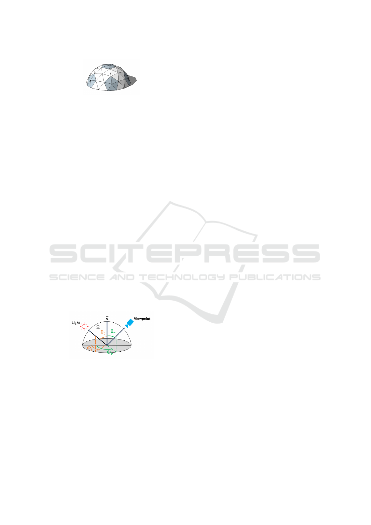
Figure 1: Geodesic Dome.
3.4 Reflectance Model
Next, we describe the representation of reflectance
characteristics used in this study. The BRDF (Bidi-
rectional Reflectance Distribution Function) is a typ-
ical model of the reflectance characteristics of an ob-
ject. The BRDF shows how incident light reflects
from one direction to another on the surface of an ob-
ject in each direction. Therefore, the BRDF can be
used to describe how an object is observed from var-
ious directions under various light sources. Consid-
ering the reflection at the observation point x on the
object surface, the BRDF at the observation point x
depends on the incident direction of light (θ
i
,φ
i
) and
the viewpoint direction (θ
r
,φ
r
), as shown in Figure2.
Although the BRDF is strictly wavelength-specific, it
is often redundant to describe the reflectance of each
wavelength for rendering purposes, so it is common
practice to define a BRDF for each of the three RGB
channels. With the BRDF defined in this way, the ra-
tio of the intensity in the incident direction
⃗
ω
′
to the
intensity in the view direction
⃗
ω at the observation
point x can be described as follows:
f
r
(x,
⃗
ω
′
,
⃗
ω) (3)
By this function f , the reflectance property of the sur-
face can be described.
Figure 2: Directions for BRDF.
4 SIMULTANEOUS ESTIMATION
OF LIGHT DISTRIBUTION
AND SHAPE INFORMATION
Inverse rendering is to obtain the object shape ⃗n, re-
flection property f
r
, and light distribution L
i
in Eq.(2)
from the observed intensity, and the difficulty of the
problem varies greatly depending on the representa-
tion method and degree of freedom. Many of the
methods proposed so far have focused on the fre-
quency characteristics of the light distribution and
used spherical harmonic functions to represent the
light distribution. Such methods have been effective
in light distribution estimation focusing on diffuse re-
flections, in which the reflected components consist
only of low-frequency components. However, in anal-
yses focusing on specular reflections, which contain
higher-frequency components, the number of degrees
of freedom increases significantly when attempting to
represent the high-frequency components of the light
distribution, and this makes the estimation unstable.
Furthermore, when time series information is used,
the number of degrees of freedom increases further,
making stable estimation difficult. Therefore, we pro-
pose a method to simultaneously estimate light dis-
tribution, object shape, and reflection characteristics
from time-series images by using a neural network
that can represent arbitrarily complex functions.
4.1 Definition
Based on the above, we define and formulate the prob-
lem addressed in this paper. In this paper, we take as
input multiple images taken continuously in a situa-
tion where the light source environment changes with
time, and estimate the temporal change of the light
distribution and the shape of the photographed object
from these images. The object shape and light dis-
tribution are represented as a regression using a neu-
ral network. That is, given a certain coordinate on
the light distribution, there is a function that returns
the intensity of the light source. Similarly, for object
shape, given a certain coordinate on the image, there
is a function that returns the normal direction. There-
fore, the estimation of object shape and light distribu-
tion corresponds to training a neural network that can
appropriately represent the input image.
To solve such a problem, Eq.(2) is redefined in
terms of geodesic domes and neural networks. As-
suming that the object-camera relationship is fixed
and the shape of the object does not change with
time, the viewpoint direction in the observed image
can be considered fixed. Assume that T time images
are available as input. Assume that the light distri-
bution at time t(t = 1, 2, ·· · , T ) is sampled using a
geodesic dome with G sampling points as (θ
j
,φ
j
)( j =
1,2,··· , G) and the direction from the object to each
light source is vecs
j
and the light source intensity
ˆ
E
j
t
at time t, the observed intensity can be expressed as
follows:
ˆ
I
t
=
G
∑
j=1
f
r
(⃗n(x), s
j
)
ˆ
E
j
t
(⃗n ·
⃗
s
j
) (4)
Inverse Rendering Based on Compressed Spatiotemporal Infomation by Neural Networks
469

Here
ˆ
I
t
is the re-rendered image at time t rendered
from the estimated object shape ⃗n, reflection property
f
r
and light distribution
ˆ
E
j
t
. In this case,
ˆ
E
j
t
and ⃗n(x)
are functions represented by a neural network, and es-
timating them is the objective of this study.
4.2 Light Distribution Representation
by Neural Networks
This section describes the details of the representa-
tion of light distribution using neural networks. As
mentioned above, in this study, light distribution is
represented as a regression function using a neural
network. In this case, estimating the light distribu-
tion corresponds to estimating the parameters of the
neural network that composes this regression func-
tion. Such a regression function representation us-
ing a neural network has been used for various ap-
plications, such as 3D shape representation and esti-
mation called NeRF(Mildenhall et al., 2020), and is
known for its stable and appropriate representation of
functions with a high degree of freedom. However,
it is known that high-frequency components within
a function cannot be represented properly when co-
ordinates representing space are used as direct input
to the function. To avoid this problem, a method
called Positional Encoding is used. In this method,
each coordinate is mapped to a higher-order, higher-
dimensional space using trigonometric functions, etc.,
and they are used as input to the regression function.
In this study, Positional Encoding is applied to the
light source direction
⃗
s
j
and time t, and the computed
values are used as input to a function that expresses
the time variation of the light distribution. The details
of Positional Encoding are described in the next sec-
tion, as there are several possible variations depend-
ing on the function used for the mapping.
4.3 Positional Encoding
Let us describe details of the Positional Encod-
ing. This method is used to represent the 3D
shape as a model parameter of a neural network in
NeRF(Mildenhall et al., 2020) that has recently at-
tracted attention for restoring the 3D shape of a scene
from multiple image data and generating images from
a new viewpoint. This method is used to represent
3D shapes as parameters. Neural networks are known
to have a bias to learn only low-frequency compo-
nents, as it is difficult to represent high-frequency
functions whose outputs vary in a variety of ways to
minute changes in the input when learning. There-
fore, by embedding the input to the neural network in
a higher space with a function such as the one shown
in Eq.(5), the neural network itself only needs to rep-
resent low-frequency functions, and the neural net-
work as a whole can represent higher frequencies.
γ(⃗p) = ((sin(2
0
πp), cos(2
0
πp), sin(2
0
πp), (cos(2
0
πp), ··· ,
sin(2
L−1
πp), cos(2
L−1
πp), sin(2
L−1
πp), cos(2
L−1
πp)) (5)
where ⃗p is the input vector of the neural network,
and Equation (5) is applied to each element of the in-
put vector separately. Therefore, as patterns of Po-
sitional Encoding in this study, we consider two pat-
terns of functions that apply Positional Encoding to
the light source direction
⃗
s
j
and time t as shown in
Eqs(6) (7).
γ(
⃗
s
j
,t) = ((sin(2
0
⃗
s
j
),cos(2
0
⃗
s
j
),sin(2
0
π
t
T
),cos(2
0
π
t
T
)· ·· ,
sin(2
L−1
⃗
s
j
),cos(2
L−1
⃗
s
j
),sin(2
L−1
π
t
T
),cos(2
L−1
π
t
T
)) (6)
γ(
⃗
s
j
,t) = ((sin(2
0
⃗
s
j
)sin(2
0
π
t
T
),cos(2
0
⃗
s
j
)cos(2
0
π
t
T
)· ·· ,
sin(2
L−1
⃗
s
j
)sin(2
L−1
π
t
T
),cos(2
L−1
⃗
s
j
)cos(2
L−1
π
t
T
)) (7)
4.4 Shape Representation by Neural
Networks
4.4.1 Representation of Object Shape
In this study, object shapes are represented using nor-
mal maps, which directly represent the normals of
object shapes. The normal map is a map showing
the normal direction ⃗n = (n
x
,n
y
,n
z
) for each point in
the image, and in this research, the normal direction
is expressed using polar coordinate representation as
follows.



n
x
= sin θ + cos φ
n
y
= sin θ + sin φ
n
z
= cos θ
(8)
where, θ and φ represent latitude and longitude, re-
spectively, and the normal direction can be deter-
mined by determining these two parameters. In this
research, this normal map is represented by a neural
network in the same way as light distribution. That is,
we define a neural network that takes the coordinates
(x,y) in the image as input and these two parameters
as output, and perform the estimation.
γ(x,y) = ((sin(2
0
x
H
),cos(2
0
x
H
),sin(2
0
π
y
W
),cos(2
0
π
y
W
)· ·· ,
sin(2
L−1
x
H
),cos(2
L−1
x
H
),sin(2
L−1
π
y
W
),cos(2
L−1
π
y
W
)) (9)
The encoded γ(x,y) is input to the neural network and
normal map will be obtained from the network.
VISAPP 2023 - 18th International Conference on Computer Vision Theory and Applications
470

Figure 3: Intensity representation by several neural networks for representing phisics parameters.
4.4.2 Representation of BRDF
Reflection characteristics can also be represented us-
ing neural networks in the same way as the light dis-
tribution and object shape described above. How-
ever, the BRDF representing reflection characteris-
tics is considered to have fewer degrees of freedom
than the light distribution and normal distribution de-
scribed above, so it is not efficient to represent them
in the same way. Therefore, a neural network that
takes as input the embedding vector, the incident di-
rection, and the emission direction that represents the
reflection characteristics is trained in advance, and the
reflection characteristics are estimated by estimating
the parameters of the embedding vector. Considering
that the coordinate system in the BRDF is determined
by the normal direction of the object surface and that
the viewpoint direction is fixed in the scenes in this
study, the reflectance determined by the BRDF can
be redefined as a function of the normal direction and
light source direction as inputs. Therefore, the func-
tion f representing the BRDF is redefined as follows:
f (⃗n,
⃗
s,g(⃗q)) (10)
where, ⃗q is a representation of the object’s material
label as a one-hot vector, and g is an embedding func-
tion that transforms it into a feature vector. By learn-
ing these f and g using a database of reflection char-
acteristics measured in advance, a neural network that
can efficiently represent BRDF can be constructed.
This learning can be achieved by minimizing the fol-
lowing loss function.
ε =
∑
⃗q
∑
⃗n
∑
⃗
s
(
ˆ
f (⃗n,
⃗
s,g(⃗q)) − ( f (⃗n,
⃗
s,g(⃗q)))
2
(11)
where
ˆ
f is the BRDF given by the training data. Us-
ing a neural network trained in this way, an efficient
representation of the BRDF can be achieved. In ad-
dition, by estimating the embedding vector according
to the input image, the estimation of reflection char-
acteristics can be performed.
Instead of estimating one-hot vectors in the es-
timation of reflection characteristics, feature vectors
representing reflection characteristics embedded in
lower dimensions are estimated. This is in anticipa-
tion of the possibility of representing various BRDFs
by combining the characteristics of existing BRDFs,
even when the reflective properties of the input ob-
ject are not included in the BRDF database used for
training.
We have confirmed that the method described in
this section can efficiently represent reflection prop-
erties and that it can appropriately estimate reflection
properties when the normal direction and light distri-
bution are known. However, the simultaneous esti-
mation of object shape, light distribution, and reflec-
tion characteristics has not been sufficiently verified.
Therefore, in the experiments described below, the si-
multaneous estimation of reflection characteristics is
not performed, but light distribution and object shape
are estimated assuming that the BRDF of the target is
known. Simultaneous estimation including reflection
characteristics is a subject for future work.
4.5 Estimation by Training
The light distribution, normal distribution, and reflec-
tion characteristics can be expressed by the above.
Using these, the observed intensity in this study can
be shown as Figure3. This figure shows that the ob-
served intensity is represented as the output of a neu-
ral network that follows a physical model. Therefore,
the estimation of each parameter is equivalent to train-
Inverse Rendering Based on Compressed Spatiotemporal Infomation by Neural Networks
471

Figure 5: Input images.
Figure 6: Obtained light distribution by omnidirectional camera.
Figure 7: Light distribution map using geodesic dome.
ing this entire neural network with the input images.
In other words, all parameters can be estimated by
computing
ˆ
I
t
based on Eq.(4) as the output of each
network and training the neural network so that the
error between the result and the input image is mini-
mized.
However, when specular reflection is observed us-
ing a camera that does not have sufficient dynamic
range, the observed values may exceed the range of
image representation. In this case, the intensity values
in the input image do not follow the physical model,
and a loss function that takes this into account is re-
quired. To consider the case, we define the loss func-
tion as follows:
ε
e
=
∑
t
∑
x
∑
y
∥I
t
(x,y) − min(
ˆ
I(x, y)
t
,I
max
)∥
2
(12)
In this loss function, the re-rendering result is re-
placed by I
max
, the maximum value that can be rep-
resented by the image, so that the re-rendering re-
sult itself can output values that exceed the maximum
value. By simultaneously optimizing the model pa-
rameters of the neural networks and the vector ⃗q to
minimize this loss function, object shape, reflection
characteristics, and light distribution can be simulta-
neously estimated from time series images only.
(a) Normal map (b) Reflection
characteristics
Figure 4: Information of the target object.
5 EXPERIMENT
5.1 Environment
The results of inverse rendering using the previously
described methods are presented. First, we describe
the experimental environment. In this experiment,
we used the input images for 8 time periods as
shown in Fig.reffig:input.This time-series input im-
age is a composite image rendered using the normal
map shown in Fig.4(a), the BRDF representing the
texture of leather in the UTIA BRDF Databaset(Filip
and V
´
avra, 2014) shown in Fig.4(b), and the light dis-
tribution in Fig.7.The light distribution was created
from an environment map obtained by using an omni-
directional camera to capture a light source environ-
ment that changes with time in a darkroom environ-
ment, as shown in Figure6. The number of geodesic
dome samplings used to represent the light distribu-
tion was set to 192. In the environment described
above, the proposed method was used to simultane-
ously estimate light distribution and normal distribu-
tion.
The neural network representing object shape was
tested by inputting the values obtained by applying
the Positional Encoding of Eq.(9) to the coordinate
(x,y) on the image, and the neural network represent-
ing light source distribution was tested by inputting
the values obtained by applying the Positional Encod-
ing of Eq.(6) and (7) to the light source direction
⃗
s
j
and time t.
VISAPP 2023 - 18th International Conference on Computer Vision Theory and Applications
472

(a) Estimated object shape. (b) Re-rendered image.
Figure 8: Estimated results (object shape).
(a) Estimated light distribution.
(b) Re-rendered image.
Figure 9: Estimated results (light distribution).
Inverse Rendering Based on Compressed Spatiotemporal Infomation by Neural Networks
473

5.2 Results
The results of the object shape estimation are shown
in Figure 8(a), and the results of the re-rendering un-
der different 4 pattern light distributions using the es-
timated object shape are shown in Figure 8(b). The
results of the light distribution estimation are shown
in Figure 9(a), and the results of the re-rendering for
different object shapes using the estimated light dis-
tribution are shown in Figure 8(b). Result 1 is the esti-
mation result when Positional Encoding of the Eq.(6)
is applied to the light direction
⃗
s
j
and time t of the
light distribution, and Result 2 is the estimation result
when Positional Encoding of the Eq.(7) is applied to
the neural network representing the light distribution.
From the results of object shape estimation, it can
be confirmed that both Result 1 and Result 2 are close
to the ground truth. The results of re-rendering under
different light distributions using the estimated object
shape also show a representation that is close to the
ground truth, confirming that the object shape is cor-
rectly estimated. The estimated light distribution is
also confirmed to be close to the ground truth, espe-
cially in Result 2. It can also be confirmed that the es-
timated light distribution is correctly re-rendered for
different object shapes. From the above, it can be con-
firmed that the object shape and light distribution are
generally correctly represented even when neural net-
works are used, and that the object shape and light
distribution are correctly estimated in the simultane-
ous estimation of object shape and light distribution.
Thus, the effectiveness of the proposed method was
confirmed.
6 CONCLUSION
In this study, we proposed a method to simultaneously
estimate object shape and light distribution in inverse
rendering using only time-series images by represent-
ing object shape and light distribution using a neu-
ral network, without using training data. Experiments
were conducted to confirm the effectiveness of the
proposed method. In the future, we will consider a
method for simultaneous estimation including reflec-
tion characteristics.
REFERENCES
Filip, J. and V
´
avra, R. (2014). Template-based sampling
of anisotropic BRDFs. Computer Graphics Forum,
33(7):91–99.
Georgoulis, S., Rematas, K., Ritschel, T., Gavves, E.,
Fritz, M., Van Gool, L., and Tuytelaars, T. (2018).
Reflectance and natural illumination from single-
material specular objects using deep learning. IEEE
Transactions on Pattern Analysis and Machine Intel-
ligence, 40(8):1932–1947.
HIGO, T. (2010). Generalization of Photometric Stereo:
Fusing Photometric and Geometric Approaches for 3-
D Modeling. PhD thesis, University of Tokyo.
Kajiya, J. T. (1986). The rendering equation. In Pro-
ceedings of the 13th annual conference on Computer
graphics and interactive techniques, pages 143–150.
LeGendre, C., Ma, W., Fyffe, G., Flynn, J., Charbonnel,
L., Busch, J., and Debevec, P. E. (2019). Deeplight:
Learning illumination for unconstrained mobile mixed
reality. CoRR, abs/1904.01175.
Marschner, S. R. and Greenberg, D. P. (1997). Inverse light-
ing for photography. In Color and Imaging Confer-
ence, volume 1997, pages 262–265. Society for Imag-
ing Science and Technology.
Mildenhall, B., Srinivasan, P. P., Tancik, M., Barron, J. T.,
Ramamoorthi, R., and Ng, R. (2020). Nerf: Repre-
senting scenes as neural radiance fields for view syn-
thesis. CoRR, abs/2003.08934.
Sengupta, S., Gu, J., Kim, K., Liu, G., Jacobs, D. W., and
Kautz, J. (2019). Neural inverse rendering of an in-
door scene from a single image. In International Con-
ference on Computer Vision (ICCV).
VISAPP 2023 - 18th International Conference on Computer Vision Theory and Applications
474