Automatic Placer for Analog Circuits Using Integer Linear

Programming Warm Started by Graph Drawing

Josef Grus

1,2 a

, Zden

ek Hanz

alek

2 b

, Dalibor Barri

3 c

and Patrik Vacula

3 d

DCE, FEE, Czech Technical University in Prague, Czech Republic

IID, CIIRC, Czech Technical University in Prague, Czech Republic

STMicroelectronics, Prague, Czech Republic

Keywords:

Placement, Combinatorial Optimization, Analog Integrated Circuit, Rectangle Packing.

Abstract:

Due to its diversity, the physical design of the Analog and Mixed-Signal Integrated Circuits is not as automated

as the physical design of digital Integrated Circuits. The placement process is one of the critical steps of the

physical design, and automating it would signiﬁcantly shorten the design time. We formulate the placement

process using an Integer Linear Programming approach, with features to support a speciﬁc semiconductor

technology. We include an enumeration of possible variants of the circuit’s topological structures, which are

afterward considered during optimization. We use the Gurobi solver to minimize both the approximate wire

length and the placement area. The results were evaluated by layout design experts and compared with manual

designs. We also utilize a graph drawing-based method to generate an initial feasible solution to warm start

the Integer Linear Programming solver, which noticeably improves the performance and shortens the com-

putation time (5x to 15x), and makes the approach applicable even for larger problem instances containing

100 independent elements. Experiments performed on real-life industrial problem instances show that our

graph drawing-enhanced approach can produce high-quality placement in a much shorter time than the de-

signers need.

1 INTRODUCTION AND

RELATED WORK

The physical design, or layout, is one of the most im-

portant steps in Integrated Circuit (IC) design. In the

case of digital ICs, this process has already been suc-

cessfully automated, placing thousands of elements

in a short time. On the other hand, there is no such

industry-accepted automation counterpart in the case

of Analog and Mixed-Signal (AMS) ICs (Scheible

and Lienig, 2015). With increasing demands and the

need to shorten time-to-market for newer analog de-

signs, automating the whole layout process is cur-

rently a highly discussed and important topic both in

academia and in the industry (Scheible and Lienig,

2015). However, due to differences between various

semiconductor technologies, some areas, like BCD

(BIPOLAR-CMOS-DMOS) process, are less auto-

mated than others.

https://orcid.org/0000-0002-1136-370X

https://orcid.org/0000-0002-8135-1296

https://orcid.org/0000-0002-8498-0135

https://orcid.org/0000-0001-7288-7729

The placement process is a critical stage of the

physical design. During this stage, the designer de-

termines the positions and orientations of the circuit’s

devices, so there are no overlaps between devices

that would render the entire placement infeasible, and

other constraints are satisﬁed as well; this shows the

link between the placement problem and combinato-

rial problems like rectangle packing. Our goal is to

minimize both the ﬁnal area of the ICs as well as the

approximate wire length between devices. We use

a point-to-point (P2P) metric based on the speciﬁc

problem statement required by the industry partner

STMicroelectronics to model wire length. The com-

monly used half perimeter wire length (HPWL) met-

ric is also modeled and used for comparison with con-

temporary methods. Design constraints (minimum

distance between devices, blockage areas, aspect ra-

tio, topological structures, symmetries, and isolated

pockets) are also considered to ensure that the result-

ing placement is valid.

Following our industry-speciﬁc problem state-

ment, we only consider placement up to the so-called

level 2 topology. Thus, as an input, we consider the

circuit’s netlist, consisting of level 0 topologies (sin-

106

Grus, J., Hanzálek, Z., Barri, D. and Vacula, P.

Automatic Placer for Analog Circuits Using Integer Linear Programming Warm Started by Graph Drawing.

DOI: 10.5220/0011789300003396

In Proceedings of the 12th International Conference on Operations Research and Enterprise Systems (ICORES 2023), pages 106-116

ISBN: 978-989-758-627-9; ISSN: 2184-4372

 2023 by SCITEPRESS – Science and Technology Publications, Lda. Under CC license (CC BY-NC-ND 4.0)

gle devices, e.g., transistors or resistors) and level 1

topologies (sensitive topological structures, e.g., cur-

rent mirrors, differential pairs). The industry experts

provide the assignment of the circuit’s devices to the

speciﬁc topological structures in an additional ﬁle.

There are several research directions currently ac-

tive in the ﬁeld of analog placement automation. The

ﬁrst group of methods uses a topological represen-

tation of the placement - methods such as sequence

pairs and B*-trees, often utilized in packing (Oliveira

et al., 2016), encode relative positions between design

elements. This means that each representation maps

to a solution without infeasible overlaps between de-

sign elements. On the other hand, the more complex

constraints, such as symmetries, are harder to encode,

requiring intricate representation. The search over the

solution space often uses simulated annealing or ge-

netic algorithms. Topological representation was and

still is widely used (Lourenco et al., 2006; Strasser

et al., 2008; Ma et al., 2011; Dhar et al., 2021).

The other research direction considers absolute

representation, where each element is described by

its actual coordinates. While this approach makes it

easy to describe the majority of the constraints, it can

produce infeasible solutions due to the overlapping of

design elements. These include work of (Chen et al.,

2008; Xu et al., 2019a; Xu et al., 2019b; Lin et al.,

2022), which initially determine the global place-

ment using Nonlinear Programming (solved, e.g., by

Nesterov’s method (Nesterov, 1983)), and then pro-

duce feasible placement using Linear Programming

(LP) or other methods. However, simulated annealing

was also used with the absolute representation (Cohn

et al., 1991; Martins et al., 2015).

Other approaches include using Integer Linear

Programming (ILP). The recent hierarchical ILP ap-

proach (Xu et al., 2017) also considers multiple dif-

ferent conﬁgurations at each level of the optimization.

Machine learning approaches for the placement prob-

lem are also investigated nowadays (Mirhoseini et al.,

2021; Mallappa et al., 2022). Other methods, like the

Forced-directed approach (Spindler et al., 2008), were

also used for the placement problem.

Our proposed ILP solution derives its core ideas

from approaches used for general rectangle packing

problem (Korf et al., 2010; Berger et al., 2009). Algo-

rithms for strip packing (Alvarez-Valdes et al., 2008)

or other ﬂoorplanning problems could also be uti-

lized. Due to its similarity with the proposed place-

ment problem, methods for the Facility Layout Prob-

lem (FLP) also need to be mentioned. Methods for

solving FLP (Kubal

ık et al., 2019; Xie and Sahinidis,

2008; Kandu

c and Rodi

c, 2015) consider the mini-

mization of travel distance between machines in the

facility, which is very similar to the minimization of

the connectivity between devices of the placement.

This paper has the following contributions:

1. ILP formulation of the placement problem. Our

model considers all possible variants (pairs of

width and height) of topological structures enu-

merated by the packing algorithm. The model of-

fers features for the successful placement of BCD

technology ICs, which was required by the indus-

try partner due to its lack of automation.

2. Method based on force-directed graph draw-

ing (FDGD) for ﬁnding partial initial solution

used as a warm start, which signiﬁcantly improves

the performance of the utilized Gurobi (Gurobi

Optimization, LLC, 2021) solver. Thus, we do not

require the hierarchical decomposition (Xu et al.,

2017) to speed up the optimization of the dis-

cussed problem instances.

3. Comparison of our approach with open-source so-

lution ALIGN (Dhar et al., 2021), and evaluation

on real-life industrial instances, provided and val-

idated by the industry experts.

2 PROBLEM STATEMENT

The problem description is generated from the pro-

vided netlist of the IC, which describes the circuit’s

devices and their interconnections, a list of the topo-

logical structures, and a constraint database. Both sin-

gle devices and topological structures of the netlist

are modeled as rectangles with multiple shape vari-

ants. In the rest of the text, we refer to both the

devices and structures as rectangles. This model-

ing is an extension of the rectangle packing formu-

lation (Berger et al., 2009), a well-known combinato-

rial problem. Let n be the number of rectangles to be

placed. Each rectangle i is associated with its set of m

pre-deﬁned variants R

= {(w

),... ,(w

)},

which includes rotated variants as well. Each pair of

rectangles (i, j) is associated with their minimum al-

lowed distance a

i, j

. Figure 1 is an illustrative exam-

ple that shows the placement with 18 different inde-

pendent rectangles distinguished by color.

Connectivity: between devices, which approximates

the ﬁnal wire length, is also derived from the netlist.

We translate the net representation of the device in-

terconnectivity to pairs of devices in a P2P manner.

Let G = (V,E) be a hypergraph with a set of vertices

V = {v

,. .. ,v

} associated with rectangles, and a set

of hyperedges E = {e

,. .. ,e

} associated with nets.

Note that each hyperedge e corresponds to a list of

its connected rectangles. Then we deﬁne connectivity

Automatic Placer for Analog Circuits Using Integer Linear Programming Warm Started by Graph Drawing

107

Figure 1: Example placement for constraint visualization.

pair weight between rectangles i, j by inspecting each

net e:

i, j

∑

∀e∈E

i, j

, (1)

where c

i, j

is 0 when rectangle i or j is not present

in net e, and a positive integer otherwise. When we

consider the topological structure, consisting of sev-

eral devices prescribed by netlist, the corresponding

weight accumulates partial weights over its internal

devices. Overall P2P connectivity cost is deﬁned, us-

ing the appropriate distance function d, as:

∑

∀i, j

i, j

·d(i, j). (2)

When the HPWL metric is considered, we form

the overall connectivity cost as follows:

∑

∀e∈E

·(max

i∈e

−min

i∈e

+ max

i∈e

−min

i∈e

(3)

where c

is the overall weight of the net e and x

, y

are coordinates of the center of the rectangle i.

The aspect ratio of the design can be constrained

as well. Let W , H be the width and height of the pro-

duced layout. We deﬁne aspect ratio constraint using

a pair of aspect ratio bounds l

, u

, such that:

0 ≤ l

≤ AR ≤u

≤ 1, (4)

where AR =

min{W,H}

max{W,H}

is the aspect ratio of the design.

We can forbid rectangles to be placed within a spe-

ciﬁc subarea of the canvas; we refer to these subareas

as blockage areas. This is shown in Figure 1, where

a blockage area of size 10 000 x 20 000 was placed in

the bottom left corner of the canvas.

Topological Structures: are easily modeled using

multi-variant rectangles - they consist of a set of de-

vices that need to be placed in a compact regular pat-

tern, so the entire IC performs as intended. Given the

list of internal devices of the structure, we need to

generate all feasible variants of the structure for the

ﬁnal optimization. When a topological structure con-

sists of devices with uniform dimensions, all possible

variants can be enumerated by calculating the number

of required columns for a given number of rows so all

internal devices can ﬁt in a regular tabular pattern. An

advanced approach is needed when the structure’s de-

vices only have the same width, and efﬁcient packing

is required (see Figure 2). In this paper, the struc-

tures contain between 4 and 40 variants. Rectangles

with multiple variants are also shown in Figure 1 (e.g.,

the orange rectangle’s internal conﬁguration uses two

rows, internal devices shown as smaller darker rect-

angles enveloped by the lighter shell).

Furthermore, we model additional empty space,

or pocket, around the placed structures and devices

(shown as a lighter outer shell around packed devices

in Figure 2). Pockets are critical for the successful de-

sign of BCD technology ICs. If two design elements

do not share their BULK terminal net (which supplies

power to the element), they need to be packed so that

their pockets do not intersect and satisfy the minimum

allowed distance. But when elements have the same

BULK net, their pockets can be merged as long as

the rules concerning the proximity between their in-

ternal devices are satisﬁed. In Figure 1, red and or-

ange rectangles are not compatible for pocket merg-

ing, while the pockets of orange and yellow rectangles

were merged. The dimensions of the rectangles’ vari-

ants are appropriately enlarged to model the pockets.

Lastly, some devices may be required to form the

symmetry g roup with a common axis of symme-

try. Such a group contains pairs of symmetrical de-

vices, or self-symmetrical ones that need to be placed

directly on the axis. This was especially needed

for comparison with the state-of-the-art tool ALIGN

(Dhar et al., 2021). In Figure 1, there is a symmetry

group with the vertical axis of symmetry, containing

two symmetry pairs and two self-symmetric rectan-

gles, shown in the bottom part of the ﬁgure.

3 ILP MODELING

3.1 Core of the Model

The core of the proposed ILP model, extended from

(Berger et al., 2009), is shown in equations (5) - (16).

Let I = {1,...,n} be set of rectangles’ indices. Each

rectangle is represented by four continuous variables;

coordinates of its bottom-left corner (x

) and width

and height (w

), which has to correspond to one of

the pre-deﬁned variants (w

) ∈ R

. The choice of

exactly one variant is made using binary variables s

for each rectangle i and variant k, as shown in equa-

ICORES 2023 - 12th International Conference on Operations Research and Enterprise Systems

108

tions (6), (7). Placement’s width W and height H are

variables constrained to be the upper bounds for the

most distant part of any rectangle from origin (0,0).

Non-overlapping of the devices is ensured by bi-

nary variables r

i, j

and inequalities (8) - (12). At least

one of the inequalities, which corresponds to the re-

lationship (left/right/over/under) between rectangles,

must be valid (r

i, j

= 1) without the big-M element

(Camm et al., 1990). Parameter a

i, j

deﬁnes the mini-

mum allowed distance between rectangles. By setting

the parameter a

i, j

to the negative value, the solver can

place associated rectangles with their pockets merged,

similarly to device layer-aware placements (Xu et al.,

2019a).

+ w

≤W, y

+ h

≤ H ∀i ∈ I

(5)

∑

k=1

= 1 ∀i ∈ I

(6)

∑

k=1

·s

, h

∑

k=1

·s

∀i ∈ I

(7)

∑

k=1

i, j

≥ 1 ∀i, j ∈ I : i < j

(8)

+ w

+ a

i, j

≤ x

+ M(1 −r

i, j

) ∀i, j ∈ I : i < j

(9)

+ h

+ a

i, j

≤ y

+ M(1 −r

i, j

) ∀i, j ∈ I : i < j

(10)

+ w

+ a

i, j

≤ x

+ M(1 −r

i, j

) ∀i, j ∈ I : i < j

(11)

+ h

+ a

i, j

≤ y

+ M(1 −r

i, j

) ∀i, j ∈I : i < j

(12)

≥ 0 ∀i ∈ I

(13)

W, H ≥ 0 (14)

∈ {0,1} ∀i ∈ I ∀k ≤ m

(15)

i, j

∈ {0,1} ∀i, j ∈ I : i < j

∀k ∈{1,2, 3,4}

(16)

A good estimate of M has a signiﬁcant effect on

the efﬁciency of the computation. We set M to a value

that would satisfy even the most extreme placement -

when all rectangles, using their widest variant, would

be placed next to each other in a single row with a

gap equal to the largest minimum allowed distance.

However, if we would impose upper bounds on W and

H (e.g., based on the user’s input), we could easily

scale down the value of M as well.

3.2 Blockage Areas

Blockage areas enable us to restrict speciﬁc rectangles

from a subsection of the canvas. This requirement is

handled by introducing the dummy rectangles. Since

each blockage area is deﬁned with ﬁxed bottom-left

corner coordinates x

and dimensions w

, rel-

ative position constraints need to be added for each

blockage area. Let b be the label of the blockage area,

and S

be a set of indices of rectangles restricted by

blockage area b.

Model is extended by 4 ·|S

| binary variables r

b, j

for each blockage area b, as is shown in equations

(17) - (22). In case when the reference point of the

blockage area corresponds to the origin (0,0) or when

it lies on one of the axes, some variables and con-

straints can be omitted to simplify the model.

∑

k=1

b, j

≥ 1 ∀j ∈ S

(17)

+ w

≤ x

+ M(1 −r

b, j

) ∀j ∈ S

(18)

+ h

≤ y

+ M(1 −r

b, j

) ∀j ∈ S

(19)

+ w

≤ x

+ M(1 −r

b, j

) ∀j ∈ S

(20)

+ h

≤ y

+ M(1 −r

b, j

) ∀j ∈ S

(21)

b, j

∈ {0,1} ∀j ∈ S

∀k ≤4 (22)

3.3 Aspect Ratio

In order to comply with the aspect ratio requirements

from Section 2 given the parameters of equation (4),

additional constraints are required. Binary variable

is needed since this formulation of ratio constraint

induces non-convex variable space - when r

= 0, we

expect that the inequality u

·H ≥W holds.

·W ≤ H ≤ u

·W + M ·(1 −r

) (23)

·H ≤W ≤ u

·H + M ·r

(24)

∈ {0; 1} (25)

The second approach uses soft constraint, propa-

gated into the criterion function. Aspect ratio crite-

rion element L

is deﬁned using the following pair of

constraints:

≥W −H (26)

≥ H −W (27)

Automatic Placer for Analog Circuits Using Integer Linear Programming Warm Started by Graph Drawing

109

Figure 2: Two different variants of the same topological

structure.

Therefore, the expression L

is zero whenever

both dimensions of the boundary box are equal, which

is generally more appreciated by designers. Neverthe-

less, we omit this criterion element in the rest of the

paper and experiments.

3.4 Topological Structures

As mentioned in Section 2, when topological struc-

tures consist of devices with uniform dimensions,

all their possible variants can be easily enumerated.

Starting from a conﬁguration with a single row, the

minimum number of columns needed to ﬁt all mem-

ber devices into the structure is calculated, and the ac-

tual size of the structure, including minimum internal

distances, can be determined. Afterward, the number

of rows is increased, and an additional variant is cal-

culated until the number of rows exceeds the number

of devices in the structure.

When devices only share a single dimension, a

more advanced approach needs to be used to efﬁ-

ciently pack the internal devices together. A solution

inspired by the Longest processing time list schedul-

ing (LPT) algorithm (Della Croce and Scatamacchia,

2018) can be utilized. We substitute processing time

with our devices’ non-shared dimension. Even though

the scheduling algorithm is only approximate, high-

quality packing for a given number of rows, which

corresponds to the number of parallel machines in the

scheduling case, can be obtained. All possible vari-

ants are again generated by iterating over all possible

numbers of rows. Examples of two variants (2 and

3 rows, rotated) produced by LPT are shown in Fig-

ure 2.

3.5 Device Connectivity

Due to the use of the ILP, which requires both the con-

straints and criterion function to be linear, Euclidean

) norm between rectangles cannot be used as an

appropriate distance in the P2P connectivity metric.

Instead, two alternative approaches for calculating the

distance between pairs of rectangles are shown. Let

i, j

be the distance between a pair of rectangles

i, j in x and y dimensions, respectively. We can rep-

resent the actual distance between a pair of rectangles

either by the Manhattan (L

) norm, deﬁned as:

(i, j) = d

i, j

+ d

i, j

, (28)

or Quasi-Euclidean (L

∗

) norm (Devgan et al., 2019),

which more closely matches L

norm:

∗

(i, j) = max{d

i, j

}+ (

√

2 −1) ·min{d

i, j

(29)

Also, distance can be calculated between the two

closest points of the pair of rectangles or between

their centroids. To model these phenomena, the fol-

lowing inequalities are used for the x dimension. The

equations are identical for the y dimension. We deﬁne

x-offset x

off

i, j

as 0, if centroid distance is considered and

as (w

+ w

)/2 otherwise. Then inequalities:

i, j

≥ x

−x

−

−x

off

i, j

, (30)

i, j

≥ x

−x

−

−x

off

i, j

, (31)

i, j

≥ 0, (32)

deﬁne dimension elements of the distance between

rectangle pair i, j. In order to combine these elements

into the ﬁnal accumulated criterion expression, let C

be a set of pairs of rectangles corresponding to non-

zero connectivity weight.

C = {(i, j) | i < j, c

i, j

> 0} (33)

Constant t is set to 1, if L

norm is used, and to

(

√

2−1) in case of L

∗

. The following inequalities and

ﬁnal equality are sufﬁcient to deﬁne the total weighted

P2P connectivity cost expression L

P2P

. Thanks to the

minimization of the ﬁnal criterion function, there is

no need for additional binary variables.

i, j

≥ d

i, j

+t ·d

i, j

(34)

i, j

≥ d

i, j

+t ·d

i, j

(35)

P2P

∑

∀(i, j)∈C

i, j

·d

i, j

(36)

We formulate the overall HPWL connectivity us-

ing the same distance elements d

i, j

, d

i, j

, but instead of

summation, the maximum distance between pair of

rectangles in the given net would be determined us-

ing continuous variables d

, d

for each net e. Then,

HPWL

is deﬁned as a weighted sum of each net’s cost

element.

≥d

i, j

∀i, j ∈ e (37)

≥d

i, j

∀i, j ∈ e (38)

HPWL

∑

∀e∈E

·(d

+ d

). (39)

ICORES 2023 - 12th International Conference on Operations Research and Enterprise Systems

110

3.6 Symmetry Groups

To successfully model the symmetry groups, we re-

quire the additional continuous variable to represent

the axis of symmetry. Assume that Sym

is the

symmetry group with the vertical axis of symmetry,

whose position is determined by the continuous vari-

able x

sym

. The symmetry group consists of indices of

self-symmetric rectangles (s

,−) and pairs of indices

associated with symmetric pairs (s

). Then the

following equations constrain the symmetry group’s

rectangles to share the same axis of symmetry:

= w

∀(s

) ∈ Sym

(40)

= h

∀(s

) ∈ Sym

(41)

= y

∀(s

) ∈ Sym

(42)

+ x

+ w

= 2 ·x

sym

∀(s

) ∈ Sym

(43)

2 ·x

+ w

= 2 ·x

sym

∀(s

,−) ∈Sym

(44)

Constraints for a group with the horizontal axis of

symmetry would be constructed analogously.

3.7 Criterion

In order to minimize the area of the placement, which

is a nonlinear expression W ·H, we approximate it us-

ing the half perimeter of the resulting placement:

= W + H. (45)

We expect that thanks to the correlation between

half perimeter and the area of the bounding rectan-

gle, a solution minimizing L

will have a small area

as well. This correlation assumption can also be im-

proved by using suitable aspect ratio constraints, forc-

ing the solver to produce square-like designs.

Ultimately, the ﬁnal criterion function is deﬁned

as:

L = c

·L

, (46)

where S is normalization constant and c

, c

are

weights; by tuning them, we can achieve a suitable

trade-off between both L

and L

. However, since

there are only two criterion elements, we ﬁx c

= 1

and tune only the connectivity weight. We use the

normalization constant S to make the weight c

less

sensitive to a number of nets of the instance, which

may vary signiﬁcantly; therefore, we can re-use the

same value of c

and expect a similar outcome in the

sense of connectivity importance. In the case of P2P

connectivity, we deﬁne the normalization constant us-

ing each pair of rectangles as:

P2P

∑

(i, j)∈C

i, j

. (47)

In the case of HPWL connectivity, we only com-

bine each net’s weights together:

HPWL

∑

e∈E

. (48)

4 FORCE-DIRECTED GRAPH

DRAWING

The computational complexity of the model from

Section 3 is directly connected to the use of binary

variables, speciﬁcally relative position variables r

i, j

and rectangle variant variables s

. The number of r

i, j

variables grows quadratically with respect to a num-

ber of independent rectangles in the instance; even the

state-of-the-art ILP solvers cannot keep up with such

an increase in the number of decision variables. How-

ever, when a subset of these binary variables is set

to the speciﬁc values, leading to a potentially high-

quality initial solution, it will allow the solver to prune

parts of the search space more efﬁciently.

One way to obtain the partial assignment of val-

ues to relative position variables is by using algo-

rithms originally dedicated to graph drawing, speciﬁ-

cally, FDGD algorithms (Fruchterman and Reingold,

1991). The so-called spring embedding algorithms

distribute the graph vertices so that highly connected

vertices are close to each other while minimizing

overlaps. In (Kandu

c and Rodi

c, 2015), the author

uses the FDGD for the factory ﬂoor layout problem.

This problem concerns the placement of machines on

the factory ﬂoor to minimize the travel distances be-

tween the machines and the total area as well. Thanks

to the similarity with our placement problem, we uti-

lized the proposed solution. Note that other force-

directed approaches were proposed to solve place-

ment in the past (Spindler et al., 2008).

Only the best aspect ratio-wise variant is selected

per rectangle. With a probability of 0.5, each rectan-

gle is introduced in a rotated variant. This selection

of variants is ﬁxed before the main phase of the algo-

rithm. Then, rectangles are randomly distributed on

the canvas, deﬁned by their centroids p

. The box, in-

side which the rectangles are distributed and outside

of which the boundary forces apply, was deﬁned as a

square with an area 125 % larger than the total area of

rectangles and blockage areas.

The paper’s (Kandu

c and Rodi

c, 2015) main con-

tributions used in our heuristic are deﬁnitions of at-

tractive and repulsive forces. G

i, j

refers to an attrac-

tive force element applied to the rectangle i due to the

rectangle j. Similarly, F

i, j

refers to the repulsive force

element. Boundary repulsive force B

pushes the rect-

angles back into the initial bounding box. Lastly, to

Automatic Placer for Analog Circuits Using Integer Linear Programming Warm Started by Graph Drawing

111

initialize centroids of rectangles

ﬁx symmetry groups

i ← 0

while i < iterations do

for all c ∈rectangle indices do

calculate O

and B

set F

and G

to 0

for all j ∈ rectangles ∪blockage areas do

← F

+ F

c, j

end for

for all j ∈ rectangles connected to i do

← G

+ G

c, j

end for

← f ·F

+ g ·G

+ b ·B

+ o ·O

← p

+ δ ·Q

end for

i ← i + 1

end while

return rectangles’ positions

Algorithm 1: FDGD algorithm for warm start heuristic.

explicitly consider our goal of minimizing the area,

the origin force O

that attracts each rectangle to the

origin of the coordinate system is introduced.

To accommodate the existence of the symmetry

groups, we employ the level-based placement heuris-

tics (Coffman et al., 1980) to ﬁnd suitable packing

of the group. We only pack one rectangle from each

symmetry pair (the position of the other is deter-

mined by its partner), and we ensure that the self-

symmetric rectangles’ centers lie on the axis of sym-

metry. The symmetry group is considered a single

structure within the algorithm, the forces affecting the

group’s members are aggregated, and the group is af-

terward moved as a single entity.

The pseudo-code of the used algorithm is shown

in Algorithm 1. All mentioned forces are calculated

for each rectangle (or symmetry group), and the rect-

angle’s position is asynchronously updated. Hyper-

parameters of the algorithm are coefﬁcients of the

forces, f , g, b, o, that control the relative effect of

each applied force. Parameter δ describes the sim-

ulation step; a too-large step will lead to numerical

instability due to the large changes of positions, while

an extremely small step would require too many itera-

tions to reach the local minimum. How the algorithm

redistributes the rectangles is shown in Figure 3.

Several runs can be performed to avoid the depen-

dence on good initial position distribution. After the

run of the Algorithm 1, relative positions for the ILP

model are extracted. For each pair of rectangles, rel-

ative position constraints of Section 3 with proximity

bounds from Section 2 are evaluated. Similarly to the

placement legalization (Lin et al., 2022), the relation

Figure 3: Initial and ﬁnal distribution of rectangles by

FDGD method. Attractive forces between rectangles are

highlighted.

whose constraint is least violated is selected, and the

corresponding relative position variable r

i, j

is set to 1.

We ensure that this assignment of relative position

variables creates no cycles. Together with the ﬁxed

variant variables s

, these assignments are used as a

partial initial solution to warm start the solver.

5 EVALUATION

5.1 Methodology

We utilized the Gurobi ILP solver v9.1.2, using four

threads in each experiment. The project was imple-

mented in Python 3.7 and C. Experiments were per-

formed on an Intel Xeon Silver 4110 2.10 GHz.

5.2 Effect of the FDGD

Eighty synthetic instances containing either 20, 30,

50, or 100 independent rectangles (both single and

multiple variant ones) were randomly generated, with

the character of instances based on real-life designs.

Twenty instances were generated for each problem

size. The subset of instances contained blockage ar-

eas, or their aspect ratio was restricted to test the

ability of the solver to handle these constraints. In-

stance set S

contained instances with 20 and 30 rect-

angles, and harder sets S

and S

contained instances

with 50 and 100 independent rectangles, respectively.

Both the stand-alone ILP model and ILP model warm

started by FDGD heuristics (FDGD ILP) were evalu-

ated, with the solver running for up to 600 seconds.

The closest point L

∗

metric was used to model P2P

connectivity. We used values c

∈ {0.5,25} to study

how two widely different scenarios with respect to

connectivity importance affect the computation.

As shown in Figure 4, the main advantage of the

proposed warm start heuristic is that the solver ﬁnds

a high-quality feasible solution almost immediately.

We can observe this phenomenon in Table 1. FDGD

ILP produced better results (lower criterion value) in

the majority of the 60 studied cases of sets S

, S

ICORES 2023 - 12th International Conference on Operations Research and Enterprise Systems

112

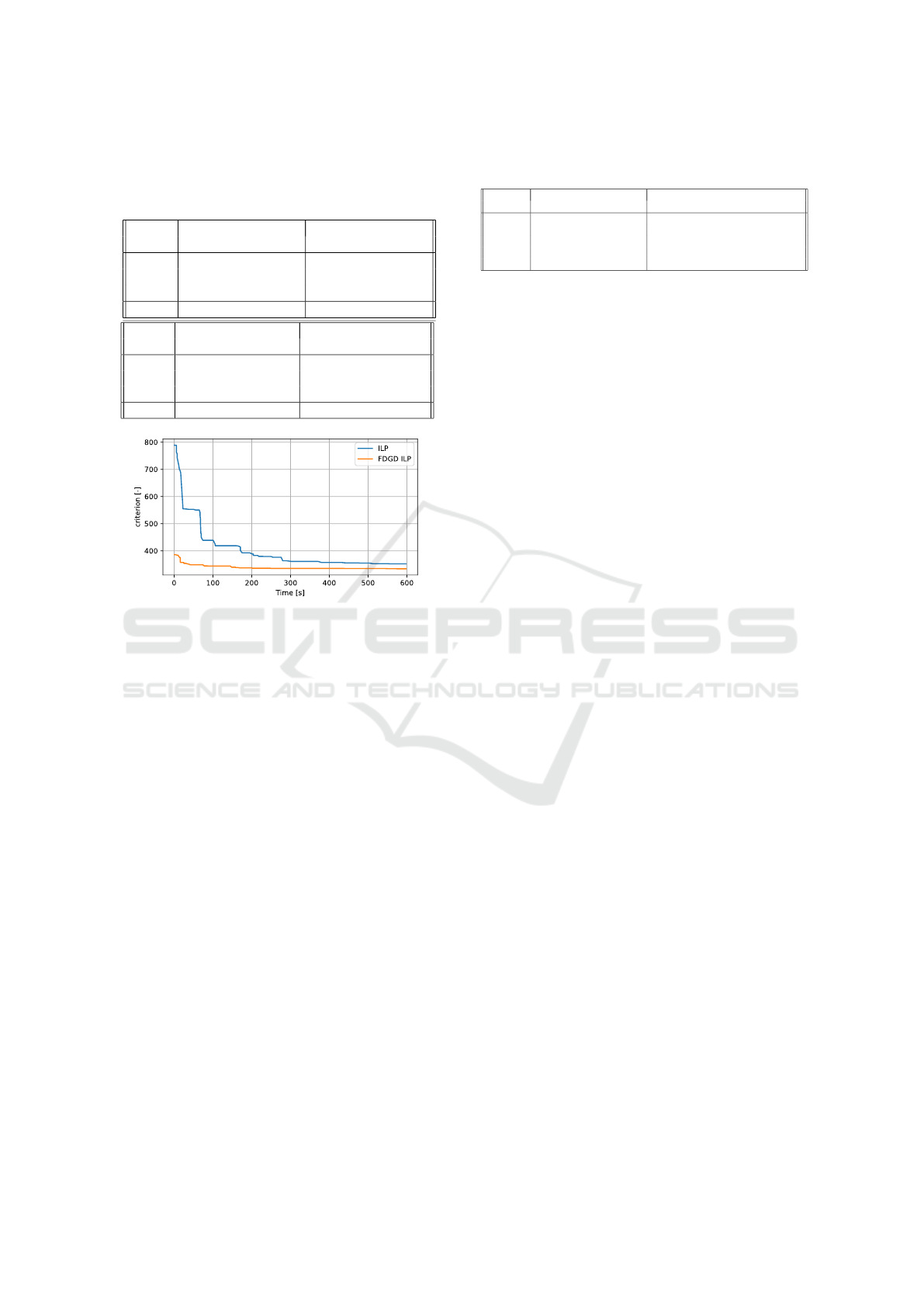
Table 1: Average relative percent gap of method’s criterion

(at given computation time) and best-known result. The

last line shows a number of instances for which the method

achieved a better result than the other one, for sets S

, S

= 0.5 c

= 25

t [s] ILP FDGD ILP ILP FDGD ILP

30 13.36 3.31 45.58 8.50

120 7.23 1.65 21.86 4.51

600 2.75 0.40 7.97 1.28

n = 40 10 30 9 31

= 0.5 c

= 25

t [s] ILP FDGD ILP ILP FDGD ILP

30 81.00 8.02 163.21 9.94

120 35.26 2.84 84.40 3.89

600 12.06 0.00 44.00 0.00

n = 20 0 20 0 20

Figure 4: Example of the changes in criterion value during

computation time.

for both studied weights. The performance gap be-

tween FDGD ILP and stand-alone ILP models in-

creases with larger values of c

and growing instance

size, which makes the FDGD ILP more suitable for

connectivity-oriented and larger problems. We also

found that stand-alone ILP, on average, needs be-

tween 5x to 15x more computation time to ﬁnd the

same-quality solution that FDGD ILP ﬁnds after 30

seconds, depending on an instance size and value of

. A further experiment, which included problem in-

stances from the set S

with 100 independent rectan-

gles, showed that the stand-alone ILP fails to recover

any feasible solution within its 600 s time limit, while

the FDGD ILP’s warm start solution can be extended

to the complete solution almost immediately; making

comparison for set S

unnecessary. Thus, in the rest

of the paper, we only consider FDGD ILP.

5.3 Performance Comparison

To provide an explicit comparison with the state-of-

the-art tools, we used the placer of the open-source

framework ALIGN (Dhar et al., 2021). ALIGN’s an-

notation tool extracted information about grouped el-

ements and symmetries in the design. Test instances

were two Operational Transconductance Ampliﬁers

Table 2: Comparison of proposed FDGD ILP method with

ALIGN placer (Dhar et al., 2021).

ALIGN placer FDGD ILP

instance area [µm

] HPWL [µm] area [µm

] HPWL [µm] time [s]

CC-OTA 73.2 132.2 58.3 141.4 6.0

T-OTA 16.9 28.7 18.6 28.5 0.3

DTS-A 52.8 69.4 44.7 90.0 0.5

SCF 1995.6 478.4 1963.4 485.7 13.8

LE 58.2 47.0 56.5 56.2 6.7

(OTA), a Double Tail Sense Ampliﬁer (DTS-A), a

Switched Capacitor Filter (SCF), and a Linear Equal-

izer (LE). A FinFET 14nm Process design kit (PDK),

part of ALIGN’s repository, was also utilized. Results

containing the area and HPWL of the ﬁnal design both

for ALIGN and our approach FDGD ILP, together

with our solution’s computation time, are shown in

Table 2, with a value of c

tuned for each instance.

Even though our solution was tuned to a slightly

different problem formulation (including the deﬁni-

tion of HPWL with respect to topological structures),

and we needed to manually sanitize the data due to

the differences in input data description, making the

comparison mainly illustrative, our solver found solu-

tions whose evaluation metrics were comparable with

ALIGN’s. This further demonstrates the extensibility

and performance of the FDGD ILP. The computation

time of our ILP solver was limited to approximately

match the computation time of methods presented in a

recent paper (Lin et al., 2022), which were evaluated

on similar instances, to document the relatively short

time our method needed to produce a comparable de-

sign.

5.4 Manual Design Comparison

The industry partner STMicroelectronics provided 17

real-life industrial designs. The BCD technology was

applied, and thus our solution’s capabilities were nec-

essary. Provided designs contained both the input

data (netlist, constraints, and structure list) as well as

the data describing the positions of the devices in the

manual placement created by the experts. Provided

instances contained up to 60 independent rectangles.

The manual and automated placements could be com-

pared with their respective values of L

and L

, and

the placement area. Several runs of the FDGD ILP

were performed, each running for 8 minutes, with

∈ {0.1,15,50}. We have chosen these values to

ﬁnd both the placements prioritizing area and con-

nectivity; however, using even larger values eventu-

ally led to placements that would not be applicable

in the industry setting (unsuitable aspect ratio, exces-

sive empty space). Closest-point L

∗

P2P connectivity

metric was used.

Table 3 contains calculated metrics for each prob-

lem instance, with an average ratio of the automated

Automatic Placer for Analog Circuits Using Integer Linear Programming Warm Started by Graph Drawing

113

Table 3: Values of half perimeter L

in µm, area in µm

and weighted P2P connectivity L

in µm and an average ratio of

placer-produced and manual designs’ metrics aR for real-life instances.

manual placer-produced

= 0.1 c

= 15 c

= 50

instance L

area L

1 158 6118 8572 160 6420 4781 163 6583 4585 172 7347 4595

2 116 2710 1829 88 1911 1193 92 2091 968 96 2247 942

3 106 2650 1336 86 1800 1251 88 1898 448 94 2157 388

4 129 4096 555 112 3107 423 115 3289 285 116 3360 283

5 207 8972 36492 159 6305 13196 170 7013 6078 173 7375 5971

6 178 7698 12756 169 7148 9739 186 8172 6017 197 9013 5852

7 168 6580 14646 162 6558 13677 170 7104 9200 169 7105 8766

8 173 7294 2512 160 6435 2052 169 7082 1740 178 7896 1496

9 243 14129 49076 229 13054 22544 269 18056 17849 254 16151 16543

10 205 10214 41730 192 9192 41542 198 9835 25555 203 10325 24107

11 225 9922 4571 197 9356 1629 200 10000 481 200 10000 481

12 155 5953 5277 133 4440 3105 139 4811 2425 142 5025 2379

13 162 6511 6265 151 5676 5512 157 6161 5055 165 6749 5058

14 247 15235 7676 188 8831 6537 209 10905 2940 209 10872 2625

15 123 3758 1772 115 3286 3698 121 3666 2171 133 3936 2150

16 232 12397 14687 218 11817 7687 229 13037 7524 238 13976 7320

17 247 12525 42532 237 13645 30436 241 14369 26509 262 16474 27778

aR 1.00 1.00 1.00 0.89 0.86 0.78 0.94 0.95 0.53 0.97 1.01 0.51

and manual placement’s metrics:

aR =

∑

i=1

metric

(i)

method

metric

(i)

manual

, (49)

shown in the last row. On average, we may see that all

three placer settings outperformed the manual results

in both optimized metrics L

and L

. Even though

area W ·H is not part of the criterion function, we

were still able to ﬁnd area-wise favorable solutions

in the majority of the cases. Ultimately, for 14 out

of 17 instances, the placer was able to ﬁnd a solu-

tion outperforming manual design in all metrics dis-

cussed in Table 3. Figure 5 demonstrates the differ-

ences between placer-produced solutions, depending

on the value of c

, and includes the distribution of

the devices within topological structures and allowed

pocket merging. Notice the use of differing rectangle

variants in the two designs.

Even though the solver optimized each problem

for up to 480 seconds, we could easily limit the com-

putation time. If the computation was aborted after 60

or 30 seconds, respectively, the found solution would

be worse, on average, by 6 %, or 7 % than the ﬁnal

result. This relatively small gap is made possible due

to the use of FDGD warm start (see Figure 4).

Industry experts validated produced results and

provided qualitative feedback. Experts positively

commend the relatively short time needed to obtain a

high-quality solution; therefore, a solver can be called

several times with different criteria to obtain a port-

folio of solutions, from which experts can easily se-

lect, while hours of work are needed to create a single

Table 4: Average ratio of placer-produced and manual de-

signs’ area and HPWL for real-life instances, depending on

the type of connectivity metric optimized by the solver.

P2P optimizing HPWL optimizing

0.1 15 50 0.1 5

aR 0.89 0.94 0.97 0.88 0.96

area aR 0.86 0.95 1.01 0.83 0.98

HPWL aR 1.08 0.98 0.98 0.92 0.77

placement manually. However, experts pointed out

several suspiciously low values of the P2P connec-

tivity metric of the produced solutions in comparison

with manual designs in Table 3. Thus, we concluded

that the chosen P2P metric does not always capture all

the aspects of the connectivity, and we should focus

on HPWL or minimum spanning tree-based metrics

in the future.

To validate the previous statement, we calculated

the value of HPWL connectivity for each problem in-

stance and each value of c

from Table 3. We also per-

formed a brief experiment with ILP solver optimizing

the HPWL connectivity directly (choosing connectiv-

ity weights suitable for this scenario), and we report

the average ratio of placer-produced and manual de-

sign’s L

, area and HPWL metrics in Table 4.

We can see that in the case of the solver optimiz-

ing the P2P connectivity, the ratio for HPWL is much

worse than its P2P counterpart reported in Table 3.

However, we could still ﬁnd HPWL-wise competitive

designs since the solver found an overall better solu-

tion for 8 instances, making P2P formulation applica-

ble even in this indirect scenario. Furthermore, when

ICORES 2023 - 12th International Conference on Operations Research and Enterprise Systems

114

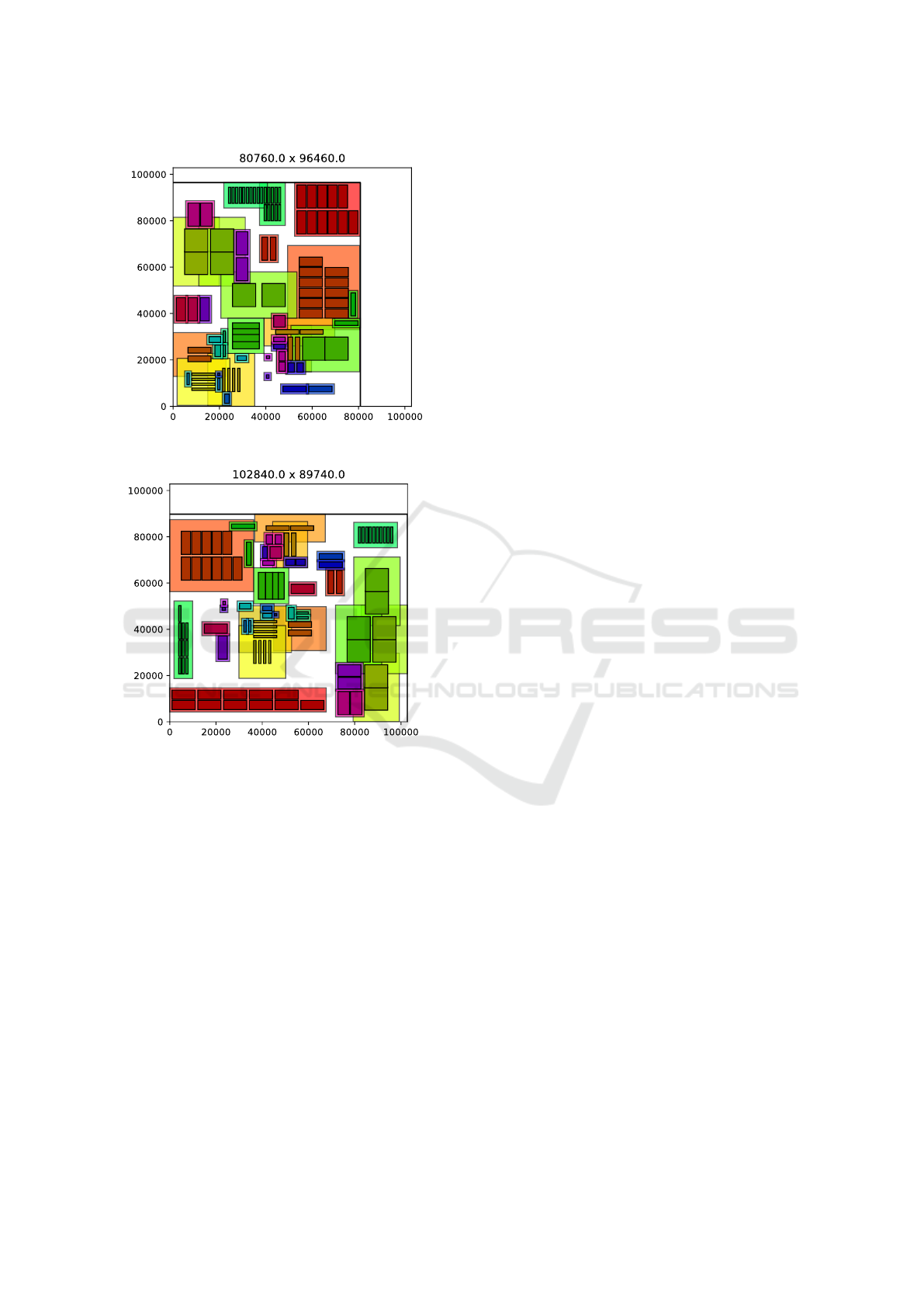
(a) c

= 0.1, area = 7790 µm

(b) c

= 50, area = 9229 µm

Figure 5: Examples of FDGD ILP-produced designs with

different values of c

the solver optimized the HPWL connectivity directly,

we were again able to ﬁnd the solution of overall bet-

ter quality (dominating manual designs in 12 cases),

with an average ratio of HPWL metric equal to 0.92

and 0.77, respectively.

6 CONCLUSION

In this paper, we present the ILP formulation of the

placement process of the physical design of AMS ICs.

We successfully formalized the required constraints

in cooperation with our industry partner STMicro-

electronics to support the BCD technology. We also

provided an FDGD-based warm start heuristic, which

signiﬁcantly improved the performance of the ILP

solver. Ultimately, we evaluated our solution on both

synthetically generated and real-life industrial prob-

lem instances, and we compared our solution with the

open-source ALIGN framework. Both quantitative

results and experts’ feedback regarding the industrial

problem instances showed that our proposed solution

would be beneﬁcial for solving the placement prob-

lem formulated by the industry partner.

Even though our proposed warm start heuristic

signiﬁcantly improves the performance of the ILP

solver, the problem of scalability persists; a number of

decision variables grow quadratically with an increas-

ing number of independent rectangles to be placed.

Therefore, we currently focus on developing a con-

structive heuristic combined with a genetic algorithm

to tackle the placement problem outlined in this paper,

which would not require a state-of-the-art commercial

solver for competitive results. We believe that this ap-

proach, based on methods developed for strip packing

and facility layout problems, could offer competitive

results with the ability to scale.

ACKNOWLEDGMENTS

This work was supported by the Grant Agency of

the Czech Technical University in Prague, grant

No. SGS22/167/OHK3/3T/13.

This work was partially supported by the

EU ICT-48 2020 project TAILOR no. 952215.

REFERENCES

Alvarez-Valdes, R., Parre

no, F., and Tamarit, J. (2008). Re-

active GRASP for the strip-packing problem. Com-

puters & Operations Research, 35(4):1065–1083.

Berger, M., Schr

oder, M., and K

ufer, K.-H. (2009). A

constraint-based approach for the two-dimensional

rectangular packing problem with orthogonal orien-

tations. In Operations Research Proceedings 2008,

pages 427–432. Springer Berlin Heidelberg.

Camm, J. D., Raturi, A. S., and Tsubakitani, S. (1990). Cut-

ting Big M down to Size. Interfaces, 20(5):61–66.

Chen, T.-C., Jiang, Z.-W., et al. (2008). NTUplace3: An an-

alytical placer for large-scale mixed-size designs with

preplaced blocks and density constraints. IEEE Trans-

actions on Computer-Aided Design of Integrated Cir-

cuits and Systems, 27(7):1228–1240.

Coffman, Jr., E. G., Garey, M. R., et al. (1980). Performance

bounds for level-oriented two-dimensional packing al-

gorithms. SIAM Journal on Computing, 9(4):808–

826.

Cohn, J., Garrod, D., et al. (1991). KOAN/ANAGRAM II:

new tools for device-level analog placement and rout-

Automatic Placer for Analog Circuits Using Integer Linear Programming Warm Started by Graph Drawing

115

ing. IEEE Journal of Solid-State Circuits, 26(3):330–

342.

Della Croce, F. and Scatamacchia, R. (2018). Longest pro-

cessing time rule for identical parallel machines revis-

ited. Journal of Scheduling, 23/2:163–176.

Devgan, V., Singh, V., et al. (2019). Using a novel

image analysis metric to calculate similarity of in-

put image and images generated by WAE. In 2019

Amity International Conference on Artiﬁcial Intelli-

gence (AICAI), pages 953–957.

Dhar, T., Kunal, K., et al. (2021). ALIGN: A system for

automating analog layout. IEEE Design and Test of

Computers, 38(2):8–18.

Fruchterman, T. M. J. and Reingold, E. M. (1991). Graph

drawing by force-directed placement. Software: Prac-

tice and Experience, 21(11):1129–1164.

Gurobi Optimization, LLC (2021). Gurobi Optimizer Ref-

erence Manual. https://www.gurobi.com.

Kandu

c, T. and Rodi

c, B. (2015). Optimisation of factory

ﬂoor layout using force-directed graph drawing algo-

rithm. In 2015 38th International Convention on In-

formation and Communication Technology, Electron-

ics and Microelectronics (MIPRO), pages 1087–1092.

Korf, R., Mofﬁtt, M., and Pollack, M. (2010). Optimal

rectangle packing. Annals of Operations Research,

179(1):261–295.

Kubal

ık, J., Kadera, P., et al. (2019). Plant layout optimiza-

tion using evolutionary algorithms. In Industrial Ap-

plications of Holonic and Multi-Agent Systems, pages

173–188, Cham. Springer International Publishing.

Lin, Y., Li, Y., et al. (2022). Are analytical techniques

worthwhile for analog IC placement? In Proceedings

of the 2022 Conference & Exhibition on Design, Au-

tomation & Test in Europe, DATE ’22, page 154–159.

European Design and Automation Association.

Lourenco, N., Vianello, M., et al. (2006). LAYGEN - auto-

matic layout generation of analog ICs from hierarchi-

cal template descriptions. In 2006 Ph.D. Research in

Microelectronics and Electronics, pages 213–216.

Ma, Q., Xiao, L., et al. (2011). Simultaneous handling of

symmetry, common centroid, and general placement

constraints. IEEE Transactions on Computer-Aided

Design of Integrated Circuits and Systems, 30(1):85–

95.

Mallappa, U., Pratty, S., and Brown, D. (2022). RLPlace:

Deep RL guided heuristics for detailed placement op-

timization. In Proceedings of the 2022 Conference &

Exhibition on Design, Automation & Test in Europe,

DATE ’22, page 120–123. European Design and Au-

tomation Association.

Martins, R., Lourenc¸o, N., and Horta, N. (2015). Multi-

objective optimization of analog integrated circuit

placement hierarchy in absolute coordinates. Expert

Systems with Applications, 42(23):9137–9151.

Mirhoseini, A., Goldie, A., et al. (2021). A graph place-

ment methodology for fast chip design. Nature,

594(7862):207–212.

Nesterov, Y. (1983). A method for solving the con-

vex programming problem with convergence rate

o(1/k

). Proceedings of the USSR Academy of Sci-

ences, 269:543–547.

Oliveira, J. F., J

unior, A. N., et al. (2016). A survey on

heuristics for the two-dimensional rectangular strip

packing problem. Pesquisa Operacional, 36:197–226.

Scheible, J. and Lienig, J. (2015). Automation of analog IC

layout: Challenges and solutions. In Proceedings of

the 2015 Symposium on International Symposium on

Physical Design, ISPD ’15, page 33–40.

Spindler, P., Schlichtmann, U., and Johannes, F. M. (2008).

Kraftwerk2—A fast force-directed quadratic place-

ment approach using an accurate net model. IEEE

Transactions on Computer-Aided Design of Integrated

Circuits and Systems, 27(8):1398–1411.

Strasser, M., Eick, M., et al. (2008). Deterministic ana-

log circuit placement using hierarchically bounded

enumeration and enhanced shape functions. In 2008

IEEE/ACM International Conference on Computer-

Aided Design, pages 306–313.

Xie, W. and Sahinidis, N. V. (2008). A branch-and-bound

algorithm for the continuous facility layout problem.

Computers & Chemical Engineering, 32(4):1016–

1028.

Xu, B., Li, S., et al. (2017). Hierarchical and analyti-

cal placement techniques for high-performance ana-

log circuits. In Proceedings of the 2017 ACM on In-

ternational Symposium on Physical Design, ISPD ’17,

page 55–62.

Xu, B., Li, S., et al. (2019a). Device layer-aware analytical

placement for analog circuits. In Proceedings of the

2019 International Symposium on Physical Design,

ISPD ’19, page 19–26.

Xu, B., Zhu, K., et al. (2019b). MAGICAL: Toward

fully automated analog IC layout leveraging human

and machine intelligence: Invited paper. In 2019

IEEE/ACM International Conference on Computer-

Aided Design (ICCAD), pages 1–8.

ICORES 2023 - 12th International Conference on Operations Research and Enterprise Systems

116