Crane Spreader Pose Estimation from a Single View

Maria Pateraki

1,2,3 a

, Panagiotis Sapoutzoglou

1,2 b

and Manolis Lourakis

3 c

School of Rural Surveying and Geoinformatics Engineering, National Technical University of Athens, Greece

Institute of Communication and Computer Systems, National Technical University of Athens, Greece

Institute of Computer Science, Foundation for Research and Technology – Hellas, Greece

Keywords:

Spreader, 6D Pose, Estimation, Single View.

Abstract:

This paper presents a methodology for inferring the full 6D pose of a container crane spreader from a single

image and reports on its application to real-world imagery. A learning-based approach is adopted that starts by

constructing a photorealistically textured 3D model of the spreader. This model is then employed to generate

a set of synthetic images that are used to train a state-of-the-art object detection method. Online operation

establishes image-model correspondences, which are used to infer the spreader’s 6D pose. The performance

of the approach is quantitatively evaluated through extensive experiments conducted with real images.

1 INTRODUCTION

Standard size shipping containers transfer easily be-

tween transport modes and are the single most im-

portant system for the movement of cargo world-

wide (van Ham et al., 2012). Container handling is

fully mechanized and relies predominately on cranes

equipped with spreaders, i.e. lifting devices which

mechanically lock on to containers. Digitization is

currently a trend that is gaining momentum in con-

tainer logistics, aiming to make related processes

more automated, efﬁcient and traceable. Under these

premises, we are interested in monitoring the 6D pose

of a container crane spreader during container load-

ing and unloading operations. Knowledge of the

spreader’s pose can provide input for various uses,

e.g. improve the crane operator’s situational aware-

ness and hence the safety of port workers (Lourakis

and Pateraki, 2022a), ensure that the operator’s driv-

ing commands are within the crane’s safe operating

envelope or perform anti-sway crane control to elimi-

nate undesirable oscillations (Ngo and Hong, 2012).

Numerous visual tracking methods have been de-

veloped and those focusing on 3D tracking (Lepetit

and Fua, 2005; Marchand et al., 2016) can in prin-

ciple facilitate the need for constant monitoring of a

spreader’s pose. However, a serious practical short-

https://orcid.org/0000-0002-8943-4598

https://orcid.org/0000-0001-9885-3981

https://orcid.org/0000-0003-4596-5773

coming of such approaches is that they often are not

concerned with bootstrapping but rather assume that

tracking is initialized by external, typically manual

means. In addition to bootstrapping, periodic initial-

ization is also necessary for recovering from tracking

failures. To address such issues, this work employs

recent results from the object detection and localiza-

tion literature to deal with spreader 6D pose estima-

tion from a single image. To the best of our knowl-

edge, our results are the ﬁrst ones reported dealing

with this particular problem.

The main contributions of our work are: a) the

application of vision techniques to a new domain, b)

a procedure for generating a training dataset based

on systematically rendering a photorealistic object

model from different camera viewpoints, and c) a de-

tailed experimental evaluation of a state-of-the-art ob-

ject detection and localization method (Hoda

n et al.,

2020a) in a real-world setting. The remainder of the

paper is organized as follows. An overview of object

detection and localization approaches is provided in

Section 2. The adopted methodology is presented in

Section 3 and evaluated with the dataset described in

Section 4. The results of the evaluation are presented

in Section 5 and the paper concludes in Section 6.

2 PREVIOUS WORK

Object detection and localization are widely studied

topics in the computer vision community with most

796

Pateraki, M., Sapoutzoglou, P. and Lourakis, M.

Crane Spreader Pose Estimation from a Single View.

DOI: 10.5220/0011788800003417

In Proceedings of the 18th International Joint Conference on Computer Vision, Imaging and Computer Graphics Theory and Applications (VISIGRAPP 2023) - Volume 5: VISAPP, pages

796-805

ISBN: 978-989-758-634-7; ISSN: 2184-4321

 2023 by SCITEPRESS – Science and Technology Publications, Lda. Under CC license (CC BY-NC-ND 4.0)

recent reviews emphasizing the application of deep

learning techniques to both these problems, e.g. (Kim

and Hwang, 2021; He et al., 2021b; Sahin and Kim,

2018; Rahman et al., 2019). The recovery of 6D pose

from a single 2D image is an ill-posed problem due to

the lack of depth. To account for the absence of depth,

researchers rely on exploiting multiple views (Labbe

et al., 2020; Sun et al., 2022), assume geometric pri-

ors (Hu et al., 2022), or use 3D information from dif-

ferent sensors (He et al., 2021b).

In contrast to traditional methods exploiting hand-

crafted features and optimizing classic pipelines, deep

learning methods led to signiﬁcant improvements in

6D object pose estimation in late years (Jiang et al.,

2022). However, a major shortcoming is that these

approaches are extremely data driven and, contrary to

2D vision tasks such as classiﬁcation, object detection

and segmentation, the acquisition of 6D object pose

annotations is much more labor intensive and time

consuming (Hodan et al., 2017; Wang et al., 2020). To

mitigate the lack of real annotations, synthetic images

can be generated via 6D pose sampling and graphics

rendering of a CAD object model. Still, there remains

the concern of this approach performing poorly when

applied to real world images, due to the domain gap

between real and synthetic data (Wang et al., 2020).

Most recent works in object 6D pose estimation

achieve high scores in recall accuracy on benchmark

datasets (He et al., 2021a). However, transferring this

performance to real environments is challenging. Un-

controlled imaging conditions such as dynamic back-

ground, changing illumination, occlusion, etc, that

are often encountered in outdoor environments, fur-

ther aggravate the problem. In the particular case of a

spreader, additional challenges are the large changes

in its appearance and apparent size, cast shadows and

motion blur due to rapid motions and crane vibrations.

Contemporary pose estimation methods based on

the use of deep learning with RGB images have, to

a certain extent, succeeded in effectively handling

objects with weak texture and symmetries. In the

context of the 2020 BOP challenge (Hoda

n et al.,

2020b), several recent approaches were compared

against benchmark datasets that feature objects with

weak texture and symmetries, such as T-LESS (Ho-

dan et al., 2017), LM-O (Brachmann et al., 2014) and

ITODD (Drost et al., 2017). The CosyPose (Labbe

et al., 2020) and EPOS (Hoda

n et al., 2020a) methods

are reported to require 0.5–2 sec processing time per

image, while others exceed 1 min and are therefore

less suitable for near real-time applications. Apart

from being computationally efﬁcient, EPOS effec-

tively manages global and partial object symmetries,

therefore it was selected as the basis of spreader pose

estimation in this work.

3 METHODOLOGY

3.1 Overview

Training a neural model for the detection and 6D

pose estimation of a spreader requires the collec-

tion of a large number of training images that de-

pict the spreader from various vantage points. Ow-

ing to the spreader’s large physical dimensions and

the practical difﬁculties of thoroughly imaging it un-

der controlled conditions for recovering the ground

truth poses, amassing an adequate training dataset is

far from being a trivial task. To overcome this, it

was decided to employ synthetic images for training,

hence a photorealistic textured model of the spreader

was constructed ﬁrst. Then, the training dataset was

generated by systematically rendering images of the

textured spreader model from different camera view-

points which densely sample the 6D pose space.

Equipped with a trained model, online inferencing

with EPOS permits the recovery of the 6D spreader

pose. More details are provided in the subsections

that follow.

3.2 Object Pose Estimation

The EPOS method (Hoda

n et al., 2020a) relies pri-

marily on RGB images while additional depth infor-

mation may be exploited to improve the accuracy of

the required rendering of object models. Objects are

represented via sets of compact surface regions called

fragments, which are used to handle symmetries by

predicting multiple potential 2D-3D correspondences

at each pixel. EPOS establishes 2D-3D correspon-

dences by linking pixels with predicted 3D locations

and then a Perspective-n-Point (PnP) algorithm em-

bedded in a RANSAC (Fischler and Bolles, 1981)

framework is used to estimate the 6D pose.

Initially, a regressor associates each of the sur-

face fragments of the object to predict the correspond-

ing 3D location expressed in 3D fragment coordi-

nates. Then, a single deep convolutional neural net-

work (CNN) with a DeepLabv3+ (Chen et al., 2018)

encoder-decoder is adopted to densely predict a) the

probability of each object’s presence, b) the proba-

bility of the fragments given the object’s presence,

and c) the precise 3D location on each fragment in

3D fragment coordinates. For training the network, a

per-pixel annotation in the form of an object label, a

fragment label, and 3D fragment coordinates are pro-

vided. Hypotheses are next formed by a locally op-

Crane Spreader Pose Estimation from a Single View

797

timized RANSAC variant (Barath and Matas, 2018)

and pose is estimated by the P3P solver of (Kneip

et al., 2011). Finally, pose is reﬁned from all inliers

using the EPnP solver (Lepetit et al., 2009) followed

by non-linear minimization of the reprojection error.

3.3 Pose Error Metrics

To assess the error pertaining to the pose estimated

for an image frame, different metrics are employed.

The ﬁrst set of metrics quantiﬁes the absolute angu-

lar and positional errors with respect to the ground

truth. More speciﬁcally, given the true camera ro-

tation R

and translation t

, the error for an esti-

mated rotation R

is the angle of rotation about a

unit vector that transfers R

to R

, computed as

arccos((trace(R

) − 1)/2) (Huynh, 2009). The

absolute error for an estimated translation t

is the

magnitude of the difference of the translation parts,

i.e. ||t

− t

|| with the vertical bars denoting the vec-

tor norm. The second set of metrics are the relative

angular and positional errors as employed by (Lep-

etit et al., 2009). These are respectively calculated

as ||q

− q



||q

||, where q

and q

are the unit

quaternions corresponding to the rotation matrices,

while the relative error of an estimate t

is given by

||t

− t



||t

||.

Further to these metrics, we also used the aver-

age distance for distinguishable (ADD) objects (Hin-

terstoisser et al., 2012), which quantiﬁes the aver-

age misalignment between the model’s vertices in the

true and estimated pose by calculating the average

distance between corresponding mesh model vertices

transformed by the ground truth and the estimated

pose. More concretely, for a mesh model with N ver-

tices x

, the ADD alignment error is given by

E =

∑

i=1

∥(R

+ t

) − (R

+ t

)∥, (1)

where {R

, t

} is again the true pose and {R

, t

}

the estimated one. The ﬁrst and second set of metrics

consider the angular and positional errors separately,

whereas the ADD indirectly accounts for both pose

components simultaneously.

3.4 Object Model Texturing

Application of EPOS requires high ﬁdelity textured

3D models of the objects of interest to be avail-

able. In the case of the crane spreader, a texture-

less mesh model was initially designed with the aid

of CAD software, using actual physical dimensions

obtained from engineering diagrams. The opening of

the telescopic beams of the spreader model was cho-

sen to match that of a 40 ft container. The model has

medium level detail and consists of 724 faces and 332

vertices. More detailed models were avoided as they

do not noticeably improve the accuracy of pose es-

timation, while incurring a larger computational cost

to be rendered. To construct a photorealistic textured

model, a set of images were collected with a handheld

commodity camera from different viewpoints around

the spreader and combined together with its CAD

mesh model for texture mapping.

Based on freely available software tools, two dif-

ferent texturing approaches were tested. The ﬁrst em-

ployed the MeshLab

open source software and its in-

tegrated workﬂow for texture mapping. The standard

approach for texturing a model’s polygons is to ex-

tract the texture from the image whose camera optical

axis is as close to being parallel to a certain face nor-

mal as possible. Although the camera position of the

images was correctly estimated from manual raster

alignment in MeshLab, in some cases the texture was

taken from images for which the angle between the

camera axis and the surface normal was not the small-

est, resulting in perspective distortions. Further in-

vestigation into this issue revealed that MeshLab gen-

erally assumes that the input geometric models con-

sist of dense meshes, for which such perspective er-

rors are barely visible. However, this texture mapping

workﬂow is less suited to CAD models with sizeable

triangular faces as is the case with the spreader model.

The second approach was based on Blender

which has certain provisions for automatically pro-

jecting images to meshes, though it assumes sim-

ple geometric shapes. For the spreader, a manual

texture mapping process was followed, summarized

as follows. First, the model’s origin and axes were

transformed to conform to the input conventions of

the training data later used by EPOS for object pose

inference. Then, a UV texture map was generated

automatically in Blender unfolding the model faces

based on edges characterized as “sharp”, i.e. edges

formed by two adjacent faces with an angle between

their normals exceeding a threshold value. For cer-

tain faces that Blender erroneously marked as being

non-coplanar, despite their normals exhibiting negli-

gible differences, a postprocessing step was carried

out on the mesh model. Speciﬁcally, a plane was ﬁt-

ted to selected points to assess whether large errors

were present and then the mesh was re-triangulated

generating coplanar faces. For a few self-occluded

parts of the spreader that did not appear in any im-

age, texture was sampled from nearby image areas to

https://www.meshlab.net

https://www.blender.org

VISAPP 2023 - 18th International Conference on Computer Vision Theory and Applications

798

Figure 1: The crane spreader (left), and renderings of its

mesh (middle) and ﬁnal textured models (right). For sim-

plicity, the three moving gather guides at each end beam of

the spreader have not been modeled.

ﬁll the remaining empty regions. Sample views of the

mesh model and the ﬁnal textured model are in Fig. 1.

3.5 Image Rendering

For rendering the training dataset (see Sec. 3.6), a

custom renderer based on OpenGL’s shader pipeline

was developed. This renderer encompasses different

shaders to perform wireframe, textured and depth ren-

dering. Speciﬁcally, for depth map generation, depth

was computed using a depth shader that transforms

the vertex coordinates of the model to the viewspace

of the camera. The depth value was then obtained by

negating the z component of the resulting points.

In addition to the aforementioned rendering pro-

cedure, an algorithm for hidden lines removal based

on z-buffering was developed that proved very useful

for the visual assessment of the estimated poses on the

test sequences (see Sec. 5). Hidden lines removal is

closely associated with the wireframe display mode

and is used to suppress the rendering of edges that

are occluded from a certain camera perspective. Ad-

ditionally, it discards nominal edges (i.e. edges/lines

that separate faces which are coplanar and thus be-

long to the same plane). To discard edges occluded

from the camera viewpoint, the algorithm uses the

depth buffer to store the depth of each fragment of the

model when rendered and performs a depth test with a

depth mask of the scene rendered with lines. Further-

more, the nominal edges are excluded by computing

the normals cross product for every pair of adjacent

faces. If the cross product is close to zero, the edge

is discarded as being nominal (e.g. a subdivision of a

quad face into two triangles).

3.6 Training Dataset

Training data were generated by systematically ren-

dering the textured spreader model against a black

background from different camera viewpoints, thus

densely sampling different 6D poses of the spreader.

With the spreader model placed at the center of a half

sphere and the use of spherical coordinates φ and θ,

different images were rendered at camera positions

around hemispheres of radial distances ranging from

10 to 30 meters with a step of 5 meters (see Fig. 2).

Figure 2: The spherical coordinate system employed in

sampling the 6D space of spreader poses for training.

The azimuthal angle φ was set in the range of 0-360

degrees whereas the polar angle θ in the range of 0-90

degrees. For both angles, the step interval for render-

ing different viewpoints was set to 5 degrees. Val-

ues of θ exceeding 90 degrees were not considered

as bottom views of the spreader are not encountered

in reality and hence were excluded from the training

dataset. A total of 6840 images were generated. In-

dicative thumbnails of rendered views at a distance of

10 m from the spreader’s centroid are shown in Fig. 3.

The rendered images used for training were

720×540 pixels as that was the largest size that could

be accommodated in the memory available on the

particular GPU card used in the experiments (i.e.

NVIDIA GeForce RTX 3060). 75% of the rendered

dataset, i.e. 5130 images, were randomly selected

for training, whereas the remaining 25% (i.e. 1710

images) were used for validation. Hyperparameters

were tuned based on a number of experiments opti-

mizing in parallel the training loss. The base learn-

ing rate was set to 3 × 10

−5

and a polynomial decay

learning rate schedule was used with power equal to

0.7, while the number of training steps was 2 × 10

Results on the training loss are shown in Fig. 4. The

total loss and the training loss for visible object classi-

ﬁcation are shown in the top left and top right, while

in the bottom left and bottom right are the training

loss for visible fragments and the fragment localiza-

tion loss. For the latter, regression is used for estimat-

ing the 3D coordinates of the fragments. In all four

cases, the total loss has gradually reduced and ﬁnally

stabilized.

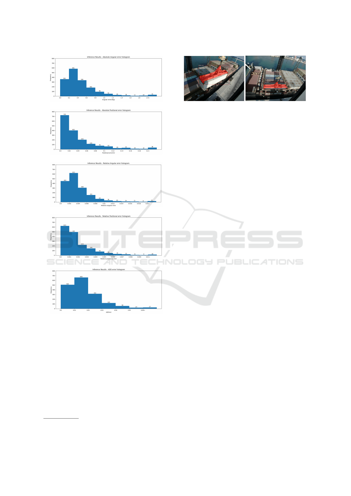
Figure 5 shows sample qualitative results on the

validation data regarding the predicted poses. The

error metrics illustrated in Fig. 6 depict the distri-

bution of the absolute angular and positional errors.

In addition, the distributions of the relative angular

and positional errors, as well as the ADD errors are

also shown. To account for rotational symmetry in

Crane Spreader Pose Estimation from a Single View

799

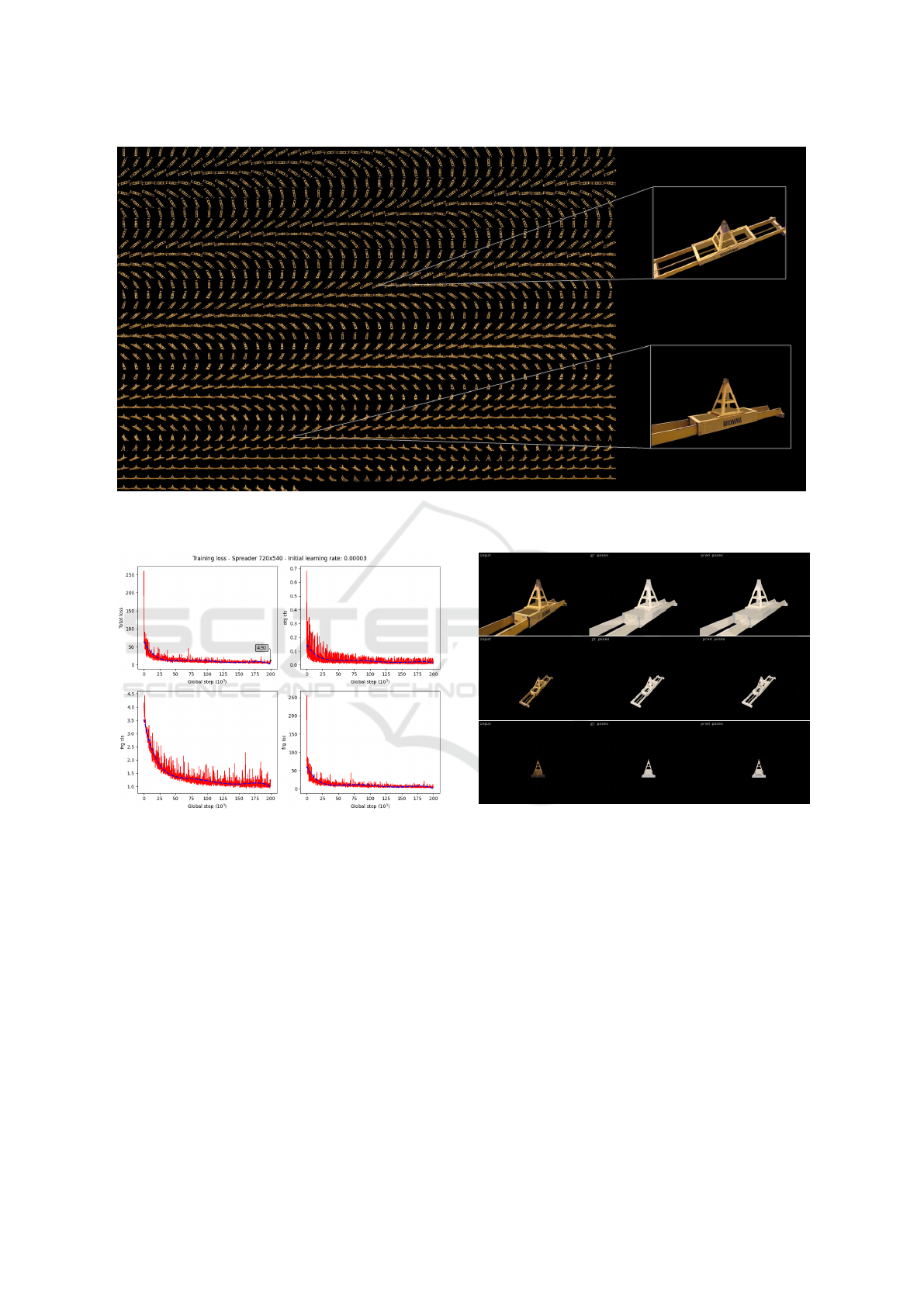
Figure 3: Sample rendered images of the spreader model around a hemisphere of radius of 10 m, with an azimuthal angle φ

range of [0

◦

− 360

◦

] and polar angle θ range of [0

◦

− 90

◦

] with an increment of 5

◦

Figure 4: Total loss and number of steps (top left), training

loss for visible object classiﬁcation (top right), training loss

for visible fragments (bottom left) and fragment localiza-

tion loss (bottom right).

the vertical (i.e., z) axis of the spreader, the errors for

both the estimated and the ﬂipped pose (i.e., rotated

by π around the z-axis) were considered and the pose

yielding the smallest of the two was used in the calcu-

lation of the ﬁnal errors. The absolute angular errors

are in general below 1

◦

and the absolute positional er-

rors below 0.1 m. The relative angular and positional

errors are below 0.01 in both cases, whereas the ADD

error is in most cases below 0.04 m.

Figure 5: Example image results on validation data.

Input image (left), ground truth pose (middle), re-

gressed/predicted pose (right).

3.7 Background Removal

Preliminary tests with real images indicated that back-

ground clutter present in them often gave rise to erro-

neous poses, thus it was decided to perform a 2D seg-

mentation of the spreader before inference. In order

to eliminate the background, a model was trained to

automatically detect the region corresponding to the

spreader’s image and then use it as a 2D mask for per-

forming pose inference.

The dataset for training the mask detector com-

prised of a number of annotated frames for training

and validation. A total of 224 frames (188 training

VISAPP 2023 - 18th International Conference on Computer Vision Theory and Applications

800

(a)

(b)

(c)

(d)

(e)

Figure 6: Results on validation data (1710 images). (a)

absolute angular errors, (b) absolute positional errors, (c)

relative angular errors, (d) relative positional errors and (e)

mean misalignment errors (ADD).

and 36 validation) with sufﬁcient diversity in spreader

poses, and originating from ﬁve different video se-

quences acquired in the port environment were man-

ually annotated using the VGG Image Annotator

. In

order for the dataset to ﬁt in the available GPU mem-

ory, its image frames were resampled to 1024×768

while maintaining their original aspect ratio.

Initially, we experimented with the Tensorﬂow-

based implementation of the Mask R-CNN algo-

https://www.robots.ox.ac.uk/

∼

vgg/software/via/

Figure 7: Results on 2D segmentation with the Mask R-

CNN algorithm. The inaccuracies of the detected mask

boundaries are clearly visible in the left image.

rithm (He et al., 2017). The inference results were

mostly accurate but in certain frames the spreader

was not segmented correctly, with the segmentation

masks also exhibiting a wave effect at their bound-

aries, as shown in Fig. 7. In an effort to alleviate these

problems, we used the Detectron2 library (Wu et al.,

2019), which in addition attains shorter training times

due to the PyTorch-based implementation of Mask R-

CNN.

4 REAL IMAGES AND GROUND

TRUTH POSES

The images we employed for evaluation originate

from our publicly available dataset which depicts a

moving crane spreader while unloading a container

cargo vessel (Lourakis and Pateraki, 2022b). The

dataset consists of several image sequences contain-

ing segments with the spreader being vacant and car-

rying a container. All image sequences were acquired

from a viewpoint similar to that of the crane oper-

ator using a camera installed next to the operator’s

cabin at a height of approximately 20 meters above

the quay. Owing to this setup, the camera moves with

the crane, giving rise to a non-stationary image back-

ground. This further induces large variability in illu-

mination within each image sequence and across the

image sequences comprising the dataset, as the se-

quences were captured outdoors at different times of

the day.

For every image frame, the dataset includes the

corresponding ground truth pose of the spreader. Ac-

quiring ground truth poses for real world sequences

entails certain manual effort and is a rather arduous

task. Before proceeding to the presentation of re-

sults, it is important to describe how were the ground

truth poses for the dataset obtained since the proce-

dure adopted impacts their accuracy.

Initially, the following options were considered

for the spreader and were both deemed inapplica-

ble. Non-visual sensors, e.g. RTK GNSS re-

ceivers (Lourakis et al., 2020) could not be de-

Crane Spreader Pose Estimation from a Single View

801

ployed due to installation limitations and the fact

that their measurements would be adversely affected

by interference caused by the crane’s metallic struc-

ture. Another choice would be the installation of

visual ﬁducial markers (Garrido-Jurado et al., 2014)

on the spreader, however this would affect its ap-

pearance and consequently potentially interfere with

the pose estimation process. Alternatively, ground

truth poses were obtained with the following semi-

automatic procedure. The spreader’s pose in a cer-

tain image frame was estimated by ﬁrst delineat-

ing in that image a few characteristic line segments

whose pre-images in the spreader’s mesh model were

easily identiﬁable and then using them to estimate

a preliminary spreader pose with a Perspective-n-

Line (PnL) solver (Wang et al., 2019) embedded in

RANSAC (Fischler and Bolles, 1981) for safeguard-

ing against outliers. Finally, the preliminary pose es-

timate was reﬁned with non-linear least squares by

minimizing the re-projection error between the ac-

tual image line segments and their predicted locations

with Levenberg-Marquardt (Lourakis, 2004).

To obtain the spreader’s poses for an entire video

sequence, the pose in the ﬁrst frame of the sequence

was estimated with the procedure outlined in the pre-

vious paragraph, using a few model-to-image cor-

respondences that were speciﬁed manually. This

ﬁrst-frame pose was used to initialize our tracker

from (Lourakis and Pateraki, 2021) and the spreader

was tracked until the model of the spreader rendered

on images with the estimated pose began to visually

deviate from its true image. At the underlying frame,

the pose was again estimated interactively with PnL

and Levenberg-Marquardt reﬁnement, the tracker was

re-initialized with it and the process was repeated as

many times as necessary for the remaining frames.

In this manner, the pose was estimated interactively

at certain intermediate keyframes (typically up to a

handful for each sequence) and then propagated by

frame-to-frame tracking between them. This proce-

dure enabled the collection of ground truth poses with

limited manual intervention in a reasonable amount of

time. The trade-off is that the data obtained are actu-

ally pseudo ground truth.

5 EVALUATION RESULTS

This section provides quantitative experimental re-

sults regarding the accuracy of the single-view pose

estimator using images captured in a real port en-

vironment as discussed in Section 4. In addition

to pose accuracy, computational performance on two

low-cost GPU models is also assessed. The employed

images have a resolution of 1928×1448 pixels. Prior

to further processing, images were undistorted and

subsampled to a lower resolution, maintaining their

aspect ratio. In the reported experiments, eight im-

age sequences were used, each being several hundred

frames long and with a total number of around 7000

image frames.

The background of each input image was seg-

mented out as described in Section 3.7. After seg-

mentation, the 2D mask of the foreground (i.e., pre-

sumably the spreader) was scaled to match the im-

age size of the inference images used in the test se-

quences (1024×768 and 720×570). Additionally, a

rigid transformation was applied to compensate for

the different axes and coordinate origin conventions

employed in EPOS. Speciﬁcally, EPOS requires the

model’s origin to be on the center of its 3D bounding

box, and the z axis to point upward. The model was

trained with the spreader being centered in images,

whereas in the test image sequences the spreader may

appear in different locations near the periphery of an

image. Therefore, before running the estimator, each

masked image was warped to a new one by applying a

homography transforming the center of the spreader’s

bounding box to the image principal point. This ho-

mography has the effect of rotating the ray corre-

sponding to the bounding box center so as to make

it coincide with the camera principal axis. The under-

lying rotation matrix was also used to transform the

ground truth poses so that the spreader is centered in

the new images. The ﬁnal pre-processing step regards

adjusting the camera intrinsic parameters according to

the image size used for the inference, while maintain-

ing a constant aspect ratio. The transformed ground

truth poses used in the inference were computed as

[R | t]

= R

· [R | t]



0 1





I t

0 1



, (2)

where [R | t]

is the transformed ground truth pose

(according to EPOS conventions), R

is the rotation

matrix centering the spreader, R

is the rotation for

the y-z axis swap and t

is the transformation to set

the origin to the spreader’s 3D bounding box.

The trained model for pose estimation was ini-

tially assessed on two sequences with different image

resolutions, namely 1024×768 and 720×540 pixels,

to investigate the relation of image resolution with the

6D pose errors and the inference times. The experi-

ments conﬁrmed that the inference time was reduced

using images with resolution 720×540 pixels without

signiﬁcantly increasing the pose error metrics. The

main reason is that the images used for training were

720×540 pixels in size. Yet, in both cases accuracy

dropped for distant views of the spreader as in such

VISAPP 2023 - 18th International Conference on Computer Vision Theory and Applications

802

Figure 8: Indicative results from the test sequences with the

predicted pose and the visible rendered model edges super-

imposed in white (best viewed zoomed in).

situations the spreader is imaged in a small number of

pixels.

Indicative image results are shown in Fig. 8, where

the ADD, absolute angular and absolute translational

errors are reported. For a qualitative visual assess-

ment, the visible wireframe lines of the model are ren-

dered superimposed on the input images. A correctly

estimated pose should give rise to an overlaid model

that aligns well with the contours and surfaces of the

actual spreader in an image. Figure 9 illustrates the

mean ADD error obtained for each image sequence of

the dataset, whereas Fig. 10 depicts the distribution of

ADD errors for the two image sequences comprised

of the largest number of frames. For the most part,

the mean misalignment error is less than 0.7 m and in

the majority of the sequences below 0.3 m. Further-

more, the distribution of the errors in two indicative

sequences with approximately 1300 frames each in-

dicates that errors tend to be less than 0.2 m. We note

at this point that the literature often considers a pose

to be correct if its ADD is below a threshold chosen as

the 10% of the object diameter (Hinterstoisser et al.,

2012), which for the 12.44 m of the spreader equals

1.244 m. Table 1 summarizes for each sequence the

minimum, mean and maximum ﬁgures for the ADD,

absolute angular and positional error.

The mean absolute angular errors are in general

below 5

◦

except for one sequence (i.e., 095324), in

which the mean absolute angular error increases to

around 8

◦

. It has been further observed that errors

tend to be about 2

◦

− 3

◦

and for distant views the er-

rors may increase up to 5

◦

− 6

◦

. For the same se-

quences, the mean absolute positional errors are about

0.5 m − 0.6 m and for far away views less than 3.5

m. It is to be noted that the larger errors in one se-

quence are partially attributed to erroneous segmen-

tation in cases of nearby objects having similar color

distributions with these of the spreader and partly to

inaccurate ground truth poses. To mitigate the effect

of the latter, it was decided to exclude images yield-

ing highly erroneous poses from further considera-

tion in the computation of the error statistics. Thus,

90% of the frames with smaller ADD errors were re-

tained, discarding the remaining 10%. The choice of

the ADD instead of the absolute angular or positional

error for selecting these frames is justiﬁed by the fact

that we are mostly interested in the misalignment of

the spreader at the estimated pose with respect to its

ground truth conﬁguration rather in the magnitude of

the angular or positional error. An additional argu-

ment in favor of a surface alignment metric is that for

elongated objects like the spreader, a small deviation

in rotation can still result in a substantial misalign-

ment of the object surface. The results in Table 1 fol-

low the above arrangement, keeping poses within the

90th percentile with respect to their ADD error and

computing for these the ADD as well as the absolute

angular and positional error statistics.

Figure 11 illustrates an indicative comparison of

inference times for two different GPU models (specif-

ically the GeForce RTX 3060 & RTX 3070) employed

with two sequences for the 720×540 image resolu-

tion. These tests aim to quantify the impact the se-

lection of an affordable GPU has on inference times.

The RTX 3060 is equipped with 12GB of GDDR6

memory, which is considerably larger compared to the

8GB memory offered by the RTX 3070. However,

since inferencing is a compute-bound operation and

the RTX 3070 has a higher number of CUDA cores

(5888) compared to those in the RTX 3060 (3584

cores), it achieves shorter processing times.

Overall, these ﬁndings attest that the proposed

methodology can support the initialization or the re-

initialization of our model-based tracker (Lourakis

and Pateraki, 2021) with an approximate pose of

reasonable accuracy. The tracker can thus be aug-

mented by the presented pose estimator running in

a parallel thread and providing an additional cue

for pose estimation when necessary. On the other

hand, the estimator is not fast enough for tracking-

by-detection (Lepetit and Fua, 2005) in real-time.

6 CONCLUSION

Capitalizing on recent developments in object de-

tection and localization, this paper has presented a

methodology for spreader 6D pose estimation from

a single image. It starts by constructing a photo-

realistic textured mesh model of the spreader which

is subsequently systematically rendered from differ-

ent camera viewpoints to generate a training dataset

augmented with the employed poses. Pose inference

with EPOS (Hoda

n et al., 2020a) yields a pose esti-

Crane Spreader Pose Estimation from a Single View

803

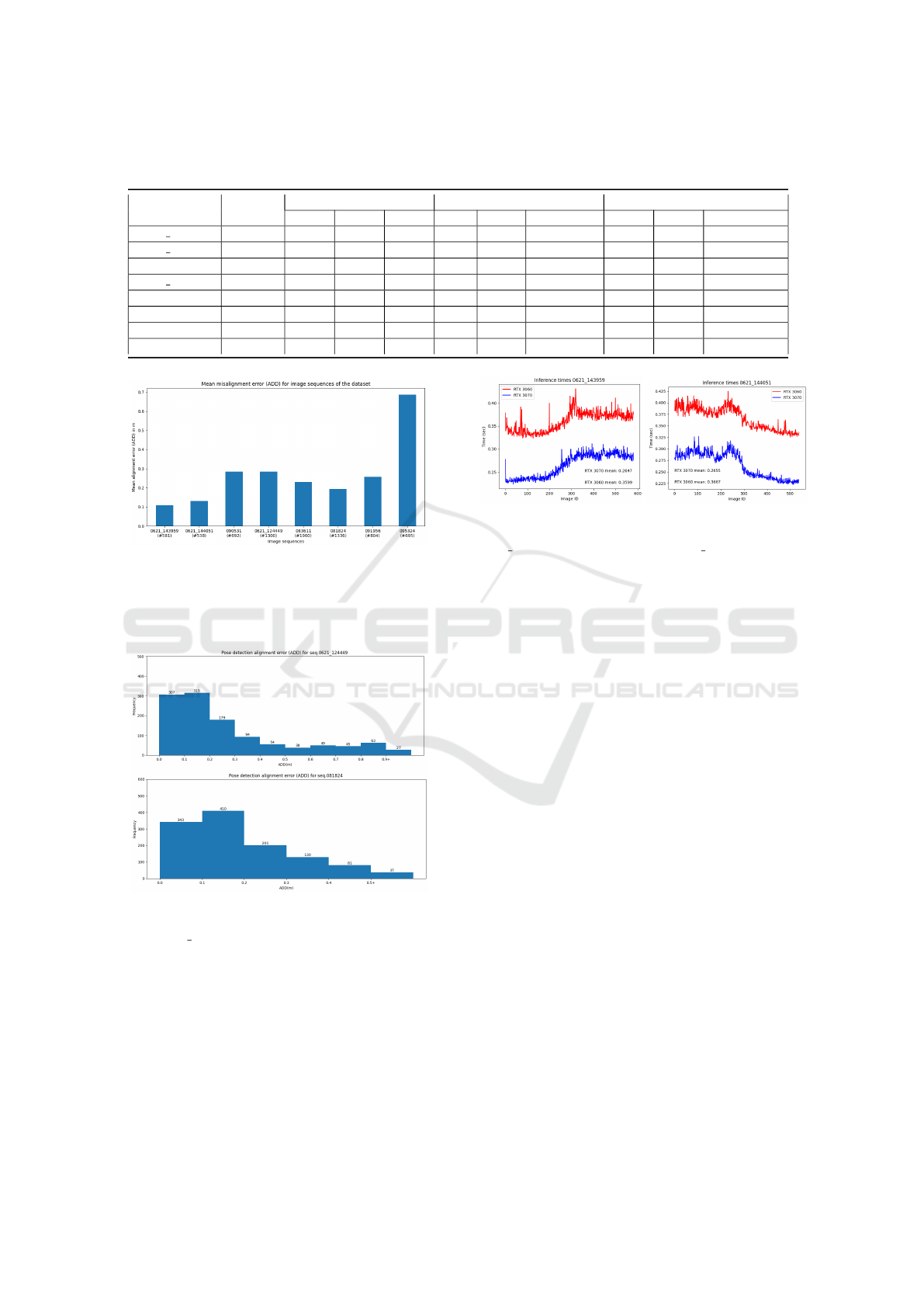
Table 1: Quantitative results for each test sequence and corresponding image sizes. The minimum, maximum and mean values

are shown for ADD, absolute angular and positional errors.

Sequence #frames

ADD error (m) Absolute Angular Error (

◦

) Absolute Positional Error (m)

min mean max min mean max min mean max

0621 144051 538 0.012 0.131 0.359 0.11 1.81 5.79 0.028 0.309 1.917

0621 143959 581 0.015 0.109 0.230 0.06 1.50 4.57 0.008 0.273 1.256

090531 692 0.026 0.284 0.613 0.42 3.65 10.48 0.036 0.570 3.873

0621 124449 1300 0.012 0.284 0.949 0.25 4.66 19.15 0.017 0.934 4.761

083611 1060 0.029 0.230 0.642 0.17 4.35 11.77 0.034 0.535 3.525

081824 1336 0.016 0.194 0.563 0.11 1.87 6.65 0.018 0.641 3.028

091956 804 0.037 0.257 0.700 0.15 3.36 10.74 0.025 0.650 3.116

095324 695 0.08 0.686 1.286 0.47 7.93 16.36 0.029 0.905 2.389

Figure 9: Mean misalignment error (ADD) for all eight im-

age sequences. In the horizontal axis, the names of the se-

quences from the dataset are shown along with their corre-

sponding #number of frames in parentheses. The vertical

axis shows the mean ADD in meters (m).

Figure 10: Distribution of the misalignment error (ADD)

for two indicative image sequences, speciﬁcally image se-

quence 0621 12449 with 1300 frames (top) and sequence

81824 with 1336 frames (bottom).

mate that can complement recursive 3D tracking ap-

proaches such as (Lourakis and Pateraki, 2021) for

bootstrapping and re-initialization. Comprehensive

experiments performed with real-world images anno-

tated with spreader poses have demonstrated the efﬁ-

cacy of the approach.

Figure 11: Inference times per image frame for two se-

quences using two different GPUs. Timings from sequence

0621 143959 (left) and sequence 0621 144051 (right) are

shown. For both sequences, images of 720×540 pixels were

used.

ACKNOWLEDGEMENTS

This work has received funding from the EU Horizon

2020 programme under GA No. 101017151 FELICE.

REFERENCES

Barath, D. and Matas, J. (2018). Graph-cut RANSAC. In

Proceedings of the IEEE conference on computer vi-

sion and pattern recognition, pages 6733–6741.

Brachmann, E., Krull, A., Michel, F., Gumhold, S., Shot-

ton, J., and Rother, C. (2014). Learning 6D object

pose estimation using 3D object coordinates. In Euro-

pean conference on computer vision, pages 536–551.

Springer.

Chen, L.-C., Zhu, Y., Papandreou, G., Schroff, F., and

Adam, H. (2018). Encoder-decoder with atrous sepa-

rable convolution for semantic image segmentation. In

Proceedings of the European conference on computer

vision (ECCV), pages 801–818.

Drost, B., Ulrich, M., Bergmann, P., Hartinger, P., and

Steger, C. (2017). Introducing MVTec ITODD –

A dataset for 3D object recognition in industry. In

Proceedings of the IEEE international conference on

computer vision workshops, pages 2200–2208.

Fischler, M. and Bolles, R. (1981). Random sample consen-

sus: A paradigm for model ﬁtting with applications to

image analysis and automated cartography. Commun.

ACM, 24(6):381–395.

VISAPP 2023 - 18th International Conference on Computer Vision Theory and Applications

804

Garrido-Jurado, S., Mu

noz Salinas, R., Madrid-Cuevas, F.,

and Mar

ın-Jim

enez, M. (2014). Automatic generation

and detection of highly reliable ﬁducial markers under

occlusion. Pattern Recognition, 47(6):2280–2292.

He, K., Gkioxari, G., Doll

ar, P., and Girshick, R. (2017).

Mask R-CNN. In IEEE International Conference on

Computer Vision (ICCV), pages 2980–2988.

He, Y., Huang, H., Fan, H., Chen, Q., and Sun, J. (2021a).

FFB6D: A full ﬂow bidirectional fusion network for

6D pose estimation. In Proceedings of the IEEE/CVF

Conference on Computer Vision and Pattern Recogni-

tion, pages 3003–3013.

He, Z., Feng, W., Zhao, X., and Lv, Y. (2021b). 6D pose

estimation of objects: Recent technologies and chal-

lenges. Applied Sciences, 11(1):228.

Hinterstoisser, S., Lepetit, V., Ilic, S., Holzer, S., Bradski,

G., Konolige, K., and Navab, N. (2012). Model based

training, detection and pose estimation of texture-less

3D objects in heavily cluttered scenes. In Asian Conf.

on Computer Vision, pages 548–562. Springer.

Hoda

n, T., Bar

ath, D., and Matas, J. (2020a). EPOS: Es-

timating 6D pose of objects with symmetries. IEEE

Conference on Computer Vision and Pattern Recogni-

tion (CVPR).

Hodan, T., Haluza, P., Obdr

alek,

S., Matas, J., Lourakis,

M., and Zabulis, X. (2017). T-LESS: An RGB-D

dataset for 6D pose estimation of texture-less objects.

In 2017 IEEE Winter Conference on Applications of

Computer Vision (WACV), pages 880–888. IEEE.

Hoda

n, T., Sundermeyer, M., Drost, B., Labb

e, Y., Brach-

mann, E., Michel, F., Rother, C., and Matas, J.

(2020b). BOP challenge 2020 on 6D object localiza-

tion. In European Conference on Computer Vision,

pages 577–594. Springer.

Hu, H., Zhu, M., Li, M., and Chan, K.-L. (2022). Deep

learning-based monocular 3D object detection with

reﬁnement of depth information. Sensors, 22(7).

Huynh, D. Q. (2009). Metrics for 3D rotations: Comparison

and analysis. J. Math. Imaging Vis., 35(2):155–164.

Jiang, X., Li, D., Chen, H., Zheng, Y., Zhao, R., and Wu,

L. (2022). Uni6D: A uniﬁed CNN framework without

projection breakdown for 6D pose estimation. In Pro-

ceedings of the IEEE/CVF Conference on Computer

Vision and Pattern Recognition, pages 11174–11184.

Kim, S.-h. and Hwang, Y. (2021). A survey on deep learn-

ing based methods and datasets for monocular 3D ob-

ject detection. Electronics, 10(4):517.

Kneip, L., Scaramuzza, D., and Siegwart, R. (2011). A

novel parametrization of the perspective-three-point

problem for a direct computation of absolute camera

position and orientation. In CVPR 2011, pages 2969–

2976. IEEE.

Labbe, Y., Carpentier, J., Aubry, M., and Sivic, J. (2020).

CosyPose: Consistent multi-view multi-object 6D

pose estimation. In Proceedings of the European Con-

ference on Computer Vision (ECCV).

Lepetit, V. and Fua, P. (2005). Monocular model-based 3D

tracking of rigid objects: A survey. Foundations and

Trends in Computer Graphics and Vision, 1(1).

Lepetit, V., Moreno-Noguer, F., and Fua, P. (2009). EPnP:

An accurate O(n) solution to the PnP problem. Inter-

national journal of computer vision, 81(2):155.

Lourakis, M. (2004). levmar: Levenberg-Marquardt non-

linear least squares algorithms in C/C++. [web page]

http://www.ics.forth.gr/

∼

lourakis/levmar/.

Lourakis, M. and Pateraki, M. (2021). Markerless visual

tracking of a container crane spreader. In IEEE/CVF

International Conference on Computer Vision Work-

shops (ICCVW), pages 2579–2586.

Lourakis, M. and Pateraki, M. (2022a). Computer vision

for increasing safety in container handling operations.

In Human Factors and Systems Interaction, Interna-

tional Conference on Applied Human Factors and Er-

gonomics (AHFE), volume 52.

Lourakis, M. and Pateraki, M. (2022b). Container spreader

pose tracking dataset. Zenodo, https://doi.org/10.

5281/zenodo.7043890.

Lourakis, M., Pateraki, M., Karolos, I.-A., Pikridas, C., and

Patias, P. (2020). Pose estimation of a moving camera

with low-cost, multi-GNSS devices. Int. Arch. Pho-

togramm. Remote Sens. Spatial Inf. Sci., XLIII-B2-

2020:55–62.

Marchand, E., Uchiyama, H., and Spindler, F. (2016). Pose

estimation for augmented reality: A hands-on sur-

vey. IEEE Transactions on Visualization and Com-

puter Graphics, 22(12):2633–2651.

Ngo, Q. H. and Hong, K.-S. (2012). Sliding-

Mode Antisway Control of an Offshore Container

Crane. IEEE/ASME Transactions on Mechatronics,

17(2):201–209.

Rahman, M. M., Tan, Y., Xue, J., and Lu, K. (2019). Recent

advances in 3D object detection in the era of deep neu-

ral networks: A survey. IEEE Transactions on Image

Processing, 29:2947–2962.

Sahin, C. and Kim, T.-K. (2018). Recovering 6D object

pose: a review and multi-modal analysis. In Proceed-

ings of the European Conference on Computer Vision

(ECCV) Workshops, pages 0–0.

Sun, J., Wang, Z., Zhang, S., He, X., Zhao, H., Zhang, G.,

and Zhou, X. (2022). OnePose: One-shot object pose

estimation without CAD models. In IEEE/CVF Con-

ference on Computer Vision and Pattern Recognition

(CVPR), pages 6815–6824.

van Ham, H., van Ham, J., and Rijsenbrij, J. (2012). Devel-

opment of Containerization: Success Through Vision,

Drive and Technology. IOS Press.

Wang, B., Zhong, F., and Qin, X. (2019). Robust

edge-based 3D object tracking with direction-based

pose validation. Multimedia Tools and Applications,

78(9):12307–12331.

Wang, G., Manhardt, F., Shao, J., Ji, X., Navab, N., and

Tombari, F. (2020). Self6D: Self-supervised monoc-

ular 6D object pose estimation. In European Con-

ference on Computer Vision (ECCV), pages 108–125,

Cham. Springer International Publishing.

Wu, Y., Kirillov, A., Massa, F., Lo, W.-Y., and Gir-

shick, R. (2019). Detectron2. https://github.com/

facebookresearch/detectron2.

Crane Spreader Pose Estimation from a Single View

805