Experiences and Lessons from Introducing Model-Based Analysis in

Brown-Field Product Family Development

Jacques Verriet

, Bram van der Sanden

, Gijs van der Veen

, Andr

e van Splunter

, Sam Lousberg

Martijn Hendriks

and Twan Basten

4,1

TNO-ESI, High Tech Campus 25, Eindhoven, Netherlands

ITEC, Jonkerbosplein 52, Nijmegen, Netherlands

Nobleo, Heggeranklaan 1, Eindhoven, Netherlands

Electronic Systems Group, Eindhoven University of Technology, De Zaale, Eindhoven, Netherlands

sam.lousberg@nobleo.nl, m.hendriks@tue.nl, a.a.basten@tue.nl

Keywords:

Product Family, Productivity Modeling, Model Validation, Abstraction, Brown-Field, Lessons Learned.

Abstract:

Product family development facilitates reuse across all phases of systems engineering; in case of model-based

systems engineering, this reuse involves the models as well. Introducing a model-based way of working is

challenging, especially for product family development. This paper describes a case of introducing a model-

based way of working in brown-ﬁeld product family development. We explain how we developed a master

model, i.e. a library of model elements, to predict and optimize the productivity of a family of industrial pro-

duction systems. Using this master model, we construct models of existing and yet-to-be-developed product

family members by conﬁguring and combining the appropriate library elements. We use system and model

execution traces to validate the productivity models. For this, we developed a master transformation, i.e. a

library of execution trace transformation rules, to unify system and model execution traces. Besides the mas-

ter model and the master transformation, we present lessons learned regarding the introducing a model-based

way of working. This proves both technically and organizationally complex, especially for brown-ﬁeld prod-

uct family development, but besides the intended prediction and optimization, it brings beneﬁts with respect

to capturing domain knowledge and system validation.

1 INTRODUCTION

Many companies do not develop a single system, but

a family of similar systems. The development of

such a family facilitates reuse throughout all phases

of systems engineering; this reuse lowers costs, de-

creases development times, and increases system

quality (van der Linden et al., 2007).

In this paper, we focus on the logistics of a fam-

ily of high-performance production systems. When

extending the product family with a new variant, new

technology has to be introduced. To introduce a fam-

ily member with a higher productivity, i.e. a higher

number of products produced per hour, one could use

faster components. To support the manufacturing of

different products, one needs new types of compo-

nents. To support such changes, one has to redesign

the corresponding production logistics.

To reduce development cost and effort, one would

like to assess the feasibility of a yet-to-be-developed

system variant as early during development as possi-

ble. Development and integration of new hardware

and software is both time consuming and costly. In-

stead, one can choose a model-based approach to as-

sess variant feasibility. A model-based approach al-

lows creating accurate models of existing system vari-

ants to predict the feasibility of yet-to-be-developed

variants. Papparapurath et al. (Parappurath et al.,

2013) refer to this as predicting the past and exploring

the future.

Contribution. In this paper, we introduce a model-

based way of working to the development of an ex-

isting family of production systems. Introducing a

model-based way of working in a brown-ﬁeld situa-

tion is not straightforward, as the development pro-

cesses, that evolved over time, typically do not fa-

cilitate this. We develop a so-called master model,

i.e. a library of model elements, from which we de-

rive system variant models. Using this master model,

we predict the productivity of existing and yet-to-be-

developed system variants.

226

Verriet, J., van der Sanden, B., van der Veen, G., van Splunter, A., Lousberg, S., Hendriks, M. and Basten, T.

Experiences and Lessons from Introducing Model-Based Analysis in Brown-Field Product Family Development.

DOI: 10.5220/0011785900003402

In Proceedings of the 11th International Conference on Model-Based Software and Systems Engineering (MODELSWARD 2023), pages 226-236

ISBN: 978-989-758-633-0; ISSN: 2184-4348

 2023 by SCITEPRESS – Science and Technology Publications, Lda. Under CC license (CC BY-NC-ND 4.0)

Before we can use a model to accurately predict

system productivity, we need to validate the model’s

correctness. This model validation is especially chal-

lenging in a brown-ﬁeld situation as the information

needed to validate newly developed models is typ-

ically not readily available. To support the valida-

tion of our productivity models, we develop a master

transformation, i.e. a library of transformation rules.

These rules bridge the gap between the system vari-

ants and the productivity models by transforming ex-

ecution traces originating from both system variants

and models into execution traces in a uniﬁed form,

which allows validation by comparison.

Besides the master model and the master trans-

formation, we share our experiences of introducing a

model-based way of working in brown-ﬁeld product

family development by formulating generic lessons

learned, using the speciﬁc family of production sys-

tems as an illustration. Our results show that intro-

ducing a model-based way of working in brown-ﬁeld

product family development is more complex than for

single system development: the challenges are some-

times purely technical, but typically (also) organiza-

tional. Besides the beneﬁt of productivity predic-

tion, our use case demonstrates beneﬁts of a model-

based way of working with respect to capturing sys-

tem knowledge and system validation.

Outline. This paper is organized as follows. Section 2

presents related work. Section 3 describes the prod-

uct family that we used as a use case for introduction

of productivity modeling in brown-ﬁeld development.

The model development process is described in Sec-

tions 4 and 5; Section 4 addresses the modeling of

one system variant and Section 5 the generalization

to the entire product family. We present the lessons

learned from our modeling experiences in Section 6.

Conclusions are presented in Section 7.

2 RELATED WORK

In this paper, we explain the development of a master

model for a family of industrial production systems

and a corresponding master transformation that uni-

ﬁes execution logs originating from system conﬁgu-

rations and from the variant models derived from the

master model.

Related is the work of Verriet et al., who de-

velop a predictive model for an existing family of

wide-format production printers (Verriet et al., 2018).

To predict the timing of the image processing of all

system variants, they extract a parameterized per-

formance model from the printers’ source code us-

ing static analysis and they calibrate this model us-

ing regression. Their approach is limited to predic-

tion of the duration of computational actions. Tawhid

and Petriu also consider software performance predic-

tion: they present a method to automatically gener-

ate Layered Queuing Network (LQN) models from

a UML+MARTE speciﬁcation (Tawhid and Petriu,

2008). These LQN models are used to assess the per-

formance of a software product line with structural

and behavioral variation. Our focus is broader than

theirs: our master modeling approach addresses both

mechanical and software variation.

We use the term master model for the parameter-

ized productivity models used to analyze a family of

production systems. This term originates from the

Computer Aided Design (CAD) domain. In that do-

main, it involves having a central model repository

from which other models are (semi-automatically) de-

rived. Hoffman and Joan-Arinyo (Hoffman and Joan-

Arinyo, 1998) present a client-server framework for

product master modeling. Clients’ views of the cen-

tral design model automatically get updated after a

change in the master model. Sandberg et al. present

an application of master modeling for jet engine de-

sign (Sandberg et al., 2011).

As our master model is not meant to represent a

single system conﬁguration, but a family, our mas-

ter model has commonalities with the 150% mod-

els used in the automotive industry (Gr

onniger et al.,

2008). A 150% model of a family of system con-

ﬁgurations describes all possible features of a conﬁg-

uration. Variant models, also called 100% models,

are derived from the parameterized 150% model by

instantiation. The different variants are typically de-

scribed using feature models (Kang et al., 1990; Czar-

necki and Eisenecker, 2000). Both the master models

used in the CAD domain and the 150% models from

the automotive domain are descriptive models; they

do not allow performance predictions. They could

however be used to generate predictive models from.

To be able to validate variant models derived from

our master model, we relate the execution of a system

variant to the execution of the corresponding model

derived from the master model. For this, we use a

domain-speciﬁc language (DSL) to transform execu-

tion traces, which could come from both the system

variants and the models. Our master transformation,

which is an instance of this DSL, realizes the ab-

straction needed to bridge this gap by transforming

both system and model execution traces into a uniﬁed

form. Related is the DSL of Gad (Gad, 2017); this

DSL is used for importing packet capture data into

Trace Compass,

but it does not support subsequent

transformations.

https://www.eclipse.org/tracecompass/

Experiences and Lessons from Introducing Model-Based Analysis in Brown-Field Product Family Development

227

Our master transformation transforms low-level

signal and event data in system execution logs into

higher-level action information. Feng et al. and Reiss

present other examples of abstraction to bridge the

gap between system and model (Feng et al., 2018;

Reiss, 2005). To allow inspection of execution traces

originating from software systems, they present an ap-

proach to identify known patterns to create a view

of the trace. In Feng et al.’s work, this involves

multiple hierarchical levels (Feng et al., 2018). The

work of both Feng et al. and Reiss speciﬁcally fo-

cuses on software systems; our master transformation

does not have this restriction and can be applied to

execution traces from any system or model source.

Feng et al.’s abstraction considering multiple levels

can be achieved by applying the master transforma-

tion’s DSL multiple times.

3 USE CASE

This paper describes how we introduced productivity

modeling for an existing family of industrial produc-

tion systems. As a use case, we have used ITEC’s

ADAT3-XF die bonder platform.

The die bonders

are used for low-cost, high-volume electronic assem-

bly. Figure 1 shows an ADAT3-XF die bonder. The

die bonders of the ADAT3-XF platform pick up dies

from a diced wafer on a wafer table and attach them

to a lead frame held by a product holder. The die bon-

ders’ typical use involves long batches of the same

product being handled. The goal is to achieve both a

high productivity and high product quality. As quality

inspections take time, one has to ﬁnd the best trade-

off between these two system qualities.

Figure 1: ADAT3-XF die bonder.

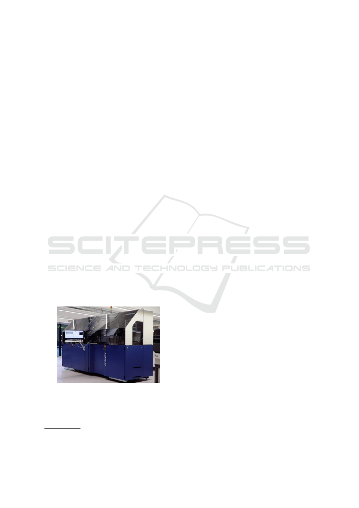
Figure 2 illustrates the overall die bonder process.

On its journey, a die gets transported to different pro-

cessing stations. At the ﬁrst processing station, the

die is picked up. At the second station, it gets in-

https://www.itecequipment.com/products

spected for quality; these quality inspections may in-

volve visual inspections for damage or testing of the

die. There are optional processing stations, at which a

die gets ﬂipped and subsequently inspected again. At

the last processing station, the die gets attached to a

lead frame. Between the operations on the die, there

are index steps which transport the die to the next pro-

cessing station.

To obtain the desired high productivity, the oper-

ations at the ADAT3-XF’s processing stations run in

parallel. Figure 2 shows that ﬁve dies are processed

in parallel at the ﬁve stations (Pick-up, Inspect 1, Flip,

Inspect 2, Attach). To allow this kind of pipelined

parallelism, die operations and die transfers need to

be synchronized. Similarly, the indexing steps of the

wafer table between die pick-ups and those of the

product holder between die attachments need to be

synchronized with the die transfer and die operations.

Our goal is to quickly and accurately predict the

productivity of the different variants of the ADAT3-

XF die bonder family. This is challenging because

of the system variability. The variability in the die

bonder product family can be described in terms of

Product, Process and Resource (Meixner et al., 2019).

Product. A source of product variability is the char-

acteristics of the dies being processed, e.g. their di-

mensions. Another source of product variability is

the lead frame to which the dies are attached; this

includes the lead frame’s substrates (i.e. reel, strip,

panel, web).

Process. The lead frame deﬁnes the correspond-

ing bonding technique (glue, eutect), and the places

where to attach dies. Both inﬂuence the process re-

alized by a die bonder, i.e. the steps needed to attach

the dies to the lead frame. Another source of pro-

cess variability is the pipeline (see Figure 2), e.g. the

number and type of quality inspections performed and

whether dies need to be ﬂipped.

Resource. The lead frame also inﬂuences resource

variability, because each substrate has its own product

holder. Besides the product holder, resource variabil-

ity includes components with different timing charac-

teristics, e.g. components running at different speeds:

the ADAT3-XF family includes variants implement-

ing the same process, but at different speeds.

4 SINGLE SYSTEM MODELING

As a stepping stone for introducing productivity mod-

eling for the family of die bonders, we modeled one

variant. A die bonder is a mechatronic systems with

a repetitive steady-state behavior. To predict the vari-

ant’s productivity, we created a productivity model of

MODELSWARD 2023 - 11th International Conference on Model-Based Software and Systems Engineering

228

Figure 2: ADAT3-XF die bonder process pipeline.

its steady-state behavior. We distinguish the creation

of the model (see Section 4.1) and the validation of

the model’s correctness (see Section 4.2). As creating

an accurate model is not a ﬁrst-time-right process, we

needed to perform both steps several times.

4.1 Model Creation

LSAT

is a tool to specify and analyze the logistics

of cyber-physical production systems (van der Sanden

et al., 2021). LSAT is especially meant for modeling

the deterministic logistics of production systems like

ITEC’s die bonders. Using LSAT, one speciﬁes a sys-

tem in terms of a platform and an application (see Fig-

ure 3). The platform describes the system’s resources

and the functionality they provide; the application de-

scribes the system’s behavior by combining resource

functionality.

Figure 3: LSAT model structure (adapted from (van der

Sanden et al., 2021)).

Platform: To model the platform, we need to spec-

ify a machine model and a settings model. LSAT’s

machine models specify the resources with their pe-

ripherals, and the actions and movements that these

peripherals can perform. The resources mainly in-

volve the components needed to realize steps of a de-

sired process, but they also include synchronization

resources. Synchronization resources are used e.g. to

avoid collisions between components that move in the

same space. Figure 4 shows the resources and the pe-

ripherals of the model of a simpliﬁed ADAT3-XF sys-

tem. The main resources are the wafer table, the push-

up unit, the die transfer, two Z-motors, and the prod-

uct holder. In addition, there are two synchronization

resources to model dependencies between the opera-

tions performed during the journey of a die. Also part

of the machine model, but not shown in Figure 4, are

https://www.eclipse.org/lsat/

the actions and movements that the resources’ periph-

erals can perform.

Figure 4: ADAT3-XF machine model.

LSAT’s settings models capture the physical char-

acteristics of the machine, including the physical co-

ordinates and motion proﬁles describing motor move-

ments. Settings model specify the characteristics of

the machine model’s peripherals; Figure 5 shows part

of the simpliﬁed ADAT3-XF system’s settings model.

It contains durations for peripheral actions as well as

motion parameters and physical locations for motor

movements.

Figure 5: ADAT3-XF settings model.

Application. On its journey, a die gets picked up from

a diced wafer on the wafer table, it visits several pro-

cessing stations for (quality inspection) process steps,

and it gets attached to a lead frame on the product

holder. The transfer of the dies between process lo-

cations is called indexing. Between two consecutive

pick-up steps, the wafer table also makes an indexing

step to allow the next die to be picked up. Similarly,

the product holder makes indexing steps between at-

tach operations. To describe a system’s application,

these operations and the transportation in between are

Experiences and Lessons from Introducing Model-Based Analysis in Brown-Field Product Family Development

229

described as activities in LSAT’s activity models. Ac-

tivities are directed acyclic graphs consisting of pe-

ripheral actions as deﬁned in the machine model.

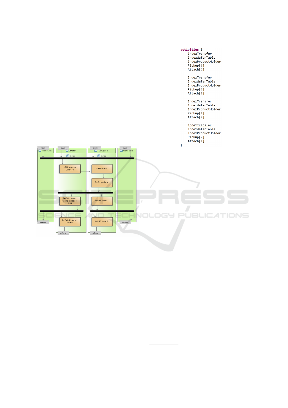
LSAT’s activities describe the operations per-

formed. An example is the pick-up activity shown in

Figure 6. This activity involves two active resources,

i.e. ZMotor and PushupUnit, and two resources that

are used for synchronization, i.e. PickupLock and

WaferTable. The activity diagram shows that the Z-

motor is extended, after which the needle extends and

pushes a die on the Z-motor’s collet. After this die

transfer, the Z-motor and the needle retract simulta-

neously. The synchronization resources get released

during the retraction of the Z-motor and the needle.

At this point in the retraction, the die transfer and the

wafer table can safely start their index step. This par-

allelism increases the system’s productivity.

Figure 6: ADAT3-XF pick-up activity.

LSAT’s logistics models combine activities into a

desired overall system process. The dispatching se-

quence shown in Figure 7 describes a four cycles of

the simpliﬁed ADAT3-XF conﬁguration. Each cycle

involves indexing of the die transfer, the wafer table

and the product holder, followed by pick-up and at-

tach activities. Note the the pick-up and attach ac-

tivities are parameterized; their parameters indicate

which Z-motor is used.

The activities in a dispatching sequence interact

via the resources that they share (van der Sanden

et al., 2021): if an activity shares a resource with a

preceding activity, the activity’s actions involving this

shared resource can only start after the preceding ac-

tivity has released the resource. If activities do not

share any resources, they can run in parallel.

Figure 8 shows the result of running LSAT’s tim-

ing analysis, i.e. a Gantt chart of the four machine

Figure 7: ADAT3-XF logistics model.

cycles in Figure 7. The Gantt chart shows the actions

performed by the system’s peripherals over time. In

this Gantt chart, the low blocks represent resources

being claimed by activities and the high blocks the

actions and movements executed by the peripher-

als; arrows represent the sequence dependencies be-

tween the peripheral actions, the peripheral move-

ments, the resource claims and the resource releases.

The blocks’ colors correspond to the involved activi-

ties. As the indexing activities (red) of the wafer ta-

ble, transfer, product holder do not share resources,

they run in parallel. The same holds for the pick-up

(blue) and attach (green) activities. This corresponds

to the pipeline behavior shown in Figure 2.

4.2 Model Validation

We based the modeling described in Section 4.1 on

available documentation and knowledge of ITEC’s

domain experts. As it is difﬁcult to obtain a com-

plete system speciﬁcation from these ambiguous and

incomplete sources of information, it is essential to

validate the model before using the model to predict

the system’s productivity. We validated the LSAT

model by comparing the model’s execution traces to

the system’s. We did this using TRACE4CPS

(Hen-

driks et al., 2017). This is a tool, which is used in-

side LSAT to visualize model execution traces, but

which also allows analysis and comparison of execu-

tion traces as well as run-time veriﬁcation.

Figure 9 shows a small part of the system’s exe-

cution trace, after translating it to the TRACE4CPS

https://www.eclipse.org/trace4cps/

MODELSWARD 2023 - 11th International Conference on Model-Based Software and Systems Engineering

230

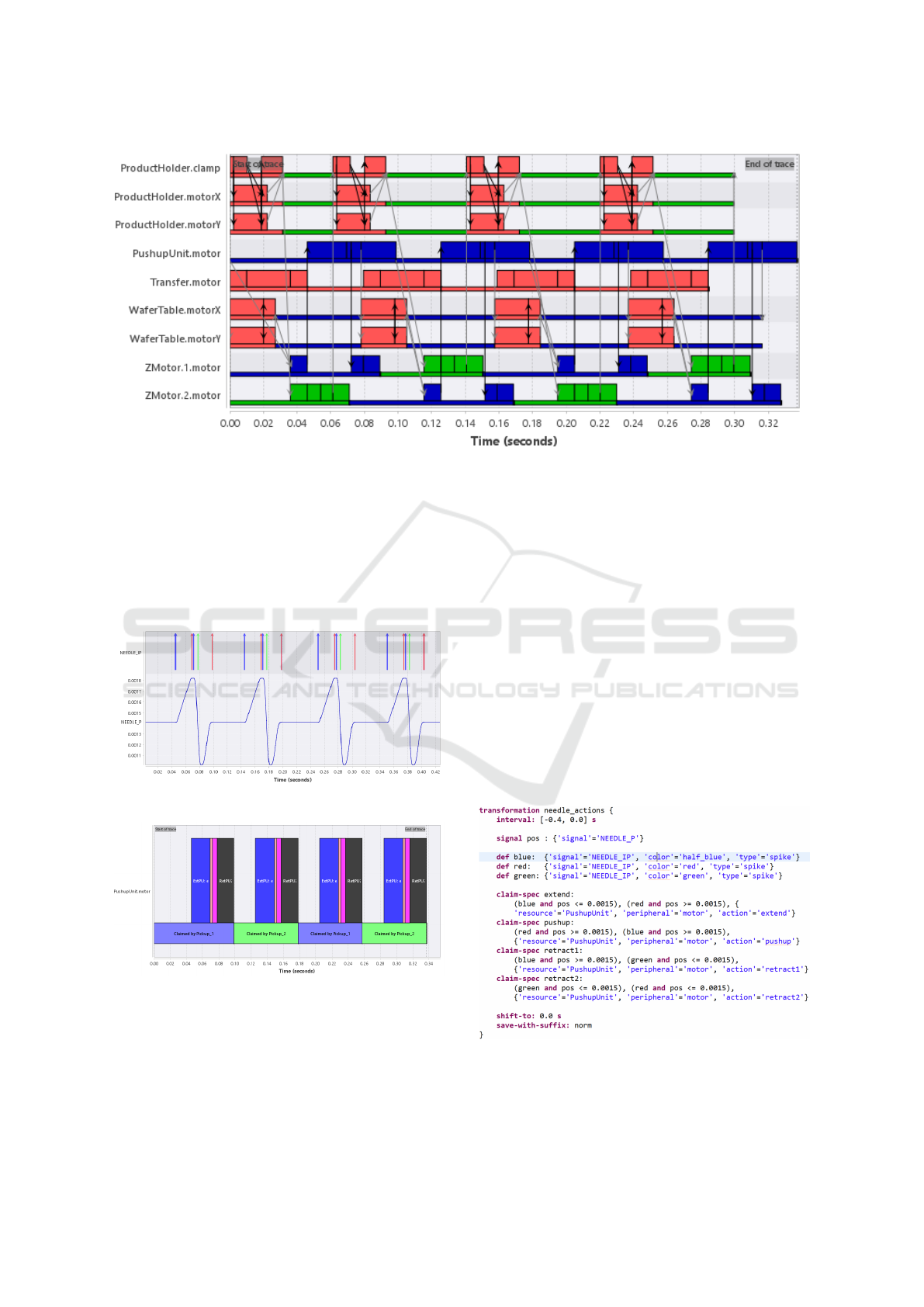
Figure 8: Gantt chart of four ADAT3-XF machine cycles.

format using an ITEC-proprietary tool. A swim lane

shows either a continuous signal representing a motor

position or discrete events. Figure 10 shows the cor-

responding part of the model’s execution trace: multi-

ple executions of the actions of the push-up unit when

picking up a die (the blocks in the PushupUnit.motor

swim lane in Figure 8).

Figure 9: System execution trace (in TRACE4CPS).

Figure 10: Model execution trace.

Clearly, one cannot directly compare the execu-

tion traces in Figures 9 and 10; the information in the

system’s execution trace is more detailed than that in

the model’s. To unify the abstraction level of the ex-

ecution traces, we have created and applied a trans-

formation language based on TRACE4CPS’ run-time

veriﬁcation functionality. We use the system execu-

tion trace in Figure 9 as an example. This ﬁgure

shows the events and signals corresponding to a nee-

dle pushing a die from the wafer onto a Z-motor’s col-

let. The top swim lane shows the needle motor events,

the bottom swim lane the position of the needle. Red

and blue events correspond to starting and stopping

the motor; green events are sent when a certain posi-

tion is reached. The needle performs a sequence of

four actions: (1) extension, (2) push up, (3) partial

retraction, and (4) full retraction. Using the rules in

Figure 11, we derive the start and end of these ac-

tions from the execution trace in Figure 9. The rules

combine an event color and a needle position to deter-

mine the start and end of the model’s needle actions.

Figure 12 shows the resulting execution trace after ap-

plying the rules in Figure 11.

Figure 11: Transformation speciﬁcation.

The Gantt chart in Figure 12 strongly resembles

the needle actions shown in Figure 10. When apply-

Experiences and Lessons from Introducing Model-Based Analysis in Brown-Field Product Family Development

231

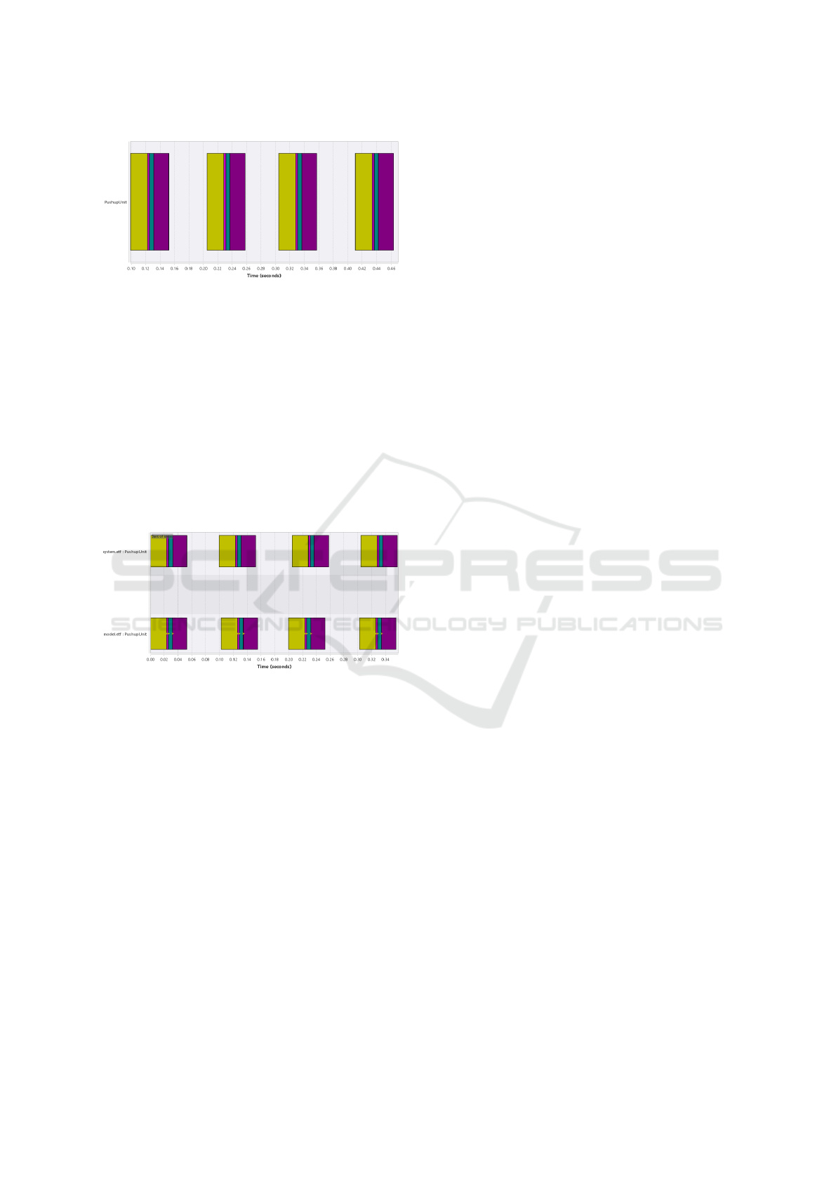
Figure 12: Transformation output.

ing another transformation on the Gantt chart in Fig-

ure 10, we obtain a Gantt chart with only the model’s

needle actions (the high blocks in Figure 10), leaving

out the resource claims (the low blocks in Figure 10).

Both transformed Gantt charts can be compared in

TRACE4CPS by opening them simultaneously. This

is shown in Figure 13. One can easily see that the or-

der of the needle actions are identical in both Gantt

charts. For more complex Gantt charts, this may

be less obvious. Then, one can TRACE4CPS’ trace

comparison for this sequence check. In addition,

TRACE4CPS’ timing analysis was used to show that

the durations of the actions was identical.

Figure 13: Gantt chart comparison.

Despite the matching action sequence and match-

ing action durations, the total duration of the sys-

tem’s execution trace (top) is slightly longer than the

model’s (bottom). In other words, the model was

valid on an individual action level, but not on an over-

all level. The difference of the total duration was

caused by a delay in the system: the system’s motion

controller introduces a small delay between issuing a

start signal and the actual start of the motor. Because

we did not include this delay in the model, this caused

a delay which slowly builds up over time, as one can

see in Figure 13.

In subsequent models, we captured the delay be-

tween the start signal and the motor start in two man-

ners: (1) for actions speciﬁed using motion proﬁles, a

motion proﬁle was introduced including a short start

delay and (2) for actions without motion proﬁles, a

motion controller delay action was introduced. With

these changes, the system and model had both the

same dependencies and the same durations. In other

words, we obtained a valid model, i.e. a model whose

behavior accurately matches the system’s behavior.

Such a model can be used as a starting point for ex-

ploring yet-to-be-developed variants.

5 PRODUCT FAMILY MODELING

There are many variants of ADAT3-XF die bonders.

The systems in this family share resources; e.g. the

die transfer, the Z-motors and the wafer table are used

in most system variants. Similarly, activities may be

shared by multiple variants; if two variants share the

wafer table, they may also share the pick-up activities

and if they share the same product holder, they may

also share the attach activities. On the other hand,

there are differences with respect to the number of

dies in the system’s pipeline, the quality inspections

being performed, the dimensions of system compo-

nents, and the speeds of the peripherals.

To facilitate the reuse and variability of the

ADAT3-XF system family, we created a master model

in LSAT and a corresponding master transformation

in TRACE4CPS. The master model is a collection of

LSAT models providing a library of LSAT model ele-

ments; the master transformation is a library of trans-

formation rules that can be used to translate model

and variant execution traces to a uniﬁed form.

The master model describes the resources and pe-

ripherals of all ADAT3-XF system conﬁgurations in-

cluding the peripheral actions and these actions’ set-

tings. The master model also speciﬁes all conﬁgu-

rations’ activities. Because of the desired reuse, the

master model’s activities became more ﬁne-grained

than those of the individual variants. For instance, the

(simpliﬁed) variant’s pick-up activity shown in Fig-

ure 6 was decomposed into separate activities of the

Z-motors and the push-up unit with synchronization

resources to keep the desired logistic process. One

of these activities is shown in Figure 14. It describes

how the extension of a Z-motor to the wafer table.

Beside the Z-motor resource, it involves two synchro-

nization resources to avoid other activities from start-

ing too early.

To facilitate reuse of model elements, the master

model was made in a modular fashion following the

component structure of the system variants. Figure 15

visualizes the master model structure in relation to

the product family structure. Each system variant has

a dedicated logistics model with the appropriate ac-

tivity dispatching sequence. A logistics model of an

ADAT3-XF system variant uses activities from the ac-

tivity models describing the activities of the variant’s

MODELSWARD 2023 - 11th International Conference on Model-Based Software and Systems Engineering

232

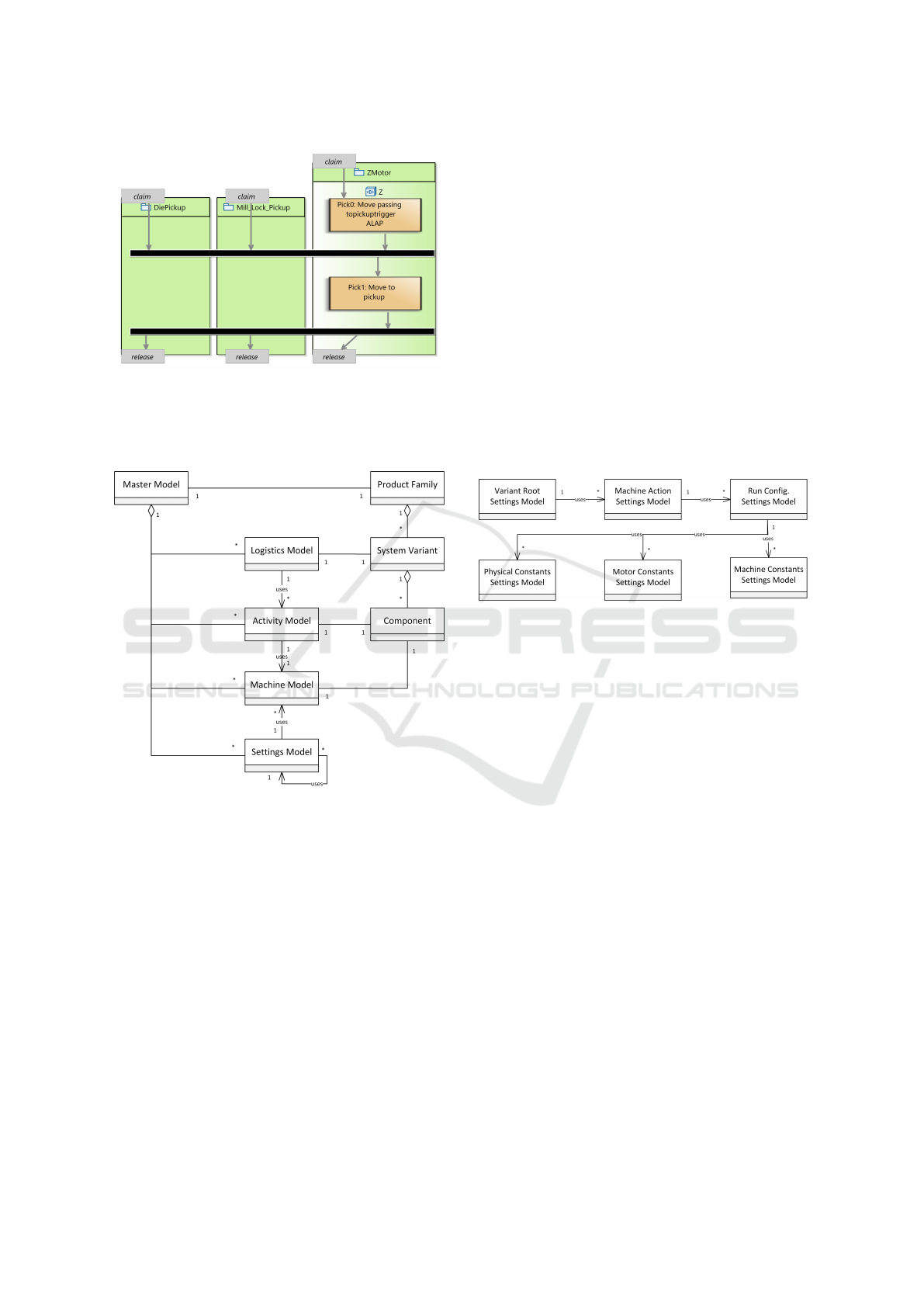
Figure 14: Reusable activity element.

components. These activity model uses the machine

models of the resources used in their activities. Ma-

chine models do not use other types of models.

Figure 15: Master model structure.

Per system component, the master model contains

a single machine model and a single activity model.

The former describes the component in terms of re-

sources and peripherals; the latter describes the activ-

ities with this component as the main resource. For

instance, the machine model of the push-up unit de-

scribes the motors of the push-up unit and the cor-

responding activity ﬁle describes the needle’s exten-

sion, push-up and retraction activities.

Because of the diversity of settings, modularity

and reuse of settings models proved more complex

than for machine and activity models. Settings mod-

els are used to determine the duration of peripheral

actions. Durations are either speciﬁed as ﬁxed values

or they are derived from a description of a movement.

For movements, settings models contain information

about distance, velocity, acceleration, and jerk. Both

types of settings can be speciﬁed as (closed) expres-

sions containing settings in other settings models.

The usage relation of the master model’s settings

models is shown in Figure 16. This is a layered struc-

ture with settings models for machine, motor, and

physical constants forming the lowest layer. Machine

constants settings models describe the physical char-

acteristics of available resources, motor constants set-

tings models include the parameters of the peripher-

als’ motion proﬁles, and physical constants settings

models include the variables that are not coupled to a

resource or peripheral. The second layer contains the

run conﬁguration settings models that are speciﬁed in

terms of the lowest layer’s constants. The run con-

ﬁguration settings are used in the settings models of

the peripheral actions, which are combined in a single

root settings model of a system variant.

Figure 16: Settings models structure.

6 LESSONS LEARNED

In Sections 4 and 5, we have outlined our work of in-

troducing productivity modeling in brown-ﬁeld prod-

uct family development. This section describes the

lessons that we have learned while developing pro-

ductivity models of a family of die bonder systems.

We distinguish modeling lessons (see Section 6.1) and

organizational lessons (see Section 6.2).

6.1 Modeling Lessons

Parameterization. The ADAT3-XF systems are high-

productivity machines that handle tens of thousands

of products per hour. To obtain such high produc-

tivity, the systems support a pipelined execution (see

Figure 2). To allow parallel handling of the products

in the pipeline, the system contains multiple resources

of the same type. For instance, multiple Z-motors are

used to pick up one die and, in parallel, attach an-

other. To keep the model of a system variant concise,

we learned that parameterization of resources and ac-

tivities is essential. Parameterized activities use pa-

rameterized resources and are used multiple times in a

dispatching sequence (see Figure 7). Without param-

Experiences and Lessons from Introducing Model-Based Analysis in Brown-Field Product Family Development

233

eterization, a system variant model would be much

longer and its maintenance would involve a large ef-

fort as one needs to keep all instances consistent. In

the context of a family of system variants, parameter-

ization becomes even more important as it involves

even more reuse.

Modularity vs. Understandability. To maximize reuse

in product family modeling (see Section 5), we noted

that the model elements became smaller. This espe-

cially holds for the activities describing the system be-

havior. By dividing one activity into multiple smaller

activities, one has to take care of the dependencies

that were captured by the original activity. In our use

case, this meant the introduction of additional syn-

chronization resources in the decomposed activities

that replace the cut precedence constraints in the orig-

inal activity. The smaller activities increase model el-

ement reusability, but we observed that the introduced

synchronization resources reduce model understand-

ability and maintainability. To improve the situation,

we advice to use another synchronization concept of

LSAT: activities can synchronize either via shared re-

sources or via events. The latter can be used to sig-

nal that e.g. actions have completed. These events are

more natural to system developers than the synchro-

nization resources.

Variation Modeling. By making the step from indi-

vidual systems to a family of systems, we learned that

tools intended for individual systems cannot just be

used for families of systems.

In our use case, we used LSAT to create a master

model consisting of reusable model elements. LSAT’s

support for modularity proved adequate for its ma-

chine and activity models. However, we experienced

that this is not true for its settings models. To allow

reuse of LSAT’s settings models, we needed a com-

plex hierarchy of settings models (see Figure 16). In

this hierarchy, elements inﬂuencing the whole system

are on the lowest level. In order words, the hierarchy

of settings models does not follow a normal hierarchy

pattern, in which the lowest levels have the smallest

inﬂuence.

Our use case showed the difﬁculties that one faces

when introducing a model-based way of working in

a brown-ﬁeld development situation. We learned that

we needed to address many challenges to come to a

working solution. We could have overcome some of

the challenges by handling system variability differ-

ently: e.g. we could use variability modeling tools

like pure::variants

or FeatureIDE

to describe all

possible variability and to generate variant productiv-

ity models from.

https://www.pure-systems.com/

https://www.featureide.de/

Model Validation by Abstraction. During model val-

idation, we faced the challenge that the systems’ ex-

ecution logs are more detailed than the models’. The

systems’ execution logs contain all motor start and

end signals, but they do not show which action starts

or ends. To overcome this difference, we raised the

abstraction level of the systems’ execution log using

a set of transformation rules similar to those in Fig-

ure 11. After applying these rules to a variant’s ex-

ecution trace and the corresponding model execution

trace, we could use TRACE4CPS’ comparison func-

tionality to validate model correctness.

Reuse of Validation Rules. We learned that reuse of

these transformation rules is not straightforward for

different instances of the same system. The distances

traveled by the motors of a system differ per system,

even if they have the same conﬁguration. As the mo-

tor positions are used to do model validation, we ob-

served that one needs to carefully consider the magic

numbers in the transformation rules. These should

match the characteristics of the system used for model

validation. This is even more challenging for a family

of system variants, as their magic numbers may also

vary across different variants.

Incremental Model Validation. Before we could use

the models to predict the productivity of system vari-

ants, they needed to be validated. We learned that

an incremental model validation approach was very

effective. The transformation rules used in the mas-

ter transformation guaranteed the correctness of (the

timing of) the model elements. Having the model ele-

ments validated allowed us to focus on the validation

combinations of model elements. As the second step,

we validated the timing and order of the actions of

each peripheral using TRACE4CPS’ trace compari-

son functionality. Finally, we used the same function-

ality to validate the timing and order of the actions of

the entire model.

We noted that over time the differences between

the system and the model became more and more sub-

tle, requiring more and more domain knowledge. A

clear example is the delay between start signal and

motor start discussed in Section 4.2. Although this is

visible for individual peripherals (see Figure 13, we

only identiﬁed the cause after observing the timing

difference throughout the entire execution trace.

6.2 Organizational Lessons

System and Model Co-Evolution. In this paper, we

described how we introduced a master model and a

corresponding master transformation for the family

of ITEC’s ADAT3-XF die bonders. This required a

signiﬁcant effort, but we also realized that this effort

MODELSWARD 2023 - 11th International Conference on Model-Based Software and Systems Engineering

234

does not stop here. The family of die bonders will

change over time: faster variants of existing conﬁgu-

rations will be introduced as well as variants applying

new technology. To avoid that the efforts made to cre-

ate the master model and model transformation are

wasted, the master model and model transformation

should co-evolve with the product family. This re-

quires embedding the master model and model trans-

formation in the way of working of the organization.

Ideas to achieve this include (1) putting the master

model and master transformation under version con-

trol just like the source code, (2) making the model

and transformation part of the system documenta-

tion, and (3) annotating the system’s source code with

knowledge about the master model and master trans-

formation. The latter would also greatly simplify the

speciﬁcation of transformation rules.

System Changes for Modeling. When specifying the

rules to validate our models, we observed that some

rules were quite complex and hence hard to reuse. In-

stead of specifying complex model validation rules,

we think it is more convenient to adapt the system for

the purpose of predictive modeling. E.g. the events in

a system execution log could be extended with infor-

mation about the corresponding model action. By ex-

tending the system’s execution logs with knowledge

of the corresponding model, (1) there is an explicit

mapping between the system and the correspond-

ing variant model, (2) transformation rules become

simpler and the master transformation more main-

tainable, and (3) model validation becomes (more)

straightforward.

Democratization of Knowledge. In Section 4, we ex-

plained how we modeled individual system variants.

To create valid LSAT models for ADAT3-XF sys-

tems, we started modeling an existing system vari-

ant. We created the variant model by capturing ex-

pert knowledge and comparing model and system ex-

ecution traces. The model creation and validation ex-

plained in Section 4 showed that our approach was

an iterative one: the differences identiﬁed by com-

paring Gantt charts revealed information that was not

yet captured by the model. It was challenging to cap-

ture all dependencies, especially those between ac-

tions of peripherals of different resources. By even-

tually obtaining a validated model, the model and

the corresponding transformation rules became a non-

ambiguous source of domain knowledge. ITEC engi-

neers saw this as a valuable asset to transfer (implicit)

domain knowledge in experts’ heads to new employ-

ees.

Tool Usability. In our use case, we have used LSAT

and TRACE4CPS to introduce productivity model-

ing for a family of die bonder systems. Both LSAT

and TRACE4CPS use textual domain-speciﬁc lan-

guages (DSLs) to specify model elements. The in-

tended users of of LSAT and TRACE4CPS within

ITEC have a background in mechanical engineering.

We found out that they are not familiar with tex-

tual interfaces. Creating instances of textual DSLs

was said to feel like software development. A way

to overcome this usability issue is to develop (possi-

bly graphical) company-speciﬁc tooling that hides the

perceived complexity of the existing languages.

Model-Based System Validation. In this paper, we

have used transformation and comparison of execu-

tion traces to validate our productivity models. A

validated model can be used to explore the behav-

ior of yet-to-be-developed system variants (Parappu-

rath et al., 2013). At the end of this exploration, the

model provides a (partial) speciﬁcation for the sys-

tem. In other words, the role of model changes from

descriptive to prescriptive. We realized that the exe-

cution trace comparison techniques can also be used

to validate system behavior: by comparing uniﬁed

system and model execution traces, one can validate

whether the system’s behavior is as the model pre-

dicts/prescribes.

7 CONCLUSION

In this paper, we have introduced a model-based way

of working in brown-ﬁeld product family develop-

ment. The paper presents two results: (1) we devel-

oped (a) a master model, i.e. a library of model el-

ements matching the elements of the product family

and (b) a master transformation, i.e. a library of trans-

formation rules to transform system and model execu-

tion traces to a uniﬁed form, and (2) we reﬂect on the

process of introducing a model-based way of working

by presenting experiences and lessons learned.

The use case shows that it is feasible to introduce

a model-based way of working in brown-ﬁeld product

family development. It also shows that model-based

development of a product family is signiﬁcantly more

complex than for an individual system. Many chal-

lenges need to be addressed: for a successful intro-

duction of a model-based way of working, changes

are required both on the system development side and

on the modeling side. Some of these challenges are

purely technical, but most (also) have a signiﬁcant or-

ganizational aspect: to maintain a model-based way

of working on the long run, changes are required in

the system and in the organization.

Experiences and Lessons from Introducing Model-Based Analysis in Brown-Field Product Family Development

235

The use case’s master model and master trans-

formation introduce the beneﬁt of being able to pre-

dict the productivity of yet-to-be-development sys-

tem variants. The use case shows that the beneﬁts

of model-based way of working are not limited to

this. Beside the prediction beneﬁt, our use case re-

veals two additional beneﬁts of the master model and

master transformation: (1) they capture knowledge

in experts’ heads and (2) they provide an additional

means to validate systems.

ACKNOWLEDGEMENTS

The research is carried out as part of the Bright pro-

gram under the responsibility of TNO-ESI with ITEC

as the carrying industrial partner. The Bright research

is supported by the Netherlands Organisation for Ap-

plied Scientiﬁc Research TNO.

REFERENCES

Czarnecki, K. and Eisenecker, U. W. (2000). Genera-

tive Programming: Methods, Tools, and Applications.

Addison-Wesley, Reading, MA, USA.

Feng, Y., Dreef, K., Jones, J. A., and van Deursen, A.

(2018). Hierarchical abstraction of execution traces

for program comprehension. In 26th Conference on

Program Comprehension (ICPC ’18), pages 86–96,

Gothenburg, Sweden.

Gad, R. (2017). Improving packet capture trace import in

Trace Compass with a data transformation DSL. In

2017 IEEE 41st Annual Computer Software and Ap-

plications Conference (COMPSAC 2017), volume 2,

pages 7–12, Turin, Italy.

onniger, H., Krahn, H., Pinkernell, C., and Rumpe, B.

(2008). Modeling variants of automotive systems us-

ing views. In Klein, T. and Rumpe, B., editors, Mod-

ellbasierte Entwicklung von eingebetteten Fahrzeug-

funktionen, number 2008-01 in Informatik-Berichte,

pages 76–89. Technische Universit

at Braunschweig,

Braunschweig, Germany.

Hendriks, M., Verriet, J., Basten, T., Theelen, B., Brass

M., and Somers, L. (2017). Analyzing execution

traces: Critical-path analysis and distance analysis.

International Journal on Software Tools for Technol-

ogy Transfer, 19(4):487–510.

Hoffman, C. M. and Joan-Arinyo, R. (1998). CAD and

the product master model. Computer-Aided Design,

30(11):905–918.

Kang, K. C., Cohen, S. G., Hess, J. A., Novak, W. E., and

Peterson, A. S. (1990). Feature-oriented domain anal-

ysis (FODA) feasibility study. Technical report, Soft-

ware Engineering Institute, Carnegie-Mellon Univer-

sity, Pittsburgh, PA, USA.

Meixner, K., Rabiser, R., and Bifﬂ, S. (2019). Towards

modeling variability of products, processes and re-

sources in cyber-physical production systems engi-

neering. In 23rd International Systems and Soft-

ware Product Line Conference (SPLC ’19), volume B,

pages 49–56, Paris, France.

Parappurath, V. V., Voeten, J. P. M., and Kotterink, K. C.

(2013). Calibration error bound estimation in perfor-

mance modeling. In 2013 Euromicro Conference on

Digital System Design, pages 97–102, Los Alamitos,

CA, USA.

Reiss, S. P. (2005). Dynamic detection and visualization of

software phases. In Third International Workshop on

Dynamic Analysis (WODA ’05), pages 1–6, St. Louis,

MI, USA.

Sandberg, M., Tyapin, I., Kokkolaras, M., Isakasson,

O., Aidanp

a, J.-O., and Larsson, T. (2011). A

knowledge-based master-model approach with appli-

cation to rotating machinery design. Concurrent En-

gineering, 19(4):295–305.

Tawhid, R. and Petriu, D. (2008). Integrating performance

analysis in the model driven development of software

product lines. In Czarnecki, K., Ober, I., Bruel, J.-

M., Uhl, A., and V

olter, M., editors, MODELS 2008:

Model Driven Engineering Languages and Systems,

pages 490–504. Springer, Berlin, Heidelberg.

van der Linden, F. J., Schmid, K., and Rommes, E. (2007).

Software Product Lines in Action: The Best Indus-

trial Practice in Product Line Engineering. Springer-

Verlag, Berlin, Heidelberg.

van der Sanden, B., Blankenstein, Y., Schiffelers, R., and

Voeten, J. (2021). LSAT: Speciﬁcation and analysis

of product logistics in ﬂexible manufacturing systems.

In 2021 IEEE 17th International Conference on Au-

tomation Science and Engineering (CASE), pages 1–

8, Lyon, France.

Verriet, J., Dankers, R., and Somers, L. (2018). Per-

formance prediction for families of data-intensive

software applications. In Companion of the 2018

ACM/SPEC International Conference on Perfor-

mance Engineering (ICPE ’18), pages 189–194,

Berlin, Germany.

MODELSWARD 2023 - 11th International Conference on Model-Based Software and Systems Engineering

236