Ongoing Work to Study the Underlying Statistical Patterns of

Oesophageal Chromothripsis

Jack Fraser-Govil and Zemin Ning

The Wellcome Sanger Institute, Wellcome Genome Campus, Hinxton, Cambridge CB10 1SA, U.K.

Keywords:

Chromothripsis, Bayesian Statistics, Chromosome Rearrangement.

Abstract:

In this position paper we demonstrate our ongoing efforts to develop and test a number of statistical tools

and methedologies which allow us to study the underlying statistical properties of a genetic sequence which

has undergone chromothripsis, and hence provide some novel probes into the mechanisms which cause such

catastrophic genomic rearrangement. Using these tools, we study an oesophogeal cancer sample showing more

than 1000 rearrangements, with 800 of these on chromosome 6. By studying this chromosome, we challenge

a prevalent idea within the literature: that chromothripsis breakpoints are non-random, ﬁnding instead that

despite a high degree of clustering, the clusters themselves are uniformly distributed across the chromosome.

We also show that although 3-dimensional proximity is a tempting explanation for the rearrangement pattern,

the statistical evidence does not favour it at the current time. In addition, we attempt to disambiguate some of

the terminology surrounding chromothripsis.

1 INTRODUCTION

The conventional model of cancer development posits

that the inciting genetic defects are the result a grad-

ual accumulation of point mutations and rearrange-

ments, eventually resulting in the activation of onco-

genes. The discovery of chromothripsis (Stephens

et al., 2011), however, presented a potential alterna-

tive pathway: that of a genetic crisis resulting in a

massive genomic rearrangement in a single event.

The chromothripsis phenomomenon was charac-

terised by a number of ‘breakpoints’ which showed

an unusual level of clustering, and an oscillation in the

copy number variation which seemed to indicate that

the genome had been ‘shattered’ into multiple distinct

fragments, before a DNA repair mechanism had erro-

neously repaired these broken links into a contiguous

but now cancer-causing sequence.

The view that chromothripsis is the result of a sin-

gle catastrophic event has, however, been challenged

(Solorzano et al., 2013). This is complicated further

by that fact that some (i.e. (Korbel and Campbell,

2013)) use simultaneity as an axiomatic part of their

deﬁnition of chromothripsis - which in turn precludes

the study of any evidence of chromothripsis as an ex-

tended process. We therefore emphasise throughout

this work the importance of using a constent termi-

nology, which we robustly deﬁne in section 1.1.

The actual underlying mechanics of chromothrip-

sis, whether they be instantaneous or sequential, or

even if multiple such pathways exist, remain an open

question. The aim of our ongoing work is to use sta-

tistical tools to attempt to gain insight into the ways

in which the breakage and repair processes imprint

themselves onto the resulting cancer genome, using

a particularly prominent oesophogeal cancer as our

testbed for these tools.

In doing so, we introduce a Bayesian inference

engine (which will be published as its own separate

work, (Fraser-Govil, 2023)), and discuss our ongoing

work to use this tool to study the break process using

the CHROMOSPA tool, and then ﬁnally leveraging the

statistical engine to identify if the repair process can

be associated to spatial proximity within the nucleus,

using HiC data.

This is ongoing work, so our conclusions and data

are provisional for the moment, but we hope that this

elucidates the direction and motivations of our re-

search.

1.1 Terminology

As noted, the terminology surrounding chromothrip-

sis has developed and shifted since its discovery, with

some explanatory features present in the original stud-

ies since being used as deﬁnitional elements. It is

therefore vital when discussing chromothripsis that

one is careful to deﬁne exactly what one means by

that term.

In our work, we emphasise that chromothripsis

276

Fraser-Govil, J. and Ning, Z.

Ongoing Work to Study the Underlying Statistical Patterns of Oesophageal Chromothripsis.

DOI: 10.5220/0011785600003414

In Proceedings of the 16th International Joint Conference on Biomedical Engineering Systems and Technologies (BIOSTEC 2023) - Volume 3: BIOINFORMATICS, pages 276-283

ISBN: 978-989-758-631-6; ISSN: 2184-4305

 2023 by SCITEPRESS – Science and Technology Publications, Lda. Under CC license (CC BY-NC-ND 4.0)

Ostracon

Chromothripsis

Hologenome

Mignogenome

Figure 1: A Diagram indicating our chosen terminology for

chromothripsis.

is a phenomenological term, describing an observed

pattern in the data. Formally speaking, we deﬁne

chromothripsis as a process which generates a large-

scale genomic rearrangement which possesses statis-

tical indiators (i.e. copy number oscillations, cluster-

ing) which lie in tension with the standard, sequential

mechanism of cancer evolution.

This deﬁnition is intentionally ambivalent to the

precise mechanism by which chromothripsis oper-

ates - either by the original ‘shattering’ model, or

by some extended process which nevertheless oper-

ates distinctly from the previously understood mech-

anisms of cancer formation.

In keeping with our efforts to use clear terminol-

ogy, we also provide the following deﬁnitions to al-

low us to unambiguously distinguish between the key

components of chromothripsis:

• Hologenome (also Holosequence etc.): The origi-

nal, unbroken genetic sequence

• Mignogenome (also Mignosequence etc.), the se-

quence which has been drastically rearranged by

the process of chromothripsis.

• Ostracon, an individual unbroken, contiguous,

segment of the hologenome present within the

mignogenome (from ὄστρακον, broken fragment

of pottery with letters inscribed)

• Breaks (also breakpoints), the points on the

Hologenome which form the original edges of

the ostracons, speciﬁed through a single coordi-

nate: that of the chromosomal coordinate in the

hologenome.

• Joins (also joinpoints), the points on the

Mignogenome which form the edges of adjoining

ostracons in the mignogenome

Under this terminology, therefore, chromothripsis

is the generic name given to any process which gener-

ates a mignogenome, either by shattering the genome

into ’ostracons’ which are then reassembled, or by a

more extended process which simply mimics this be-

haviour.

We emphasise that there is a distinct and important

difference between the locations of ostracons within

the hologenome and their location in mignogenome,

and that there are potentially two different driving

forces behind them.

The location of ostracons (or, more precisely,

the edges of the ostracons - the breaks) within the

hologenome are a result of the destructive process:

the process broke the hologenome at several loca-

tions, and patterns in the individual positions of the

breakpoints are characteristic of this process.

The location of ostracon pairs within the

mignogenome, however, is indicative of the repair

process - the process which repaired the genome after

the shattering event. Patterns in which pairs of ostra-

cons are adjacent are indicative of how this process

occured.

We have no particular a priori reason to assert that

these processes are related, and thus we should study

them as distinct - though sequential - processes.

2 DATA

2.1 Identiﬁcation of Breakpoints

We used STEPPINGSTONE

to parse the reads of

the oesophogeal cancer samples, and extract a list

of identiﬁed breakpoints. STEPPINGSTONE func-

tions by noting that when reads originating from a

mignogenome are aligned to a reference, the edges of

the ostacons will appear as chimeric reads – with the

sequences on either side of the joinpoint aligning to

different parts of the genome – even though they are

genuinely contiguous sequences in the mignogenome.

STEPPINGSTONE reports these chimeric points

via the two chromosomal coordinates within the

hologenome that the chimeric reads correspond to.

Work is ongoing to fully assemble this information

to generate the full mignogenome sequence.

2.2 Test Sample

For the current work-in-progress demosntrated in this

work, we use the sequencing data of an oesophogeal

cancer sample (Sanger sequencing ID OSEO-103).

This is a rather remarkable sample due to the sheer

number of breakpoints: more than 1,000 breakpoints

identiﬁed with more than 5 reads conﬁrming them.

The majority of the high-coverage breakpoints are

conﬁned to Chromosomes 6 and 9. For our work here,

we focus on chromosome 6, which contains more than

800 breakpoints with more than 10 reads conﬁrming

them.

https://github.com/wtsi-hpag/steppingStone

Ongoing Work to Study the Underlying Statistical Patterns of Oesophageal Chromothripsis

277

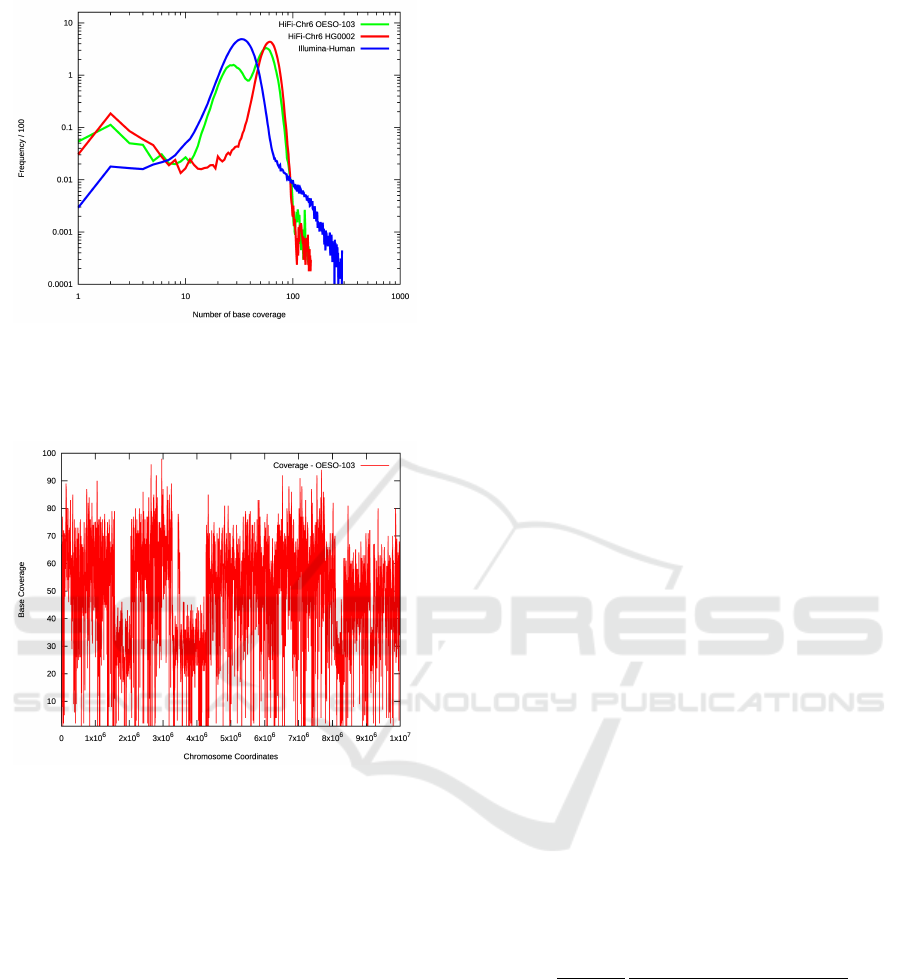
Figure 2: The global coverage distribution of chromosome

6 in the OESO-103 sample, demonstrating a bimodal distri-

bution, with one peak at apporximately half the coverage of

the other, consistent with a change occuring on only one of

a homologous pair.

Figure 3: A snapshot of the per-base coverage of chromo-

some 6 in the OESO-103 sample, showing a marked drop

in coverage around the site of identiﬁed breaks at ∼ 2 ×10

and ∼ 4 × 10

: approximately a drop of one-half, indicat-

ing the presence of two haplotypes generated by one of the

diploid pair having undergone a break/joining at this loca-

tion.

Due to the unusual nature of this particular sam-

ple, it is relatively unambiguous that it is the result of

a chromothripsis process, though we note from Fig-

ures 2 and 3 that there are clear signs from the cov-

erage data that multiple hapolotypes have been gener-

ated - samples which are less extreme might have to

demonstrate more robustly that they are genuinely in

tension with traditional models of cancer formation.

2.3 Future Data

It is evident that the statistical importance of our re-

sults is limited until we can demonstrate that they

hold true across multiple instances of chromothripsis,

rather than just the single case we currently possess.

It is of vital importanance for our future work that

we test these tools on additional chromothripsis sam-

ples. However, as this simply serves as a proof of

concept for the information it is possible to extract,

we continue with our single sample until more data is

available.

3 HYPOTHESISTESTER TOOL

In order to robustly examine models for explaining

the data extracted from our chromothrispis sample,

we must have a statistically robust mechanism for as-

sessing which models are better in explaining the fea-

tures of the data.

We have found the standard statistical tools such

as statistical signiﬁcance testing generally unsuitable

for this task, and thus have joined the chorus (i.e.

(Stang et al., 2010)) of those advocating a Bayesian

approach to model testing and selection.

The primary concern is that, in general, a more

ﬂexible model (i.e. one with more free parameters

which can be ﬁt to the data) will always be able to

provide a better ﬁt than a model with fewer param-

eters, thus, complexity is favoured over simplicity.

As a pathological example, it is always possible to

draw a perfect polynomial ﬁt to N datapoints if the

polynomial is of N − 1

order. If one is faced with

choosing between a straight line which close to (but

not exactly through) 80 data points, or one which

contains terms of order x

but which perfectly goes

through every datapoint, any method which relies

purely on goodness-of-ﬁt would choose the highest-

dimensional model, no matter how ludicrous those

are.

Bayesian tools, however, allow us to directly ac-

cess the relative likelihood between two models, A

and B in explaining the data D, in the form of the

odds-ratio:

Prior(A)

Prior(B)

⃗

λProb



A|D,

⃗



Prior(

⃗

λ)

d⃗µProb(B|D,⃗µ) Prior(⃗µ)

(1)

Here the Prior is the initial belief we have in the

model (and its parameters, µ and λ). If R

≫ 1, then

hypothesis A is much more likely to be true than hy-

pothesis B. Of course, more data might alter this con-

clusion, and Hypothesis C might be better still, but

this provides an objective, numerical way to assess

which model is best.

Although the underlying theory for computing

these odds ratios is available in most introductory

Bayesian Statistics textbooks, the techniques are often

BIOINFORMATICS 2023 - 14th International Conference on Bioinformatics Models, Methods and Algorithms

278

only easily applicable in pathological, simple exam-

ples, and there is remarkably little computational sup-

port enabling widespread use in the non-pathological

cases. To this end, we have developed the ﬂexible

and easy-to-use Bayesian Hypothesis Testing Engine

- HYPOTHESISTESTER - available in both C++ and

Python implementations, which we hope will make

computing odds ratios simple and robust for a wider

audience.

The underlying mechanics of the HYPOTHE-

SISTESTER work and its associated optimisation rou-

tine, AHAB, will be published as (Fraser-Govil and

Boubert, 2023) and (Fraser-Govil, 2023).

4 CHROMOSPA: SIZE AND

POSITION ANALYSIS

Several works (Stephens et al., 2011; Maher and Wil-

son, 2012; Rausch et al., 2012) have noted that the

identiﬁed breakpoints in chromothripsis show signif-

icant clustering - however, this clustering was iden-

tiﬁed as a signal of a “non-random distribution”, a

claim which has since been repeated elsewhere in the

literature (Righolt and Mai, 2012; Korbel and Camp-

bell, 2013; Mardin et al., 2015; Voronina et al., 2020).

However, we note that clustering is emphatically not

a signal of “Non-randomness”, which would imply a

mechanistic, exactly predictable pattern to the break-

points, for which signiﬁcant evidence has not been

demonstrated. Clustering should instead be seen as an

indicator of a bias in the underlying probability dis-

tribution - we must instead interpret the prior use of

“non-random” instead to mean non-globally-uniform.

The location of the breakpoints can give insight

into the underlying distributions which caused the

fracturing of the genome. To this end, we are devel-

oping the CHROMOSPA tool

, which performs statis-

tical analysis on the locations of breakpoints and the

size of the resulting ostracons. This is still a work

in progress, however we discuss brieﬂy some of our

preliminary results.

4.1 Ostracon Size

Once a list of breakpoints has been inferred via STEP-

PINGSTONE, the length of each ostracon can be in-

ferred simply by subtracting successive breakpoint in-

dices from each other: if two neighbouring break-

points on a chromosome are found at i and j respec-

tively, the length of the ostracton is |i − j |.

https://github.com/wtsi-hpag/chromoSPA

0.1

0.2

0.3

0.4

0.5

0.6

0.7

0.8

0.9

1.1

10 10 10 10 10 10 10 10 10

Fractional Fragment Length

Chrom6 observed

Uniform Probability Fit

Figure 4: The observed frequency of ostracon sizes (given

as a fraction of the entire chromosome 6 length) on Chro-

mosome 6 of our sample.

We note that this inference of the ostracon length

assumes that chromothripsis occurs only on a single

copy of (in this case) chromosome 6, since STEP-

PINGSTONE is unable to phase the reads, and hence

cannot distinguish between breakpoints occuring on

different homologous chromosomes. We justify this

by noting in Figs. 2 and 3 that the drop in coverage

of ≈ 50% supports the notion that only one copy of

the chromosome is affected by chromothripsis. How-

ever, future work in this area should make the statis-

tical inference robust against the possibility of multi-

homolog chromothripsis.

Figure 4 shows the observed distribution of the

breakpoints, along with the best-ﬁt probability model,

assuming that breakpoints occur uniformly across the

chromosome. As expected, we see a clear bias of

more smaller ostracons than the uniform model would

predict: this is due to the previously identiﬁed clus-

tering of breakpoints, which produces many smaller

ostracons due to the close proximity of the breaks.

The pattern in Fig. 4 is therefore a superposition

of the length of ostracons within clusters and of the

distance between clusters.

Our analysis shows that the distances between os-

tracons are well explained by a Gaussian mixture

model, such that the probability of a break occuring

at position x is given by:

p(x) =

∑

exp



−

(x − µ

)

2σ



(2)

That is, the probability distribution of each cluster is

(approximately) Gaussian, with σ

≈ 10kb, which re-

sults in osctacon lengths which are in turn distributed

in a Gaussian fashion, with size 5 ± 2kb.

Interestingly, however, we ﬁnd that the distribu-

tion of the focal points of the clusters - the µ

values

Ongoing Work to Study the Underlying Statistical Patterns of Oesophageal Chromothripsis

279

- shows no signiﬁant bias. This is surprising as we

have already identiﬁed several supra-chromosomal

patterns (signiﬁcant chromothripsis only occurs on 1

copy of chromosomes 6 and 9, for example), how-

ever, it seems of those chromosomes which do suffer

chromothripsis, the process results in cluster hotspots

which have no particular positional bias in the chro-

mosome.

This is a tantalising hint that, although the breaks

are highly clustered around the focal points, the dis-

tribution of the focal points is highly random and uni-

form within a chromosome; subject to the chromsome

being a chromothripsis candidate in the ﬁrst place – a

seemingly odd, random process amidst an otherwise

highly ordered heirarchy of events.

We do note, however, that we are limited by our

single chromothripsis sample: comparisons with mul-

tiple samples might reveal that the same positions oc-

cur in multiple events, which would indicate that there

is something special about these locations, but that

this special property is uniformly distributed in the

chromosome.

5 ContactPoint ANALYSIS

In this section we turn to analysing the joinpoints

generated by chromothripsis: studying why a given

ostracon ends up joined to another in the ﬁnal

mignogenome.

One plausible hypothesis is that, after a breakage

occurs, the DNA strands are repaired on the basis of

proximity: once a breakpoint forms, generating an

ostracon with a free end, the joinpoint then prefer-

entially occurs between ostracons which are spatially

close together. Since DNA within the cell forms a

complex 3D structure, the resulting joinpoints when

projected into linear form are then distributed seem-

ingly chaotically and randomly. We dub this hypoth-

esis the ‘Contact Point Hypothesis’.

In order to study this hypothesis, we make one fur-

ther ansatz: namely that the repair process happens

whilst the chromosomes are in their normal spatial ar-

rangement within the cell (i.e. interphase), rather than

during a portion of their lifetime where the chromo-

somes are dramatically repackging themselves. Un-

der this approximation, the spatial mapping is the

same as that extracted from standard HiC techniques

(Lieberman-Aiden et al., 2009).

HiC is a form of Chromatin Conformation Cap-

ture, in which the chromatin strands are crosslinked

with their spatial neighbours, labelled with biotin,

and then excised - producing engineered ’chimeric

reads’, with the chimerism happening preferentially

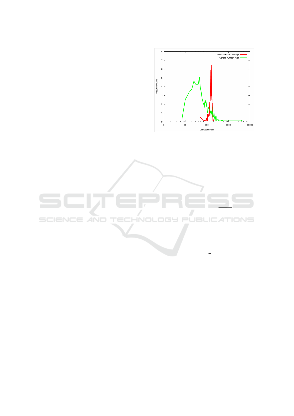
Figure 5: Frequency plots for the values of H

i j

(the contact

number) found at the locations of joinpoints (green), com-

pared to the average value of H

i j

along the corresponding

horizontal of the contact matrix (red).

between reads which are spatially colocated within

the genome. By counting the number of chimerisms

between two regions, one can then build up a HiC

’contact matrix’, H

i j

, which measures how close the

genetic coordinates i and j are in 3D space.

Our hypothesis is equivalent to approximating

that:

Prob(i joins to j) =

i j

∑

i,k

(3)

I.e., the probability of seeing a join at a location is

directly proportional to the HiC contact mapping be-

tween the original ostracon location, and its ﬁnal po-

sition.

Figure 5 demonstrates the distributions of H

i j

ex-

tracted for the joinpoints in our sample, as compared

to the mean value,



i j



∑

i, j

. It seems clear

from this plot that H

i j



i j



almost everywhere,

and hence that the joins are actually occuring very far

away from regions of high contact. It might also be

tempting to take this one step further, and say that the

breakpoints are preferentially happening away from

regions of high contact.

5.1 Additional Complexity: The Need

For A Full Analysis

However, we note that this is a relatively simple anal-

ysis and omits a potentially vitally important corol-

lary: that we potentially do not observe all joinpoints,

and under the Contact Hypothesis, we would actually

expect to not observe the vast majority of joinpoints.

This is because the ContactPoint hypothesis makes no

distinction between a joinpoint and a perfect repair.

BIOINFORMATICS 2023 - 14th International Conference on Bioinformatics Models, Methods and Algorithms

280

If the break was repaired perfectly, we would

have no way to detect that it exists, since we can

only detect joinpoints that result in chimeric align-

ment. Such a break would not be counted by the

green line in Figure 5, despite potentially having

contact counts in the thousands. In short, by the

very nature of the observations, we preferentially

omit our most probable datapoints. The probabil-

ity we need to test is not Prob(join at (i, j)), but

Prob(join at (i, j )||i − j| > X), i.e. the breakpoints

must be far enough apart for them to be distinct and

detectable. There are other additional considerations

to take into account: joins within highly repetitive re-

gions are unlikley to be detected due to the difﬁculty

of accurately aligning to them, for example.

We therefore urge caution in interpreting the raw

data in this fashion, and instead leverage the pow-

erful Bayesian machinery developed in section 3 to

test a number of alternative hypotheses. As noted in

§3, our Bayesian approach is not strictly about ac-

cepting/rejecting a null hypothesis, but about learning

which of a series of proposed models is the best at

describing the data - though we do include a highly

simple model as a pseudo-null, as a baseline against

which all other models are compared.

To this end, we propose three classes of model to

test, corresponding to three basic Hypotheses

1. Hypothesis: There is no pattern: Our null model

(as far as we have one) is the ‘Uniform Weight-

ing’ (UW) model, which assumes that there is

no underlying pattern in the location of the join-

points, and every join is as likely as the others:

i j

= C (4)

This model has no free parameters, as the value of

C is determined by the size of the chromosome.

2. Hypothesis: There is a pattern (but we don’t know

what): The next most simple model assumes that

the chromosome can be split up into N segments:

each segment has a uniform probability of a join

occuring within it, but this varies from segment

to segment: a Multi-Block Uniform Weighting

(MBUW) model.

i j

= A

(

i in block x

j in block y

(5)

This model has N(N + 1)/2 − 1 free parameters,

corresponding to the number of possible A

i j

val-

ues, minus one for the normalisation. We denote

the models with different resolutions as MBUW

3. Hypothesis: The Contact Point Hypothesis is true:

In this case, we use the HiC contact map to gen-

erate a Spatially Associated Weighting (SAW)

model. Since HiC maps are (by nature) sparse,

we pass a Gaussian smoothing kernel of length ℓ

over the map in order to populate all values of p

i j

= smooth



i j

∑

i,k

,ℓ



(6)

We could equally bin the HiC data into coarser

bins, but for the purposes of marginalisation, it

is often more convenient to deal with a continu-

ous parameter. We label the model which has a

smoothing length of 10

bases as SAW

From each of these proposed models for p

i j

, we

are then able to generate a value of P(D|model), the

probability of observing each chromothripsis dataset

(which we recall is a list of join-points (i

, j

) of each

ostracon in detected by STEPPINGSTONE), and hence

compute Eq.(1).

Before testing these models, however, it is use-

ful to ﬁrst discuss what each model being “the best”

would mean. In the case of the SAW model scoring

highly for some reasonable value of ℓ, the conclusion

would be that the Contact Point hypothesis is indeed

a reasonable model for how ostracons are reassem-

beld during chromothripsis. If the UW model scores

highly, it means that all of our proposed models are

less likely than sheer random chance: in this case,

we would probably argue that it is more likely that

we failed to properly formulate a model than the UW

model being ”true” in any meaningful way.

The MBUW models are perhaps the most difﬁ-

cult to interpret; the most obvious point is that if

a MBUW

model is found to outperform both the

UW and SAW models, this implies that there is in-

deed a pattern in the underlying distribution of join-

points, but that it is not the Contact Point hypothe-

sis. However, we can also infer some more informa-

tion, since the MBUW models allow for ﬁne struc-

ture in the probability distribution of the chromosome,

but the so-called ’Occam Factor’ implicit in Eq.(1)

means that arbitrarily high dimensional formulations

are punished. Therefore, if MBUW

is found to be a

good ﬁt, but MBUW

x+1

is not, this implies that the

smallest scale of variation in the underlying pattern

is one-x

of the size of the chromosome. Testing

the MBUW models of arbitrarily high dimension can

therefore be used to infer the variation scale (but can

be computationally very costly due to the multidimen-

sional integrals required: we limit ourselves to x = 25

- a 324 dimensional integral).

Figure 6 shows the results of such an inference on

three classes of model: For each model, we computed

the integral shown in Eq.(1), relative to the best per-

forming model. Note that for ease of interpretation,

we have inverted the scale: a high value means that

the model has performed poorly.

Ongoing Work to Study the Underlying Statistical Patterns of Oesophageal Chromothripsis

281

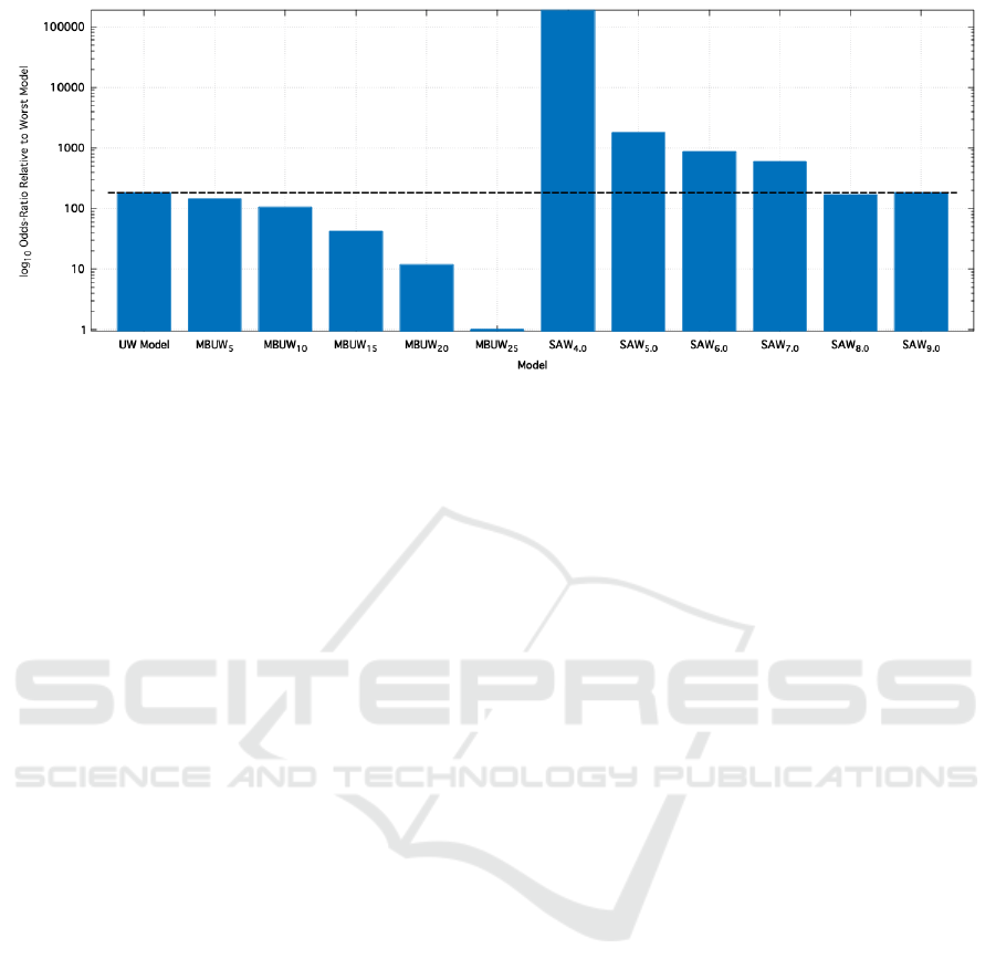
Figure 6: Bayesian inference plot for a number of joinpoint Hypotheses tested against the joinpoint data on chromosome

6 of the OESO-103 dataset. Shown are the values of Eq.(1) computed for each model, normalised such that a value of

x corresponds to a hypothesis 10

x−1

less likely than the most likely one. This demonstrates that even with the additional

considerations detailed in 5.1, the Contact Point hypothesis (detailed by the ‘SAW’ models) provides a signiﬁcantly worse ﬁt

for the data than assuming no underlying pattern at all (the UW model).

Figure 6 clearly shows that the MBUW models

outperform the UW model, which in turn outperforms

almost all the SAW models. It is only by setting the

blurring distance extremely high (non-trivial portions

of the entire chromosome) that the Contact Point hy-

pothesis even approaches the random-pattern of the

UW model.

We therefore conclude that, given this sample

data, the contact point hypothesis in the form pre-

sented is extremely unlikely to be true. However,

there is signiﬁcant indication of underlying patterns

within the position of joinpoints: there is variation in

the probability distribution below the order of 6Mb -

a value determined solely by the computational con-

straints of the 234 dimensional integral.

5.2 The End of Contact Points?

This does not necessarily rule out the notion that join-

points are formed from spatial proximity: it merely

rules out that the spatial mapping is the same as that

measured by HiC data. If the process of chromothrip-

sis occurs during a different phase of chromosome ar-

rangement, then the associated spatial mapping would

also be different: this could be a naturally occuring

rearrangement (i.e. anaphase or apoptosis), or due to

some induced change associated only with the chro-

mothripsis mechanism.

To this end, we are also working on a method to

detect Contact Point association without the need for

the pre-generated map, H

i j

. Under this approach, we

merely have to posit that such a matrix exists, and

then marginalise over all possible mappings, with the

dataset expanded to include multiple chromothripsis

samples. If chromothripsis occurs due to a consistent

spatial mapping, we would therefore ﬁnd a consistent

contact point weighting between the samples.

Of course, in doing so we have no guarantee that

the mapping matrix corresponds to physical proxim-

ity: this would simply demonstrate that there exists a

ﬁxed, underlying mapping between joinpoints across

multiple different instances of chromothripsis, which

is itself an interesting notion.

However, our primary limitation at this time is

a paucity of high quality chromothripsis samples.

Therefore, whilst the statistical machinery is within

reach, we must wait for a larger set of biological sam-

ples.

6 CONCLUSIONS

In this position paper we have detailed a number of

tools and avenues of study that we are developing in

our effort to understand the underlyng statistical prop-

erties of the chromothripsis phenomenon. Although

this is a work in progress and our results only prelim-

inary, we have made great strides in improving our

understanding.

Our HYPOTHESISTESTER tool, though developed

speciﬁcally for this work, has the potential to make

Bayesian statistical inference an easy-to-use and ac-

cessible tool in many diverse and distinct ﬁelds, and

therefore represents a concrete step towards resolv-

ing a particularly strong tension between embattled

camps in the ﬁeld of statistical inference.

We have demonstrated how this tool can be lever-

aged to distinguish between different biological mod-

BIOINFORMATICS 2023 - 14th International Conference on Bioinformatics Models, Methods and Algorithms

282

els, in particular, in the case of the Contact-Point hy-

pothesis, we were able to demonstrate that although

our hypothesis was signiﬁcantly worse than posit-

ing no structure at all, the statistical mechanism un-

derlying HYPOTHESISTESTER clearly indicated that

there is additional structure present, below the scale

of 6Mb: we are able to conﬁrm that there is a statisti-

cal mechanism to be discovered - we are just not quite

sure what it is yet.

In addition, our work on the length of the ostra-

cons generated by the chromothripsis event provided

a glimpse that, although breakpoints undoubtedly ex-

hibit clustering around a series of nexuses, the distri-

bution of these focal points seems to be random and

uniform across chromosome 6, in strong tension with

some claims we have highlighted from the previous

literature. The presence of a uniform distribution of

focal points seems to lie in contradiction to the oth-

erwise highly structured suprachromosomal pattern

(i.e. chromothripsis on only a single copy of a few

chromosomes), and the clustering around these focal

points, a tension which might help inform future stud-

ies into the actual mechanisms of chromothripsis.

We emphasise again that these are some prelim-

inary results, and aknowledge that we must expand

our data beyond the single, unusually proliﬁc case

of chromothripsis we have studied here. We have

also demonstrated several further steps that need to

be taken from a theoretical perspective, in formualt-

ing more robust and powerful statistical models for

both the ostracon size analysis, and the mapless Con-

tact Point testing. However, despite their preliminary

nature, the results here undoubtedly represent an in-

truiging insight into the future work ahead.

ACKNOWLEDGEMENTS

We want to thank Dr Peter Campbell and Dr Jannat

Ijaz, Wellcome Sanger Institute, for providing the oe-

sophageal cancer datasets in the analysis.

REFERENCES

Fraser-Govil, J. (2023). Hypothesis tester: A ﬂexible tool

for bayesian model inference. Unpublished work.

Fraser-Govil, J. and Boubert, D. (2023). An efﬁcient al-

gorithm for stohastic gradient descent on very large

datasets. Unpublished work.

Korbel, J. O. and Campbell, P. J. (2013). Criteria for in-

ference of chromothripsis in cancer genomes. Cell,

152(6):1226–1236.

Lieberman-Aiden, E., Van Berkum, N. L., Williams, L.,

Imakaev, M., Ragoczy, T., Telling, A., Amit, I., La-

joie, B. R., Sabo, P. J., Dorschner, M. O., et al. (2009).

Comprehensive mapping of long-range interactions

reveals folding principles of the human genome. sci-

ence, 326(5950):289–293.

Maher, C. and Wilson, R. (2012). Chromothripsis and hu-

man disease: Piecing together the shattering process.

Cell, 148(1):29–32.

Mardin, B. R., Drainas, A. P., Waszak, S. M., Weis-

chenfeldt, J., Isokane, M., St

utz, A. M., Raeder, B.,

Efthymiopoulos, T., Buccitelli, C., Segura-Wang, M.,

Northcott, P., Pﬁster, S. M., Lichter, P., Ellenberg, J.,

and Korbel, J. O. (2015). A cell-based model sys-

tem links chromothripsis with hyperploidy. Molecular

Systems Biology, 11(9):828.

Rausch, T., Jones, D., Zapatka, M., St

utz, A., Zichner, T.,

Weischenfeldt, J., J

ager, N., Remke, M., Shih, D.,

Northcott, P., Pfaff, E., Tica, J., Wang, Q., Massimi,

L., Witt, H., Bender, S., Pleier, S., Cin, H., Hawkins,

C., Beck, C., von Deimling, A., Hans, V., Brors, B.,

Eils, R., Scheurlen, W., Blake, J., Benes, V., Kulozik,

A., Witt, O., Martin, D., Zhang, C., Porat, R., Merino,

D. M., Wasserman, J., Jabado, N., Fontebasso, A.,

Bullinger, L., R

ucker, F. G., D

ohner, K., D

ohner,

H., Koster, J., Molenaar, J., Versteeg, R., Kool, M.,

Tabori, U., Malkin, D., Korshunov, A., Taylor, M.,

Lichter, P., Pﬁster, S., and Korbel, J. (2012). Genome

sequencing of pediatric medulloblastoma links catas-

trophic dna rearrangements with tp53 mutations. Cell,

148(1):59–71.

Righolt, C. and Mai, S. (2012). Shattered and stitched

chromosomes—chromothripsis and chromoanasyn-

thesis—manifestations of a new chromosome crisis?

Genes, Chromosomes and Cancer, 51(11):975–981.

Solorzano, C. O. S., Pascual-Montano, A., de Diego, A. S.,

Mart

ınez-A, C., and van Wely, K. H. (2013). Chro-

mothripsis: Breakage-fusion-bridge over and over

again. Cell Cycle, 12(13):2016–2023. PMID:

23759584.

Stang, A., Poole, C., and Kuss, O. (2010). The ongoing

tyranny of statistical signiﬁcance testing in biomed-

ical research. European journal of epidemiology,

25(4):225–230.

Stephens, P. J., Greenman, C. D., Fu, B., Yang, F., Bignell,

G. R., Mudie, L. J., Pleasance, E. D., Lau, K. W.,

Beare, D., Stebbings, L. A., McLaren, S., Lin, M.-

L., McBride, D. J., Varela, I., Nik-Zainal, S., Leroy,

C., Jia, M., Menzies, A., Butler, A. P., Teague, J. W.,

Quail, M. A., Burton, J., Swerdlow, H., Carter, N. P.,

Morsberger, L. A., Iacobuzio-Donahue, C., Follows,

G. A., Green, A. R., Flanagan, A. M., Stratton, M. R.,

Futreal, P. A., and Campbell, P. J. (2011). Massive ge-

nomic rearrangement acquired in a single catastrophic

event during cancer development. Cell, 144(1):27–40.

Voronina, N., Wong, J. K., H

ubschmann, D., Hlevnjak, M.,

Uhrig, S., Heilig, C. E., Horak, P., Kreutzfeldt, S.,

Mock, A., Stenzinger, A., et al. (2020). The landscape

of chromothripsis across adult cancer types. Nature

communications, 11(1):1–13.

Ongoing Work to Study the Underlying Statistical Patterns of Oesophageal Chromothripsis

283

REFERENCES

Fraser-Govil, J. (2023). Hypothesis tester: A flexible tool