On Computing Three-Dimensional Camera Motion from Optical Flow
Detected in Two Consecutive Frames
Norio Tagawa
a
and Ming Yang
b
Graduate School of Systems Design, Tokyo Metropolitan University, 6-6 Asahigaoka, Hino, Tokyo, Japan
Keywords:
Camera Motion, Optical Flow, Minimum Variance, Unbiased Estimator, Neyman–Scott Problem.
Abstract:
This study deals with the problem of estimating camera motion from optical flow, which is the motion vector
between consecutive frames. The problem is formulated as a geometric fitting problem using the values of
the depth map as the nuisance parameters. It is a problem whose maximum likelihood estimation does not
satisfy the Cramer–Rao lower bound, and it has long been known as the Neyman–Scott problem. One of the
authors previously proposed an objective function for this problem that, when minimized, yields an estimator
with less variance in the estimation error than that obtained by maximum likelihood estimation. The author
also proposed linear and nonlinear optimization methods for minimizing the objective function. In this paper,
we provide new knowledge on these methods and evaluate their effectiveness by examining methods with low
estimation error and low computational cost in practice.
1 INTRODUCTION
This paper addresses the problem of estimating the
relative three-dimensional (3D) motion between a
camera and the environment from the optical flows
(two-dimensional velocity fields) detected in two con-
secutive frames (Hui and Chung, 2015; Zhu et al.,
2011). In recent years, many problems in computer
vision have been effectively solved by deep learn-
ing methods, and their performance has been reported
to significantly exceed that of conventional computa-
tional approaches. Deep learning models and meth-
ods for optical flow detection, 3D reconstruction of
the environment based on optical-flow analysis, and
the detection of moving objects have been investi-
gated using both supervised and unsupervised learn-
ing methods (Zhu et al., 2011; Stone et al., 2021; Jon-
schkowsk et al., 2020; Ranjan et al., 2019; Yin and
Shi, 2018).
By contrast, in the field of computational neuro-
science, the existence of a neural system that outputs
the solution to the equations of motion has been con-
firmed in human brain functions such as action de-
cisions based on the perception of the environment
(Piloto et al., 2022; Chen et al., 2022). The equa-
tions of motion are derived by humans from a meta-
perspective based on the analysis of phenomena, and
the brain learns these equations through experience
a
https://orcid.org/0000-0003-0212-9265
b
https://orcid.org/0000-0001-8413-5735
and outputs the solutions in an analog manner using
neural networks. This can be interpreted as mean-
ing that the phenomena occurring in the human brain
can be expressed by mathematical equations as a phe-
nomenon in the natural world.
Considering the above, deep learning is highly ef-
fective for pure pattern recognition problems that are
difficult to solve algebraically or analytically, such
as visual or acoustic recognition. For pure pattern
recognition problems where it is difficult to determine
which features are effective, i.e., problems that are
difficult to solve algebraically or analytically, deep
learning is likely to be very powerful. By contrast, for
tasks that are more mathematical in nature, i.e., tasks
that can be analyzed computationally by humans from
a meta-perspective, it would be more efficient to teach
the necessary mathematical expressions to the com-
puter rather than to learn (derive) them from the data.
Since not all of the same tasks can be described com-
pletely in terms of mathematical formulas, the appli-
cation of a neural network learning function for the
parts that cannot be solved computationally should
also be considered.
From this standpoint, this paper considers the es-
timation of camera motion as a computational ap-
proach. This problem is generally called a fitting
problem, and the basic equation is a fitting equation
of the following form, where Θ is the parameter to be
determined:
a
⊤
i
(Θ)c
0
i
+ b
i
(Θ) = 0, (1)
Tagawa, N. and Yang, M.
On Computing Three-Dimensional Camera Motion from Optical Flow Detected in Two Consecutive Frames.
DOI: 10.5220/0011785300003417
In Proceedings of the 18th International Joint Conference on Computer Vision, Imaging and Computer Graphics Theory and Applications (VISIGRAPP 2023) - Volume 5: VISAPP, pages
931-942
ISBN: 978-989-758-634-7; ISSN: 2184-4321
Copyright
c
 2023 by SCITEPRESS – Science and Technology Publications, Lda. Under CC license (CC BY-NC-ND 4.0)
931

where a
i
(Θ) is a vector function independent of the
observables, b
i
(Θ) is a scalar function independent
of the observables, and c
i
is a vector consisting of
parameter-independent observables. In addition, c
0
i
means that the observation is error free. Since c
i
usu-
ally contains observation noise, the solution Θ
0
does
not completely satisfy Eq. 1. Therefore, we are left
to solve the following minimization problem for the
objective function, where N is the number of observa-
tions:
J(Θ) =
N
∑
i=1
n
a
⊤
i
(Θ)c
i
+ b
i
(Θ)
o
2
. (2)
Maximum likelihood estimation is based on the ob-
servation equations that model the observables. The
fitting equations can be rewritten into the observa-
tion equations, which require an additional unknown
quantity that increases with the number of observa-
tions, called the latent parameter or nuisance param-
eter. The maximum likelihood estimator (MLE) gen-
erally achieves the Cramer–Rao lower bound (CRLB)
asymptotically. However, in the fitting problem, the
variance of the MLE is larger than the CRLB because
of the effect of this nuisance parameter. This has been
known for a long time as the Neyman–Scott problem
(Bickel et al., 1993). Furthermore, it has been shown
through our previous study (Tagawa et al., 1993) that
the estimator that minimizes Eq. 2 is biased if the
following equation, where the noise component of
the observation c
i
is denoted by δc
i
and the expected
value operation by E[·] does not hold:
N
∑
i=1
a
⊤
i
(Θ)E
h
δc
i
δc
⊤
i
i
a
i
(Θ) = Constant. (3)
The estimation of camera motion from optical flow
corresponds to this.
We have shown that by introducing appropriate
weights to each observation in Eq. 2, it is possible
to construct an objective function to asymptotically
eliminate the bias of the above estimators and to bring
the variance of the estimators close to the CRLB.
Moreover, we have constructed its minimization al-
gorithm (Tagawa et al., 1994a; Tagawa et al., 1994b;
Tagawa et al., 1996). However, we have only theoret-
ically clarified the possibility of the existence of such
superior weights and provided some specific exam-
ples. In this paper, we first give a new interpretation
of this minimization algorithm. Then, based on this
interpretation, we discuss weight determination meth-
ods to bring the variance of the estimator closer to the
CRLB.
The main contributions of this study can be sum-
marized as follows.
• We give a new interpretation of the linear method,
which is an efficient estimation method for cam-
era motion approximated by infinitesimal motion.
• In the unbiased and efficient minimizable
weighted objective function we proposed for
camera motion estimation, we specifically con-
struct a weight function that reduces the variance
of the estimator to that of the MLE, and evaluate
its effectiveness in detail. In the process, we also
clarify the influence of the characteristics of the
linear method described above.
The rest of this paper is organized as follows: we
first briefly mention related works in Sec. 2. We then
explain our proposed unbiased objective function and
present our new findings on it in Sec. 3. In Sec. 4, we
make a practical proposal for the weight function that
appears in the objective function described in Sec. 3
and show the effectiveness of the estimator based on
it. The results obtained in this study are discussed in
Sec. 5 and conclusions are presented in Sec. 6.
2 RELATED WORKS
Another method for reducing the variance of the esti-
mator is an empirical Bayesian approach that uses the
prior probability of the nuisance parameters (Maritz,
2018; Huang, 2019; Yuille and Kersten, 2006). How-
ever, there is a risk that model deviations in the prior
probabilities may lead to biased estimators. By con-
trast, the weighted least squares method used in this
study does not cause bias in the estimator, no matter
what the weights are. Therefore, it is possible to uti-
lize prior knowledge of the nuisance parameters while
maintaining unbiasedness, which is a major feature of
our method.
If the probability distribution shape of the depth is
known, i.e., the above mentioned bias does not occur,
the variance of the camera motion estimation by the
empirical Bayesian method reaches the CRLB. This
CRLB is the lower bound as an average over the var-
ious depths. In order to compare this with the CRLB
in the non-parametric setting in which the depth is a
definite unknown in this study, the latter must be aver-
aged with respect to the depth. And due to the amount
of probabilistic information, the CRLB for empirical
Bayes is expected to be lower than that.
However, in practical applications, the object
or environment to be imaged changes over time,
and thus the probability distribution shape of depth
also changes. In visual simultaneous localization
and mapping (visual SLAM) (Tateno et al., 2017;
Sumikura et al., 2019; Chaplot et al., 2020), although
VISAPP 2023 - 18th International Conference on Computer Vision Theory and Applications
932

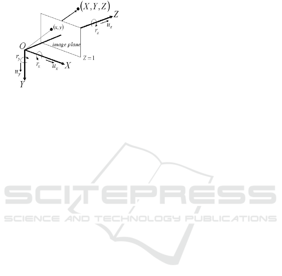
Figure 1: Camera projection model and notation definition.
an accurate model of the 3D environment is con-
structed by adjusting bundles for many frames, it is
important to know the exact camera position and ori-
entation at each instant. In these cases, a reliable esti-
mate for each depth is considered more effective than
a good estimate in an average sense. Originately, the
assumption that all depth probability distributions are
known is not realistic.
3 OBJECTIVE FUNCTION FOR
CAMERA MOTION
In this section, we refer to our previously proposed
objective function for camera motion estimation. In
Sec. 3.1, we show that the epipolar equation defined
for the infinitesimal motion of the camera is an in-
finitesimal approximation of that equation for finite
motion. In Sec. 3.2, we derive a new interpretation
of the efficient estimation method, called the linear
method, obtained on the basis of the infinitesimal
epipolar equation. In Sec. 3.3, as a preparation for
the next section, we outline our weighted objective
function, which allows unbiased and low variance es-
timation with low computational complexity.
3.1 Infinitesimal Epipolar Equation
Let (X ,Y, Z) be a camera coordinate system whose
origin is the lens center. The image plane is defined as
k
⊤
[X,Y,Z] = 1. Vector k is a unit vector perpendicular
to the image plane, and the vertical distance between
the lens center and the image plane is 1. In this case,
the perspective projection of a point X
i
in 3D space
onto the image plane is x
i
= X
i
/k
⊤
X
i
.
A camera moves with a translational velocity vec-
tor u = [u
x
,u
y
,u
z
]
⊤
and a rotational velocity vector
r = [r
x
,r
y
,r
z
]
⊤
relative to the environment. At this
time, the optical flow v
0
i
on the image plane is given
by
v
0
i
= −v
r
i
(r) −d
i
v
u
i
(u), (4)
v
u
i
(u) ≡ Φ
i
u, (5)
v
r
i
(r) ≡ Φ
i
(r ×x
i
), (6)
Φ
i
≡ I −x
i
k
⊤
. (7)
Here, a ×b is the outer product of vectors a, and b
and d
i
= 1/Z
i
is called shallowness. Since d
i
and u
take the product form, their scales are not uniquely
determined. In the following, the magnitude of u is
set to 1 and treated as a unknown with two degrees of
freedom.
Define a
i
(u) ≡u ×x
i
and take the inner product of
this and both sides of Eq. 4.
a
i
(u)
⊤
v
0
i
= −a
i
(u)
⊤
v
r
i
(r) −d
i
a
i
(u)
⊤
v
u
i
(u). (8)
On the right-hand side of the above equation, both u
and x
i
are perpendicular to a
i
(u), yielding the follow-
ing equation without d
i
.
a
i
(u)
⊤
v
0
i
+ a
i
(u)
⊤
(r ×x
i
) = 0. (9)
This is the epipolar equation for infinitesimal motion.
The epipolar equation for finite motion is ex-
pressed as follows for the corresponding points at two
viewpoints (x, x + δx).
(x + δx)
⊤
Ex = 0. (10)
For finite motion, Ex = (t ×R)x using the translation
vector t and the rotation matrix R. For infinitesimal
motion, we can write Rx = x + r ×x as an approxi-
mation, so the operator corresponding to the essential
matrix E for finite motion is given by
E = (u×) + (u ×r×). (11)
Transforming Eq. 10 using this expression yields
x
⊤
(u ×x) + x
⊤
(u ×(r ×x))+ δx
⊤
(u ×x)
+δx
⊤
(u ×(r ×x)) = 0. (12)
The first term is zero, and the fourth term is an in-
finitesimal of the third order, and hence we omit it.
Then, replacing δx by v
0
, we obtain
(u ×x)
⊤
v
0
+ x
⊤
(u ×(r ×x)) = 0. (13)
The following procedure shows that this is equal to
Eq. 9. The second term of Eq. 9 can be transformed
as follows:
a
i
(u)
⊤
(r ×x) = (u
⊤
r)(x
⊤
x) −(u
⊤
x)(x
⊤
r). (14)
By contrast, the vector triple product of the second
term in Eq. 13 can be expanded as follows:
u ×(r ×x) = (u
⊤
x)r −(u
⊤
r)x. (15)
From the above, we see that the second term in Eq. 9
is equal to the second term in Eq. 13.
On Computing Three-Dimensional Camera Motion from Optical Flow Detected in Two Consecutive Frames
933

3.2 New Interpretation of the Linear
Method for the Least-Squares
Objective Function
The epipolar equation in Eq. 9 does not hold if the
observed optical flow v
i
contains errors. Therefore, it
is natural to consider minimizing the sum of squares
of the left-hand side. To prepare for this, the left-
hand side of the epipolar equation (Eq. 9) transforms
a
i
(u)
⊤
v
i
+ a
i
(u)
⊤
(r ×x
i
) as follows:
a
i
(u)
⊤
v
i
+ a
i
(u)
⊤
(r ×x
i
)
= (u ×x
i
)
⊤
v
i
+ (u ×x
i
)
⊤
(r ×x
i
)
= (x
i
×v
i
)
⊤
u + (u
⊤
r)(x
⊤
i
x
i
) −(u
⊤
x
i
)(x
⊤
i
r)
= (x
i
×v
i
)
⊤
u + ∥x
i
∥
2
r
⊤

I −
x
i
x
⊤
i
∥x
i
∥
2

u
= (x
i
×v
i
)
⊤
u + r
⊤
P
i
u
= m
i
(r)
⊤
u, (16)
m
i
(r) ≡ x
i
×v
i
+ P
i
r, (17)
where P
i
≡ ∥x
i
∥
2
−x
i
x
⊤
i
. Using this representation,
we define the least-squares objective function based
on the epipolar equation as follows:
J
LS
(u,r) =
N
∑
i=1
u
⊤
m
i
(r)m
i
(r)
⊤
u
= u
⊤
N
∑
i=1
m
i
(r)m
i
(r)
⊤
!
u
= u
⊤
M(r)u, (18)
where N is the number of observed pixels.
Equation 18 is a nonlinear function with respect
to u and r, and its minimization requires nonlinear
optimization, and hence good initial values are de-
sired. By contrast, for camera motion estimation us-
ing the epipolar equation for finite motion, there is
an efficient computational method called the 8-point
method or linear method (Tagawa et al., 1993). The
same method is applicable to the infinitesimal epipo-
lar equation. In the following, we explain a new inter-
pretation of the method.
In Eq. 16, r
⊤
P
i
u = u
⊤
P
i
r, r
⊤
P
i
u = tr(ur
⊤
P
i
), and
u
⊤
P
i
r = tr(ru
⊤
P
i
), where trA is the trace of matrix A.
Hence, the following equation holds.
r
⊤
P
i
u =
1
2
n
tr(ur
⊤
P
i
) + tr(ru
⊤
P
i
)
o
= tr

1
2
(ur
⊤
+ ru
⊤
)P
i

= ⟨E,P
i
⟩, (19)
E ≡
1
2
(ur
⊤
+ ru
⊤
), (20)
where ⟨A,B⟩ denotes the Frobenius inner product of
the matrices. Using Eq. 19, J
LS
in Eq. 18 can be ex-
pressed as
J
LS
(u,r) =
N
∑
i=1
|(x
i
×v
i
)
⊤
u + ⟨E,P
i
⟩|
2
. (21)
Matrices P
i
and E are symmetric matrices and have
six independent components. Therefore, we define
the following 6-dimensional vectors.
c
i
≡
[P
i(1,1)
,P
i(2,2)
,P
i(3,3)
,
√
2P
i(1,2)
,
√
2P
i(1,3)
,
√
2P
i(2,3)
]
⊤
,
(22)
e ≡
[E
(1,1)
,E
(2,2)
,E
(3,3)
,
√
2E
(1,2)
,
√
2E
(1,3)
,
√
2E
(2,3)
]
⊤
.
(23)
Using these vectors, J
LS
can be further transformed as
follows:
J
LS
(u,r) = u
⊤
Au + 2e
⊤
Bu + e
⊤
Ce, (24)
A ≡
N
∑
i=1
(x
i
×v
i
)(x
i
×v
i
)
⊤
, (25)
B ≡
N
∑
i=1
c
i
(x
i
×v
i
)
⊤
, (26)
C ≡
N
∑
i=1
c
i
c
⊤
i
. (27)
In the following, we derive a linear method based
on Eq. 24. We define a 9-dimensional vector s
i
con-
sisting of observables including pixel positions and a
9-dimensional vector p of unknowns.
s
i
≡ [c
⊤
i
,(x
i
×v
i
)
⊤
]
⊤
, (28)
p ≡ [e
⊤
,u
⊤
]
⊤
. (29)
Using these, Eq. 24 can be written as
J
LS
(u,r) = p
⊤
N
∑
i=1
s
i
s
⊤
i
!
p
= p
⊤
[s
1
,s
2
,··· ,s
N
]





s
⊤
1
s
⊤
2
.
.
.
s
⊤
N





p. (30)
The matrix consisting of s
i
is rewritten as
S
⊤
≡





s
⊤
1
s
⊤
2
.
.
.
s
⊤
N





= [t
1
,t
2
,··· ,t
9
] ≡ T . (31)
VISAPP 2023 - 18th International Conference on Computer Vision Theory and Applications
934

Here, {t
i
} are each bivariate functions on the im-
age plane, and from Eqs. 22 and 28, {t
1
,t
2
,··· ,t
6
}
are functions of second degree or lower. It can also
be seen that these functions are linearly independent,
except when the optical flow is only observed as a
quadratic curve on the image plane. By contrast, from
Eq. 28, {t
7
,t
8
,t
9
} contain {v
i
} and hence have terms
of degree three or higher, unless the object has a spe-
cial shape such as a plane. Therefore, we extract the
projection components from {t
7
,t
8
,t
9
} to the space
with {t
1
,t
2
,··· ,t
6
} as a basis.
[t
1
,t
2
,··· ,t
6
]










t
⊤
1
t
⊤
2
.
.
.
t
⊤
6





[t
1
,t
2
,··· ,t
6
]





−1
×





t
⊤
1
t
⊤
2
.
.
.
t
⊤
6





[t
7
,t
8
,t
9
]
= [t
1
,t
2
,··· ,t
6
]C
−1





t
⊤
1
t
⊤
2
.
.
.
t
⊤
6





[t
7
,t
8
,t
9
] (32)
Thus, the matrix corresponding to B in Eq. 24 with
functions of the second degree or lower is given by





t
⊤
1
t
⊤
2
.
.
.
t
⊤
6





[t
1
,t
2
,··· ,t
6
]C
−1





t
⊤
1
t
⊤
2
.
.
.
t
⊤
6





[t
7
,t
8
,t
9
]
=





t
⊤
1
t
⊤
2
.
.
.
t
⊤
6





[t
7
,t
8
,t
9
]. (33)
This is consistent with B. Similarly, the matrix cor-
responding to A in Eq. 24 can be obtained by multi-
plying the transpose matrix of Eq. 32 by itself from
the left: B
⊤
C
−1
B. To summarize the above, Eq. 24,
or Eq. 30, can be separated into terms based on func-
tions of the second degree or lower and terms based
on functions of the third degree or higher, as follows:
J
LS
(u,r) = p
⊤

C B
B
⊤
B
⊤
C
−1
B

p
+p
⊤

0 0
0 −B
⊤
C
−1
B + A

p. (34)
The first term can be further decomposed as follows:
J
low
LS
(u,r) ≡ e
⊤
Ce + 2e
⊤
Bu + u
⊤
B
⊤
C
−1
Bu. (35)
Similarly, the second term can be written as
J
high
LS
(u) ≡ u
⊤

A −B
⊤
C
−1
B

u. (36)
Minimizing J
high
LS
(u) with respect to u corresponds to
the linear method.
The eigenvector corresponding to the smallest
eigenvalue in the following eigenvalue problem is the
solution ˆu by the linear method:

A −B
⊤
C
−1
B

u = λu. (37)
Information on r is contained only in Eq. 35 and must
be minimized. Since this requires nonlinear optimiza-
tion, the linear method treats e as a variable indepen-
dent of u (an expansion of the solution space), and
then determines e as
ˆe = −C
−1
Bˆu. (38)
Then, multiplying by ˆu from the right side of Eq. 20,
the following equation is obtained.
ˆ
E ˆu =
1
2

I + ˆuˆu
⊤

r (39)
Here, using (I + ˆuˆu
⊤
)
−1
= I −(1/2)ˆuˆu
⊤
, r can be ob-
tained by the following equation:
ˆr = 2

I −
1
2
ˆuˆu
⊤

ˆ
E ˆu. (40)
3.3 Objective Function for Unbiased
and Low Variance Estimation
The solution that minimizes the objective function of
Eq. 30 is generally biased. Furthermore, since the
epipolar equation s
⊤
i
p = 0 is a fitting equation and in-
cludes the depth inverse {d
i
}, which is a nuisance pa-
rameter, the variance of the obtained estimator does
not reach the CRLB. That is, the estimator does not
have asymptotic efficiency. An objective function that
allows asymptotically unbiased estimation with less
variance has therefore been proposed (Tagawa et al.,
1994b; Tagawa et al., 1996). Using the notation of
Eq. 18, the objective function, which is a generalized
quotient unbiased objective function, is expressed as
follows:
J
GQU B
(u,r) ≡
u
⊤

∑
N
i=1
∑
N
j=1
λ
i j
m
i
(r)m
j
(r)
⊤

u
u
⊤

∑
N
i=1
λ
ii
Γ
i

u
,
(41)
Γ
i
≡ Φ
⊤
i
Φ
i
. (42)
The N ×N matrix Λ with λ
i j
elements is a positive
definite weight matrix. Equation 41 can be expressed
On Computing Three-Dimensional Camera Motion from Optical Flow Detected in Two Consecutive Frames
935

in terms of its numerator in the notation of Eq. 30 as
follows:
J
GQU B
(u,r) =
p
⊤
T
⊤
ΛT p
u
⊤

∑
N
i=1
λ
ii
Γ
i

u
. (43)
Furthermore, using the notation of Eq. 21, we obtain
the following expression:
J
GQU B
(u,r) =
u
⊤
A
Λ
u + 2e
⊤
B
Λ
u + e
⊤
C
Λ
e
u
⊤

∑
N
i=1
λ
ii
Γ
i

u
. (44)
Each matrix in the numerator is defined as a submatrix
of the matrix vecT
⊤
ΛT as follows:
T
⊤
ΛT ≡

C
Λ
B
Λ
B
⊤
Λ
A
Λ

. (45)
The objective function has a sum operation on the pix-
els in the denominator and numerator, respectively.
This significantly reduces the computational com-
plexity when iterating through nonlinear optimiza-
tion. In contrast, the objective function for MLE is
computationally expensive because the rational func-
tion is included in the summation operation (Tagawa
et al., 1994a)
For the estimator obtained using the weight ma-
trix Λ, see Eq. 51 in the appendix. The appendix also
shows the general form of the variance-covariance
matrix of the estimator for the weights Λ (Eq. 51),
the optimal weights Λ
opt
(Eq. 52), and the variance-
covariance matrix for them (Eq. 53). We also
define a quasi-optimal weight matrix Λ
F
≡ P
F
5
=
F(F
⊤
F)
−1
F
⊤
as a projection matrix. However, since
both weight matrices require a true value of the pa-
rameter Θ
0
, they cannot be applied as is.
Let us summarize our findings on weight matri-
ces. To reduce the σ
2
term, a projective matrix con-
taining the space S
F
spanned by five column vectors
of F is desirable. The I
N
are the simplest weights that
satisfy this condition. By contrast, to reduce the σ
4
term, the dimension of the projective space should be
small. If the dimensions of the projective space are
reduced, S
F
is not sufficiently included, and thus the
σ
2
term becomes larger while the σ
4
term becomes
smaller. When the dimensions of the projective space
are increased, just the opposite phenomenon occurs.
4 WEIGHT MATRIX FOR LOW
VARIANCE ESTIMATION
In this section, we refer to the weight function in the
objective function described in Sec. 3.3. In Sec. 4.1,
we show that the theoretical optimal weights shown
in the appendix do not yield a solution by the linear
method. In Sec. 4.2, we discuss a practical weight
function to reduce the variance of the estimator. In
Sec. 4.3, we evaluate numerically the effect of the
weight function.
4.1 Weights for the Unbiased Linear
Method
The generalized quotient unbiased objective function
is nonlinear with respect to Θ, and a numerical iter-
ative method based on the perturbation principle of
eigenvalues is an effective method for its minimiza-
tion. To avoid local solutions, iterations from initial
values close to the true value are desirable. The linear
method described in Sec. 3.2 is one candidate. Based
on the discussion in Sec. 3.3, the objective function
for the unbiased linear method is a modification of
Eq. 36 as follows:
J
high
GQU B
(u) ≡
u
⊤

A
Λ
−B
⊤
Λ
C
−1
Λ
B
Λ

u
u
⊤

∑
N
i=1
λ
ii
Γ
i

u
. (46)
Consider the case where Λ = Λ
opt
. Since D is
of full rank, rankF = 6, and from the definition of
Eq. 52, the rank of Λ
opt
is five. In Eq. 45, rankT = 9,
except for special cases such as quadric surfaces.
Therefore, rank(T
⊤
ΛT ) = 5 holds. This means that
only five degrees of freedom can be determined by
minimizing Eq. 41. In addition, it can be seen that
there is no inverse of C
Λopt
, which is a 6 ×6 matrix.
Therefore, Eq. 46 cannot be defined, and the unbiased
linear method with optimal weights cannot be used.
Note that ˆu can be computed by defining the numera-
tor of Eq. 46 as u
⊤
A
ΛOPT
u. This is because the matrix
in the numerator of Eq. 41 can be decomposed as fol-
lows:
T
⊤
ΛT =

C
Λ
B
Λ
B
⊤
Λ
0

+

0 0
0 A
Λ

, (47)
and in the absence of noise, both quadratic forms must
be zero. However, subsequent calculations of the lin-
ear method (from Eq. 38 to Eq. 40) are not possible.
The above is the case when Λ
opt
is used, but by
the same consideration, it is clear that the unbiased
linear method cannot obtain a unique solution with-
out using a rankΛ ≥ 8 weight matrix. This is due to
the fact that the (unbiased) linear method extends the
solution space to eight dimensions. In the unbiased
linear method, the objective function to be minimized
is J
GQU B
without the second-order or lower polyno-
mial function component, and hence it is desirable to
take advantage of sufficient information by projecting
to a functional subspace with many polynomial func-
tions of third order or higher as the basis.
VISAPP 2023 - 18th International Conference on Computer Vision Theory and Applications
936

4.2 Weights as a Superior Projection
Matrix
Unlike unbiased linear methods, in the minimization
of J
GQU B
, i.e., nonlinear optimization, the projection
matrix to a low-dimensional functional subspace con-
taining optical flow, which is a two-dimensional vec-
tor function, is desirable as weights, according to
Sec. 3.3’s argument. Depth, and thus optical flow, is
generally smooth, except for some areas such as the
edges of objects. Therefore, we can define several
bivariate functions, each of which supports a locally
connected region where the depth does not change
significantly. The projection matrices to the subspace
created by these functions can be used as weights.
As an example, this idea can be realized by divid-
ing the image into small connected regions and deter-
mining the weights as in the following equation.
λ
i j
= 1/N
i j
(i and j are in the same region),
= 0 (i and j are not in the same region).
(48)
The weights are projection matrices into the subspace
spanned by M bivariate functions, each defined for
each subdomain. The complexity of Eq. 45 with these
weights is O(N), independent of M, and is obtained
at low computational cost. In particular, the adop-
tion of connected regions leads to the definition of
smooth function groups, which are suitable for ap-
proximating optical flows. As the number of regions
is increased, more local functions tend to be em-
ployed, and the higher-order polynomial component
increases. The weights can also be interpreted as av-
eraging the epipolar equations of pixels in the same
subregion without distinction.
4.3 Evaluation
To verify the effect of the projection matrix type
weights described in the previous section, we employ
a simple method of dividing the image into dice-like
rectangular regions. Then, additive noise is added to
the theoretically obtained optical flow, camera motion
estimation is performed using it as an observation,
and its accuracy is evaluated numerically.
Consider an object consisting of multiple planes
as the imaging target, and consider two images of
the object taken by the camera under minute transla-
tions and rotations. Using the camera motion and the
depth map, the theoretical value of the optical flow
is calculated from Eq. 4. Figure 2 shows the three
depth maps used in this experiment, each with a dif-
ferent number of constituent planes. An image of
120 ×120 pixels was defined with an angle of view
(a) (b)
(c)
Figure 2: Depth maps consisting of the planes used in the
simulation, with (a) low, (c) high, and (b) intermediate num-
bers of planes.
whose height and width are equal to the focal length.
The depth Z(x,y) is measured with respect to the fo-
cal length, where the furthest distance is 15 and the
standard deviation of convexity toward the camera at
that point is 10. The translation velocity vector of the
camera is u = [0.4, 0.0,0.2]
⊤
, the rotation vector is
r = [0.04,−0.02, 0.0]
⊤
, and the average length of the
optical flow vector is a few pixels.
Since the length of the translation vector cannot
be estimated, the root mean squared error (RMSE)
between the estimated value obtained as a unit vec-
tor and the set value of the translation vector con-
verted to a unit vector was evaluated. Figures 3–5
show the RMSE (vertical axis) versus the number of
image divisions (horizontal axis), which determines
the weight function. In this study, the weight func-
tion is defined by dividing the image into square re-
gions, and hence the number of divisions is the value
for both the x and y axes of the image. Figures 3, 4,
and 5 correspond to the results for the depth maps in
Figure 2(a), (b), and (c), respectively. In each figure,
(a) shows the results obtained by the linear method
and (b) shows the results obtained by nonlinear opti-
mization. The added noise follows a white Gaussian
distribution, and its standard deviation varies as a ra-
tio of the mean optical flow length. The ratio is varied
in eight different ways, from 0.02 to 0.30, as a param-
eter of the graph.
These results show, first, that as the spatial distri-
bution of the depth becomes more complex, the error
is minimized in a greater number of divided regions.
Namely, the results confirm the hypothesis that a pro-
jection matrix that adequately approximates the opti-
cal flow (a bivariate function) but has a low dimen-
On Computing Three-Dimensional Camera Motion from Optical Flow Detected in Two Consecutive Frames
937

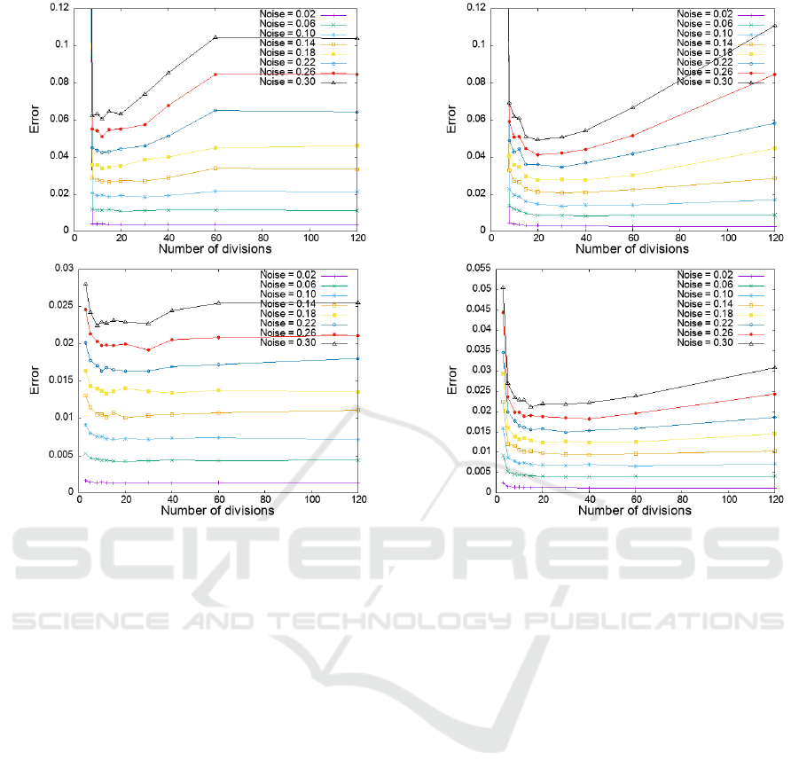
(a)
(b)
Figure 3: Variation of the estimation error of the camera
translation velocity vector for the depth map in Fig. 2(a) de-
pending on the number of region divisions determining the
weight function: (a) linear method, (b) nonlinear optimiza-
tion.
sionality is desirable as a weight function for the gen-
eralized quotient unbiased objective function. It was
also shown that for any depth map, a weight function
with an appropriate number of divisions provides a
better estimation than no weight, since 120 divisions
corresponds to no weights, i.e., the unit matrix is used
as the weight. The above holds true for both linear
and nonlinear optimization. Comparing (a) and (b)
in each figure, we can see that the error in the lin-
ear method is about four times worse than that of the
nonlinear optimization in all cases. It can also be
seen that for every depth map, the linear method has a
larger number of appropriate divisions. This is a con-
sequence of the fact that the linear method uses only
the higher-order components of the optical flow for
estimation, as discussed in Sec. 4.2 More importantly,
we find that nonlinear optimization yields approxi-
mately the same estimation accuracy regardless of the
complexity of the depth map using a weight function
based on the appropriate number of divisions.
The estimation error obtained from the nonlinear
optimization was then replotted against the magnitude
of the optical flow noise in Fig. 6. This figure shows
(a)
(b)
Figure 4: Variation of the estimation error of the camera
translation velocity vector for the depth map in Fig. 2(b)
depending on the number of region divisions determining
the weight function: (a) linear method, (b) nonlinear opti-
mization.
the results using the optimal weight function, the re-
sults from MLE, and the results using a weight func-
tion based on various numbers of region divisions.
Figure 6(a), (b), and (c) show the results for the depth
maps in Fig. 2(a), Fig. 2(b), and Fig. 2(c), respec-
tively. The first thing we see is that the estimation
obtained by the optimal weight function is the best for
any depth map, i.e., independent of the spatial com-
plexity of the depths. Furthermore, a better estima-
tion than MLE can be achieved using a weight func-
tion with an appropriate number of region divisions. It
should be emphasized that estimation with all weight
functions is superior to MLE when the depth is less
uneven and the optical flow noise is higher.
5 DISCUSSIONS
The method of determining the appropriate number
of region divisions for weight determination is an im-
portant issue for the future. In addition, although
we employed a fixed-size rectangle in this study, we
should be able to obtain a more effective determi-
VISAPP 2023 - 18th International Conference on Computer Vision Theory and Applications
938

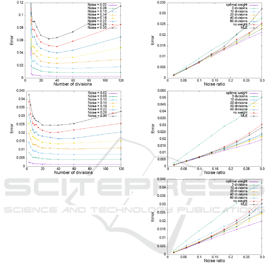
(a)
(b)
Figure 5: Variation of the estimation error of the camera
translation velocity vector for the depth map in Fig. 2(c) de-
pending on the number of region divisions determining the
weight function: (a) linear method, (b) nonlinear optimiza-
tion.
nation of the weight function if the rectangle size is
also determined adaptively. The above can be easily
achieved if the statistics of the optical flow noise are
known. To determine the variance in the optical flow
noise, for example, the entire problem can be formu-
lated within the framework of a variational Bayesian
method (Sroubek et al., 2016; Sekkati and Mitiche,
2007). Thereby, the variance of the optical flow noise
can be estimated by an empirical Bayesian method
(Tagawa, 2010).
Achieving the optimal weight function in Eq. 52
is also an issue for further study. Although the true
camera motion and depth map cannot be known, it is
possible to construct the approximate optimal weights
using those estimates. By iteratively repeating the
procedure, we can expect to eventually achieve a good
estimation once the procedure converges. Since depth
has many degrees of freedom, its treatment is an im-
portant technical factor, and maximum a priori esti-
mation could also be applied.
We proposed an MLE algorithm of depth and
camera motion for two consecutive frames in the
framework of multi-resolution processing (Tagawa
(a)
(b)
(c)
Figure 6: Relationship of the estimation error of the camera
translation velocity vector obtained by nonlinear optimiza-
tion to optical flow noise: (a), (b), and (c) results for the
depth maps in Figs. 2(a), 2(b), and 2(c), respectively.
et al., 2008; Tagawa and Naganuma, 2009). The algo-
rithm consists of a Bayesian network in the resolution
direction and propagates the depth and camera mo-
tion information obtained from the low-resolution im-
age to the high-resolution processing, thereby avoid-
ing aliasing and maintaining discontinuity in the op-
tical flow analysis. As shown in Fig. 7, in the low-
resolution layer, the depth is assumed to be con-
stant for each block in the image, and the mean and
variance of the depth posterior probability estimated
there are propagated to the blocks in the upper resolu-
On Computing Three-Dimensional Camera Motion from Optical Flow Detected in Two Consecutive Frames
939

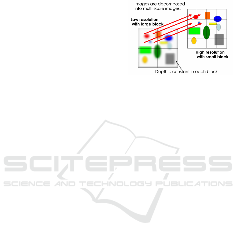
tion layer, which are narrower than those in the low-
resolution layer. To improve the accuracy of camera
motion estimation, a scheme using a generalized quo-
tient unbiased objective function can be incorporated
into this algorithm. It is also possible to introduce
prior probabilities of depth in the lowest resolution
layer of this MLE algorithm. In this case, the depth
estimation is based on the posterior distribution in-
stead of the MLE, e..g., MAP(Maximum A Posteri-
ori) estimation, and the camera motion is determined
by the empirical Bayes method. In this case, if the
depth prior probability used is different from the true
one, the estimators of both depth and camera motion
will be biased. To avoid these biases, the prior proba-
bilities can be implicitly used to determine the weight
function of the generalized quotient unbiased objec-
tive function discussed in this study. In a more gen-
eral sense, we believe that the above discussion will
lead to further research on the interpretation of brain
functions based on the free energy principle, which
has recently been attracting much attention (Friston,
2010; Friston et al., 2016a; Friston et al., 2016b).
To improve the accuracy of depth estimation, im-
ages from many viewpoints, or many frames in the
case of image sequence analysis, must be used. For
this purpose, we are working on extending the above
multi-resolution algorithm to the time direction. This
is equivalent to constructing a Bayesian network in
the time direction in addition to the resolution direc-
tion, and propagating depth information in the time
direction as well. This method corresponds to the se-
quential algorithm of MLE, in which the observation
equations defined between each frame are set up in se-
ries, and multiple observations are obtained for each
depth value, thus improving the accuracy of depth es-
timation. This also improves the accuracy of camera
motion estimation. The application of the research re-
sults in this paper to this framework is a very interest-
ing challenge. Except in the case of continuous ob-
servation of an object from multiple viewpoints, the
number of observations of each depth value is lim-
ited. Therefore, the use of generalized fractional un-
biased objective function has the potential to go be-
yond MLE in this task as well, and is a topic for future
research.
6 CONCLUSIONS
This study focused on the estimation of camera mo-
tion from optical flow, which is one of the problems
that can be described as geometric fitting, i.e., a prob-
lem involving an out-of-area population. In previ-
ous work, one of the authors proposed an efficient al-
Figure 7: Information propagation between image resolu-
tions: Modeling the depth as constant over a large area at
low resolutions and narrowing the area as the resolution in-
creases achieves stable estimation while preserving depth
discontinuities.
gorithm called the unbiased linear method (Tagawa
et al., 1993), and in this study, we present a new
interpretation of this algorithm. That is, the linear
method extracts the third-order or higher components
of the optical flow, which is the observed quantity,
and obtains the estimated solution by minimizing the
squared error.
We then revisited our previous work on objec-
tive functions that can achieve unbiased estimation
with less variance than MLE (Tagawa et al., 1994b;
Tagawa et al., 1994a; Tagawa et al., 1996). This ob-
jective function is based on a least-squares scheme
and requires an appropriate weight function for the
squared error evaluation. This evaluation function
must be minimized by a nonlinear optimum, and the
linear method described above can be used for its ap-
proximate minimization. We have summarized our
findings when applying this linear method to an ob-
jective function with a theoretically derived optimal
weight function. In the present study, it was clarified
that the linear method as it is cannot provide a solu-
tion, and a new calculation method was derived that
allows only the translational velocity of the camera to
be determined.
The optimal weight function cannot be computed
without knowing the true values of the depth and cam-
era motion. Therefore, this study focused on weight
functions that are practical and can be obtained with
a small amount of computation. In our approach, the
image is divided into rectangular regions, each rectan-
gular region is defined as a set of bivariate functions
whose supports are constant values, and the weight
function is the projection matrix onto the function
subspace spanned by these functions. Numerical ex-
periments were conducted to evaluate the effect of
the proposed weight functions on three depth maps
VISAPP 2023 - 18th International Conference on Computer Vision Theory and Applications
940

of different spatial complexity. We confirmed that the
proposed weighting function is superior to MLE, al-
though it is not as good as the optimal weighting func-
tion, by employing the number of rectangular regions
according to the depth complexity.
In this study, we theoretically evaluated the pro-
posed estimation method and assumed that the optical
flow noise is ideal white Gaussian noise. The actual
optical flow noise detected has spatial correlation, and
for practical evaluation, it will be necessary to first
detect optical flow in real images with an appropriate
algorithm and then confirm the effectiveness of the
proposed method on them.
REFERENCES
Bickel, P., Klaassen, C. A. J., Ritov, Y., and Wellner, J. A.
(1993). Efficient and adaptive estimation for semi-
parametric models. The Johns Hopkins University
Press, Baltimore and London.
Chaplot, D. S., Salakhutdinov, R., Gupta, A., and Gupta, S.
(2020). Neural topological slam for visual navigation.
In CVPR 2020, pages 12875–12884. IEEE.
Chen, B., Huang, K., Raghupathi, S., Chandratreya, I., Du,
Q., and Lipson, H. (2022). Automated discovery of
fundamental variables hidden in experimental data.
Nature Computational Science, 2:433–442.
Friston, K. J. (2010). The free-energy principle: A unified
brain theory? Nature Review Neuroscience, 11:127–
138.
Friston, K. J., FitzGerald, T., Rigoli, F., Schwartenbeck, P.,
and Pezzulo, G. (2016a). Active inference and learn-
ing. Neuroscience & Biobehavioral Reviews, 68:862–
879.
Friston, K. J., Rosch, R., Parr, T., Price, C., and Bowman, H.
(2016b). Deep temporal models and active inference.
Neuroscience & Biobehavioral Reviews, 77:486–501.
Huang, C. T. (2019). Empirical bayesian light-field stereo
matching by robust pseudo random field modeling.
IEEE Transactions on Pattern Analysis and Machine
Intelligence, 41:552–565.
Hui, T. W. and Chung, R. (2015). Determination shape and
motion from monocular camera: A direct approach
using normal flows. Pattern Recognition, 48(2):422–
437.
Jonschkowsk, R., Stone, A., Barron, J. T., Gordon, A.,
Konolige, K., and Angelova, A. (2020). What matters
in unsupervised optical flow. In ECCV 2020, pages
557–572. Springer.
Maritz, J. S. (2018). Empirical Bayes Methods with Appli-
cations. Chapman and Hall/CRC, Boca Raton, 2nd
edition.
Piloto, L., A.‘Weinstein, Battaglia, P., and Botvinick, M.
(2022). Intuitive physics learning in a deep-learning
model inspired by developmental psychology. Nature
Human Behaviour, 6:1257–1267.
Ranjan, A., Jampani, V., Balles, L., Kim, K., Sun, D., Wulff,
J., and Black, M. J. (2019). Competitive collaboration:
Joint unsupervised learning of depth, camera motion,
optical flow and motion segmentation. In CVPR 2019,
pages 12240–12249. IEEE.
Sekkati, H. and Mitiche, A. (2007). A variational method
for the recovery of dense 3d structure from motion.
Robotics and Autonomous Systems, 55:597–607.
Sroubek, F., Soukup, J., and Zitov
´
a, B. (2016). Varia-
tional bayesian image reconstruction with an uncer-
tainty model for measurement localization. In Euro-
pean Signal Processing Conference. IEEE.
Stone, A., Maurer, D., Ayvaci, A., Angelova, A., and Jon-
schkowski, R. (2021). Smurf: Self-teaching multi-
frame unsupervised raft with full-image warping. In
CVPR 2021, pages 3887–3896. IEEE.
Sumikura, S., Shibuya, M., and Sakurada, K. (2019). Open-
vslam: A versatile visual slam framework. In 27th
ACM International Conference on Multimedia, pages
2292–2295. ACM.
Tagawa, N. (2010). Depth perception model based on fixa-
tional eye movements using bayesian statistical infer-
ence. In International conference on Pattern Recogni-
tion. IEEE.
Tagawa, N., Kawaguchi, J., Naganuma, S., and Okubo, K.
(2008). Direct 3-d shape recovery from image se-
quence based on multi-scale bayesian network. In In-
ternational conference on pattern recognition. IEEE.
Tagawa, N. and Naganuma, S. (2009). Pattern Recognition,
chapter Structure and motion from image sequences
based on multi-scale Bayesian network, pages 73–96.
InTech, Croatia.
Tagawa, N., Toriu, T., and Endoh, T. (1993). Un-biased
linear algorithm for recovering three-dimensional mo-
tion from optical flow. IEICE Trans. Inf. & Sys., E76-
D(10):1263–1275.
Tagawa, N., Toriu, T., and Endoh, T. (1994a). Estimation of
3-d motion from optical flow with unbiased objective
function. IEICE Trans. Inf. & Sys., E77-D(11):1148–
1161.
Tagawa, N., Toriu, T., and Endoh, T. (1994b). An objec-
tive function for 3-d motion estimation from optical
flow with lower error variance than maximum likeli-
hood estimator. In International conference on Image
Processing. IEEE.
Tagawa, N., Toriu, T., and Endoh, T. (1996). 3-d motion
estimation from optical flow with low computational
cost and small variance. IEICE Trans. Inf. & Sys.,
E79-D(3):230–241.
Tateno, K., Tombari, F., Laina, I., and Navab, N. (2017).
Cnn-slam: Real-time dense monocular slam with
learned depth prediction. In CVPR 2017, pages 6243–
6252. IEEE.
Yin, Z. and Shi, J. (2018). Geonet: Unsupervised learn-
ing of dense depth, optical flow and camera pose. In
CVPR 2018, pages 1983–1992. IEEE.
Yuille, A. and Kersten, D. (2006). Vision as bayesian in-
ference: analysis by synthesis? Trends in Cognitive
Sciences, 10:301–308.
On Computing Three-Dimensional Camera Motion from Optical Flow Detected in Two Consecutive Frames
941

Zhu, Y., Cox, M., and Lucey, S. (2011). 3d motion re-
construction for real-world camera motion. In CVPR
2011, pages 1–8. IEEE.
APPENDIX
Weight function for less variance (Tagawa et al.,
1996)
We now consider a weight matrix Λ that enables
low-variance estimation. The diagonal matrix D is
defined as
D ≡ diag
h
p
u
0
⊤
Γ
1
u
0
,··· ,
p
u
0
⊤
Γ
N
u
0
i
, (49)
where u
0
is the true value of the translation velocity
vector. Differentiate the right-hand side of the epipo-
lar equation Eq. 9, i.e., Eq. 16, by five degrees of
freedom of Θ ≡ (u,r) and denote it as the row vec-
tor f
′
i
(Θ). Then, f
′
i
0
is obtained by substituting the
true value Θ
0
into it. Furthermore, define the follow-
ing matrix F with it as the row vector.
F ≡



f
′
1
0
.
.
.
f
′
N
0



(50)
We also define the matrix
¯
F = A
−1
F. The variance-
covariance matrix of the estimator
ˆ
Θ
Λ
obtained using
the weight matrix Λ is given by using the optical flow
observation noise σ
2
.
V [
ˆ
Θ
Λ
] = σ
2
(F
⊤
ΛF)
−1
(F
⊤
ΛD
2
ΛF(F
⊤
ΛF)
−1
+σ
4
(F
⊤
ΛF)
−1
X
Λ
(F
⊤
ΛF), (51)
where X
Λ
is the matrix O(N) if Λ is a diagonal matrix
(including identity matrix) and O(N
2
) if it is a general
matrix.
The optimal weight matrix Λ is derived as follows:
Λ
opt
= D
−1
¯
F(
¯
F
⊤
¯
F)
−1
¯
F
⊤
D
−1
. (52)
The variance-covariance matrix of the estimator ob-
tained using Λ
opt
is given by
V [
ˆ
Θ
ΛOPT
]
= σ
2
(
¯
F
⊤
¯
F)
−1
+ σ
4
(
¯
F
⊤
¯
F)
−1
X
ΛOPT
(
¯
F
⊤
¯
F)
−1
.
(53)
The σ
2
term is consistent with the CRLB. As for the
σ
4
term, since X
ΛOPT
is O(1), the overall term is
O(1/N
2
), and if N is sufficiently large, the σ
2
term
(compared with O(1/N)) is negligible.
The weights cannot be constructed without know-
ing the true values of the parameters Θ
0
and the
true optical flow without noise. Based on pre-
vious studies, if we do not use a weight matrix,
i.e., Λ is the unit matrix I
N
, the terms in σ
2
are
σ
2
(F
⊤
F)
−1
(F
⊤
D
2
F)(F
⊤
F)
−1
, and since D is a di-
agonal matrix, we know that it is O(1/N). By con-
trast, the σ
4
term is also O(1/N), and this higher-
order term cannot be ignored. As a weight that makes
the σ
4
term smaller while keeping the σ
2
term the
same as that for the unit matrix weights, there exists
Λ
F
≡P
F
5
= F(F
⊤
F)
−1
F
⊤
. This is a projection matrix
onto the space defined by the five column vectors that
form F. However, the weights cannot be calculated
without knowing the true parameters.
VISAPP 2023 - 18th International Conference on Computer Vision Theory and Applications
942