Data-Driven Weather Forecast Using Deep Convolution Neural Network

Priya Sharma

1 a

, Ashish Kumar Patel

1 b

, Pratik Shah

1 c

and Soma Senroy

2 d

Department of Computer Science and Technology, India

Indian Intitute of Information Technology, Vadodara, India

India Meteorological Department, India

Keywords:

Weather Forecast, U-Net , Time Series, NWP, Climate, CNN, IMD, Diurnal Temperature, ConvLSTM.

Abstract:

Weather forecasting is an important task for the meteorological department as it has a direct impact on the

day-to-day lives of people and the economy of a country. India is a diverse country in terms of geographical

conditions like rivers, terrains, forests, and deserts. For the weather forecasting problem, we have taken the

state of Madhya Pradesh as a case study. The current state of the art for weather forecasting is numerical

weather prediction (NWP), which takes a long time and a lot of computing power to make predictions. In

this paper, we have introduced a data-driven model based on a deep convolutional neural network, i.e., U-Net.

The model takes weather features as input and nowcasts those features. The climate parameters considered

for weather forecasting are 2m-Temperature, mean sea level pressure, surface pressure, wind velocity, model

terrain height, intensity of solar radiation, and relative humidity. The model can predict weather parameters for

the next 6 hours. The results are encouraging and satisfactory, given the acceptable tolerances in prediction.

1 INTRODUCTION

The prediction of climate conditions several hours

ago has become a challenging task in the weather

forecasting ﬁeld. The agricultural industry is depen-

dent on the wellspring of water and other climatic pa-

rameters. The timing and measurement of tempera-

ture and rainfall rate are critical. This problem has be-

come even more challenging with changing climatic

patterns. So far, the primary method for weather fore-

casts is numerical weather prediction (NWP) (Trebing

et al., 2021). The NWP-based models are mathemati-

cal and physics-based models for predictions. It takes

a long time to solve these complex models and predict

the weather. Instead, we have chosen a data-centric

approach based on deep learning techniques to under-

stand and predict climate parameters. Deep convolu-

tional neural networks can learn high-level represen-

tations of nonlinear patterns from the given historical

data. As the weather data is nonlinear in nature and

follows a very irregular trend, deep CNN has evolved

as a better technique to bring out the spatial relation-

https://orcid.org/0000-0003-2824-2493

https://orcid.org/0000-0002-0409-736X

https://orcid.org/0000-0002-4558-6071

https://orcid.org/0000-0002-2583-8163

ship between the various ﬁelds of the climate. In this

paper, we have proposed a weather forecasting model

based on a speciﬁc CNN architecture called U-Net.

The advantage of the model is that it produces more

accurate forecasts by feeding the model’s predicted

state back in as inputs. So we can use this model for

forecasting.

2 LITERATURE SURVEY

Meteorological departments use NWP (Yamashita

et al., 2018) models to predict the future weather

conditions by solving a complex set of mathemati-

cal equations based on atmospheric motion and evolu-

tion. It needs massive computing power to solve com-

plex mathematical equations (Bauer et al., 2015). Nu-

merous works have been done on weather prediction

using different machine learning techniques (Jakaria

et al., 2020).

The authors in (Weyn et al., 2020) proposed a

data-driven global weather forecasting model based

on a CNN approach. In this approach, volume-

conservative mapping is used to project global data

from latitude-longitude grids onto a cubed sphere.

The authors have predicted Z

500

, τ

700−300

, Z

1000

, and

and have claimed that for short- to medium-range

Sharma, P., Patel, A., Shah, P. and Senroy, S.

Data-Driven Weather Forecast Using Deep Convolution Neural Network.

DOI: 10.5220/0011785200003393

In Proceedings of the 15th International Conference on Agents and Artiﬁcial Intelligence (ICAART 2023) - Volume 3, pages 853-860

ISBN: 978-989-758-623-1; ISSN: 2184-433X

 2023 by SCITEPRESS – Science and Technology Publications, Lda. Under CC license (CC BY-NC-ND 4.0)

853

forecasting, their model outperforms the dynamical

NWP model and the persistence model.

Recently, a model based on convolutional LSTM

has been proposed (Shi et al., 2015) to address the

precipitation nowcasting problem using a radar echo

dataset. The author claimed that the network learns

spatio-temporal correlations better. It also consis-

tently outperforms fully connected LSTM networks.

The authors in (Sønderby et al., 2020) have pro-

posed MetNet, a deep neural network that predicts

precipitation up to 8 hours into the future and pro-

duces a probabilistic precipitation map. The model

takes satellite data and radar data as inputs. The in-

put has a spatial resolution of 1 km

and a temporal

resolution of 2 minutes. The architecture of MetNet

uses axial self-attention to capture the spatial depen-

dencies in the input data and aggregate the global con-

text information. The resulting forecasts of MetNet

outperform the baseline numerical weather prediction

model.

3 PROBLEM STATEMENT

In this paper, we have addressed the problem of mul-

tivariable weather forecasting for the next six time

steps in the future based on given ∆t and current

weather conditions. We have used U-Net, deep CNN

architecture for weather forecasting.

4 DATASET FOR MULTI-FIELD

PREDICTION

The weather data is obtained from the National Cen-

ter for Medium-Range Weather Forecasting website,

which is governed by India Meteorological Depart-

ment (IMD). It is cited in a footnote

. The dataset is

collected for the state of Madhya Pradesh from Jan-

uary to December of 1989 through 2018. It has a spa-

tial resolution of 0.12

◦

x 0.12

◦

and a temporal resolu-

tion of 1 hour.

The input ﬁelds considered for multi-ﬁeld pre-

diction are 2m-Temperature, Mean Sea Level Pres-

sure, Surface Pressure, Wind Velocity, Model Terrain

Height, Intensity of Solar Radiation, and Relative Hu-

midity.

www.ncmrwf.gov.in

5 TIME SERIES FORECASTING

A time series is a sequence of data points ordered in

time. In the usual machine learning dataset, all the

observations are treated equally for training and pre-

diction. But in a time series dataset, it provides an ad-

ditional source of information in the form of the order

of time, which must be analysed for making accurate

predictions.

Deep convolutional neural networks are capable

of automatically extracting important features from a

given dataset. The same characteristic of deep CNN

can also be used for time series forecasting, where the

network learns the temporal and spatial dependence

between the variables.

6 MODEL DESCRIPTION

The model that we have proposed is based on deep

CNN architecture. The multidimensional state of the

atmosphere at time t is represented as x(t), which is

given as input to the U-Net model and predicts the

multidimensional future state of the atmosphere, y(t +

∆t). Here, ∆t is the difference between the time scale

of the input state and the predicted state. The model’s

main advantage is that we can generate continuous

time series of future states by feeding the predicted

states back into the weather model. Mathematically,

it can be written as,

y(t + k∆t) =

(

f (x(t)) k = 0

f (y(t + (k − 1)∆t)) k ≥ 0,

(1)

total

∑

n=1

||x(t + n∆t) − y(t + n∆t)||

(2)

In equation (1), the function f(.) represents the U-

net model and y(t + k∆t) represents the multidimen-

sional state of the atmosphere predicted by the U-Net

model. In order, to enforce the model towards learn-

ing longer-term weather dependencies, we train the

model to minimize error on multiple iterated predic-

tive steps using a multi-time-step loss function.

total

in equation (2) represents the total loss ob-

tained after multiple iterated predictive steps. We

chose T = 2 for computational efﬁciency. That is,

once the U-Net model predicts y(t + k∆ t) as out-

put, it is used as input again to minimise the er-

ror. As the dataset is large, we have created a custom

data generator to process the data for ingestion into

the model. The data generator is deﬁned as a four-

dimensional array. The ﬁrst dimension represents i/o

ICAART 2023 - 15th International Conference on Agents and Artiﬁcial Intelligence

854

time steps, the second dimension is for weather vari-

ables, the third dimension indicates latitude points,

and the fourth dimension is for longitude points.

The ”i/o time steps” dimension indicates how

many times steps are injected or predicted by the

model simultaneously. For example, let i/o time steps

= 2 and ∆t= 1, and the model is initialised at 1 January

00:00:00 UTC, it will accept input between 1 January

23:00:00 UTC and 1 January 00:00:00 UTC and pre-

dict data for 1 January 01:00:00 UTC and 1 January

02:00:00 UTC.

7 CNN ARCHITECTURE

The weather model is implemented using a special

kind of CNN architecture. i.e. U-net. The U-Net ar-

chitecture is symmetric, and it is an end-to-end fully

convolutional neural network. It mainly consists of

two major components. 1) the contracting part (the

encoder network). It is a combination of convolution

operations and max-pooling layers. It is used for iden-

tifying patterns from input atmospheric data. 2) The

expansive part (the decoder network). It is a combina-

tion of convolution operations and upsampling layers.

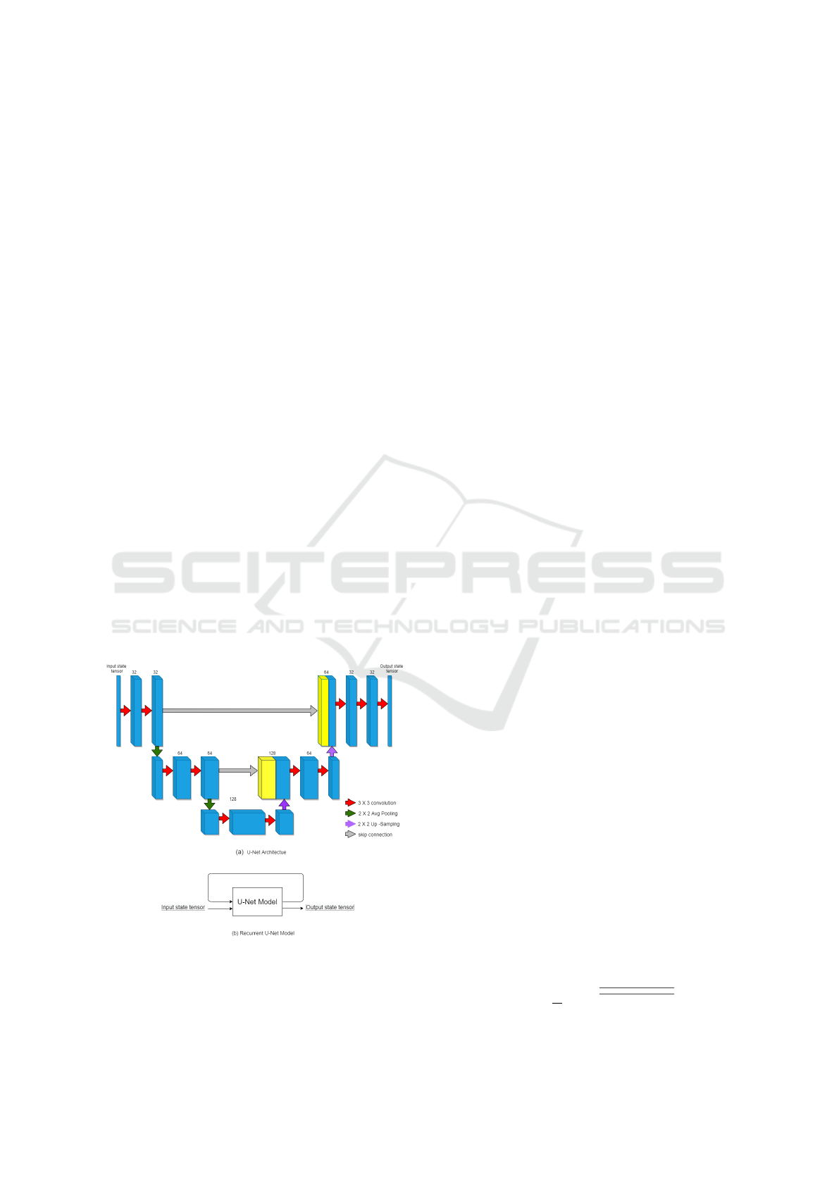
In Figure 1(a), each blue rectangle represents the

atmospheric state. The red arrows indicate a 2D con-

volution operation with relu as the activation func-

tion. The green arrow represents the average pool-

ing operation with stride 2. It is known as a ”down-

sampling operation”. Each purple arrow represents

Figure 1: CNN Architecture for weather model as a se-

quence of operations on layers

an upsampling operation. Due to average pooling

and up-sampling operations, some useful information

might get lost. To overcome this problem, the tensor

state of each convolution operation at the encoding

phase is exactly copied back to the tensor state of its

corresponding upsampling operation in the decoding

phase, as indicated by the grey arrow in Figure 1(a).

In order to enforce the model towards learning to

predict longer-term weather, the output obtained from

the U-Net architecture is again given as input to the

same U-Net, and sequentially, it performs all the op-

erations as shown in Figure 1(b). All the layers and

their corresponding shapes and trainable parameters

are mentioned in Table 1.

8 RECTIFIED LINEAR UNIT

As mentioned earlier, each convolution operation is

followed by a modiﬁed Leaky Rectiﬁed Linear Unit

(ReLu). For each input x, the leaky relu function is

given as follows:











0.1x x ≤ 0

x 0 ≤ x ≤ 10

10 x ≥ 10,

(3)

The max value of threshold (10) was set empirically.

9 TRAINING

We have trained the U-Net model with two param-

eters. (1) Time Interval (∆t) (2) i/O time steps. ∆t

denotes temporal resolution and i/O time step denotes

number of i/O instances considered for training and

testing. Each weather model is trained for a maxi-

mum of 50 epochs to avoid overﬁtting. We have intro-

duced an early stopping criterion for the model, which

stops the training if validation loss does not increase

in the last ﬁve epochs. To optimise the mean square

error (MSE) loss during the training phase, we have

used the Adam optimizer (Kingma and Ba, 2017) a

variant of the stochastic gradient descent optimization

algorithm, with a default learning rate of 0.001.

10 MODEL EVALUATION

The Forecast error is evaluated using the loss func-

tion RMSE. It computes the root mean square error

between the ground truth forecast vector x(t) and pre-

dicted forecast vector y(t). The RMSE is calculated

as follows:

RMSE =

∑

n=1

(x(t) − y(t))

(4)

Data-Driven Weather Forecast Using Deep Convolution Neural Network

855

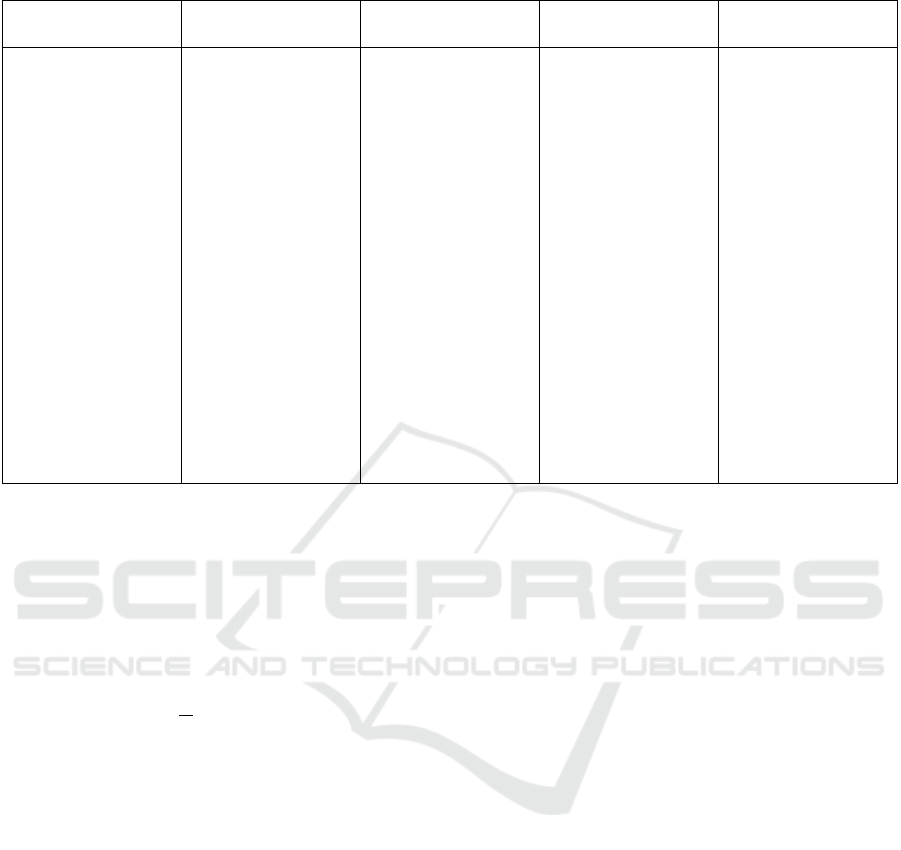
Table 1: CNN Architecture.

Layers Filters Filter size Output shape Trainable parame-

ters

CONV-2D 32 3 × 3 (48, 80, 32) 1184

CONV-2D 32 3 × 3 (48, 80, 32) 9248

Average Pooling-

– 2 x 2 (24, 40, 32)

CONV-2D 64 3 × 3 (24, 40, 64) 18496

CONV-2D 64 3 × 3 (24, 40, 64) 36928

Average Pooling-

– 2 × 2 (12, 20, 64)

CONV-2D 128 3 × 3 (12, 20, 128) 73856

CONV-2D 64 3 × 3 (12, 20, 64) 73792

Upsampling-2D – 2 × 2 (24, 40, 64)

Concatenate – – (24, 40, 128)

CONV-2D 64 3 × 3 (24, 40, 64) 73792

CONV-2D 32 3 × 3 (24, 40, 32) 18464

Upsampling-2D – 2 × 2 (48, 80, 32)

Concatenate – – (48, 80, 64)

CONV-2D 32 3 × 3 (48, 80, 32) 18464

CONV-2D 32 3 × 3 (48, 80, 32) 9248

CONV-2D 4 1 × 1 (48, 80, 4) 132

Here, the overbar indicates the average value over

all the spatial points on the grid. We have used

the Avg(Max) error and the Max(Max) error. The

Avg(Max) is calculated by ﬁnding the maximum

value over all the spatial locations and taking the aver-

age for each forecast step. The Avg(Max) error equa-

tion given as follows:

Avg(Max) =

∑

n=1

max

|x(t) − y(t)| (5)

max

is the maximum value over the spatial grid.

In equations (4) and (5), x(t) is the ground truth fore-

cast vector and y(t) is the predicted vector.

11 EXPERIMENTAL

EVALUATIONS

The dataset for each ﬁeld is divided into three differ-

ent sets. The training set consists of data from 1989 to

2005. The validation set consists of data from 2006 to

2016. The data from 2017 to 2018 was kept aside for

model testing. For proper use of data in a neural net-

work, the data must be internally consistent and in the

same format and type. We have used the data stan-

dardisation technique, in which every value is sub-

tracted from its mean and divided by its standard de-

viation, to ensure that the dataset becomes consistent.

Implementation details:

The weather model is implemented in Python using

the Keras API of the TensorFlow framework. The

processor is an Intel(R) Xeon(R) Gold 6139. The fol-

lowing paragraphs describe the analysis of results ob-

tained for different ﬁelds.

12 RESULTS

12.1 Importance of Solar Radiation

Data in Temperature Prediction

We conducted experiments to determine how solar ra-

diation affects temperature prediction. For that, we

trained two different U-net-based models and pre-

dicted results for the next six hours. The ﬁrst model

we trained with only temperature data, and for the

second model, we trained with both temperature and

solar radiation data. As shown in Figure 2, when we

trained the model without using solar data and pre-

dicted the results, the RMSE of the prediction was

ranging from 3.2 to 12.3, and the model with solar ra-

diation data was giving a RMSE in the range of 0.9 to

2.3. We can conclude from Figure 2 that solar radia-

tion plays a major role in the prediction of tempera-

ture data.

In meteorology, diurnal temperature variation is

the variation between a high and a low air tempera-

ture that occurs during the same day. In Figure 6.2, we

have plotted the mean and standard deviation graph of

the temperature w.r.t. each hour of the day. It can be

ICAART 2023 - 15th International Conference on Agents and Artiﬁcial Intelligence

856

Figure 2: Plot of Average spatial RMSE for the results without using solar data and with using solar data.

observed from the ﬁgure that solar radiation takes care

of the diurnal cycle of the day. Peak daily tempera-

tures occur in the afternoon, and similarly, minimum

daily temperatures occur after midnight.

12.2 Multi Field Prediction Using U-Net

Based Model

We have generated the results for multiple ﬁelds

based on two different parameters. i/o time steps

(number of input-output instances considered for

training and testing) and time resolution (temporal

resolution). For each time resolution, we have gen-

erated the results for all the deﬁned i/o time steps.

Given time instances, we have predicted all the input

ﬁelds mentioned in the dataset section for the next 6

instances. We predicted the results for ∆t = 1 hour, 2

hour and 3 hour and i/o time steps = 2, 3 and 4.

For example, if i/o time steps = 3 , ∆t= 3, and

the model is initialised at 1 January 00:00:00 UTC

then it will accept input as 1 January 21:00:00 UTC,

1 January 18:00:00 UTC and 1 January 15:00:00 and

will predict data of1 January 03:00:00 UTC, 1 Jan-

uary 06:00:00 UTC and 1 January 09:00:00 UTC.

Tables 2 and 3 show the accuracy of the model

based on two evaluation criteria: avg spatial RMSE

and Avg(Max) error for temperature and precipita-

tion, respectively. In each table, FH indicates the

forecast hour. I denotes i/o time steps. A repre-

sents actual avg spatial rmse and N(%) indicates nor-

malised avg spatial RMSE in percentage.

Figures 4 and 5 show the avg spatial RMSE and

Avg(Max) error as a function of forecast lead time up-

to next 6 time instances considering ∆t = 1 hour for

temperature and precipitation respectively. In each

ﬁgure, the left-side image indicates the plot of aver-

age spatial RMSE, and the right side image indicates

the plot of Avg(Max) error. The X-axis denotes the

forecast hour, and the Y-axis denotes the error rate for

each forecast hour. Forecast error plots for ∆t = 2 and

∆t = 3 are available in the GitHub repository linked in

the footnote

We also produced temperature and precipitation

heatmaps for each forecast hour using Deltat = 1 and

i/o time steps = 2, which are accessible at the refer-

ence listed in footnote

We have trained the ConvLSTM network pro-

posed in (Shi et al., 2015) using the dataset mentioned

in section 4. However, we have skipped a few prepro-

cessing steps while training the network. ConvLSTM

network is giving 1.13 avg. spatial RMSE for precip-

itation data, whereas U-Net is giving 0.41 avg. spatial

RMSE. The model’s output for other weather-related

ﬁelds is inaccurate. The models for different weather

ﬁelds are therefore not comparable.

13 DISCUSSION

In meteorology, diurnal temperature variation is the

variation between a high and a low air temperature

that occurs during the same day. It is observed dur-

ing experiments that the diurnal cycle of the day com-

pletely depends upon the solar radiations.

The weather data is the time series data. In U-Net

based model the solar radiation data takes care of the

time information of the day.

It is observed that in a U-Net-based model, adding

solar radiation data to the temperature ﬁeld during

training gives a much better result than training the

model alone with temperature data because the solar

data adds time information in the form of heat en-

ergy. The U-Net-based model performs better than

the NWP model. Global NWP models take around

3-6 hours to calculate physics-based equations. The

U-Net-based model takes around 4-5 minutes for pre-

www.github.com/Priya-Sharma07/Data-Driven-

Weather-Forecast-Using-Deep-Learning

Data-Driven Weather Forecast Using Deep Convolution Neural Network

857

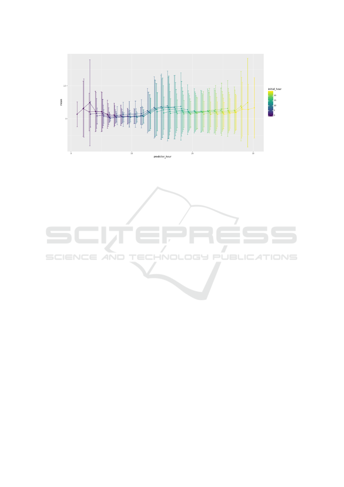
Figure 3: Plot of Average spatial RMSE for the results without using solar data and with using solar data.

diction once the model is trained. In DL-based mod-

els, it is needed to add the training data periodically.

The accuracy of the model can be increased by

increasing the training data.

14 CONCLUSION AND FUTURE

WORK

In this work, we have shown how deep learning meth-

ods can be used for multi-ﬁeld weather prediction

using available data. We have used the reanalysis

dataset for Madhya Pradesh state.

The diurnal cycle of the day completely depends

on the solar radiation. It adds the time information

to the i/p data in the form of heat energy. Peak daily

temperatures occur in the afternoon, and similarly, the

minimum daily temperature occurs substantially after

midnight. The U-Net model performs better than the

NWP model. It takes less time and resources to pre-

dict weather parameters. The NWP model uses one

forecasting system to predict a full array of weather

parameters. In contrast to this, DL based models can

be used to predict speciﬁc weather parameters.

In the future, we would like to improve the accu-

racy of the model by adding an attention mechanism

to the U-Net-based approach, as the mechanism al-

lows the model to focus and place more ”Attention”

on the relevant parts of the input sequence as needed.

We will also implement the preprocessing steps in the

ConvLSTM network and try to adapt the model for

other ﬁelds as well. so that we can make appropriate

comparisons among the models.

ACKNOWLEDGEMENTS

We are grateful to India Meteorological Department,

India and Indian Institute of Information Technology

Vadodara for providing the necessary support during

the work carried out.

REFERENCES

Bauer, P., Thorpe, A., and Brunet, G. (2015). The quiet

revolution of numerical weather prediction. Nature,

525:47–55.

Jakaria, A. H. M., Hossain, M. M., and Rahman, M. A.

(2020). Smart weather forecasting using machine

learning:a case study in tennessee.

Kingma, D. P. and Ba, J. (2017). Adam: A method for

stochastic optimization.

Shi, X., Chen, Z., Wang, H., Yeung, D.-Y., kin Wong, W.,

and chun Woo, W. (2015). Convolutional lstm net-

work: A machine learning approach for precipitation

nowcasting.

Sønderby, C. K., Espeholt, L., Heek, J., Dehghani, M.,

Oliver, A., Salimans, T., Hickey, J., Agrawal, S., and

Kalchbrenner, N. (2020). Metnet: A neural weather

model for precipitation forecasting. Submission to

journal.

Trebing, K., Stanczyk, T., and Mehrkanoon, S. (2021).

Smaat-unet: Precipitation nowcasting using a small

attention-unet architecture.

Weyn, J. A., Durran, D. R., and Caruana, R. (2020).

Improving data-driven global weather prediction us-

ing deep convolutional neural networks on a cubed

sphere. Journal of Advances in Modeling Earth Sys-

tems, 12(9).

Yamashita, R., Nishio, M., Do, R., and Togashi, K. (2018).

Convolutional neural networks: an overview and ap-

plication in radiology. Insights into Imaging, 9.

ICAART 2023 - 15th International Conference on Agents and Artiﬁcial Intelligence

858

APENDIX

Table 2: Temperature Error for ∆t = 1, ∆t = 2, ∆t = 3.

∆t = 1

I FH=1 FH=2 FH=3 FH=4 FH=5 FH=6

A N(%) A N(%) A N(%) A N(%) A N(%) A N(%)

Avg Spatial

RMSE

2 0.98 1.8 1.39 2.6 1.38 2.6 1.73 3.3 1.74 3.3 2.03 3.8

3 1.01 1.9 1.33 2.5 1.71 3.2 1.57 3.0 1.76 3.3 2.01 3.8

4 1.08 2.0 1.37 2.6 1.68 3.2 1.9 3.6 1.59 3.0 1.74 3.3

Avg Max

Error

2 0.16 0.41 0.55 0.76 0.81 1.01

3 0.18 0.44 0.72 0.7 0.83 1.01

4 0.21 0.46 0.7 0.84 0.72 0.81

∆t = 2

I FH=2 FH=4 FH=6 FH=8 FH=10 FH=12

A N(%) A N(%) A N(%) A N(%) A N(%) A N(%)

Avg Spatial

RMSE

2 1.65 3.1 3.36 6.3 3.26 6.1 5.11 9.6 4.1 7.7 5.06 9.6

3 1.84 3.5 3.96 7.5 6.1 11.5 4.54 8.6 6.06 11.4 7.85 14.8

4 2.05 1.9 4.54 2.5 6.64 3.2 8.08 3.0 5.3 3.3 6.48 3.8

Avg Max

Error

2 0.5875 1.7683 1.8038 2.9025 2.44 3.0606

3 0.787 2.2353 4.0267 2.8723 4.0257 5.663

4 0.9493 2.6392 4.3846 5.6745 3.5761 4.3093

∆t = 3

I FH=3 FH=6 FH=9 FH=12 FH=15 FH=18

A N(%) A N(%) A N(%) A N(%) A N(%) A N(%)

Avg Spatial

RMSE

2 3.88 7.3 7.49 14.1 6.01 11.3 9.16 17.3 7.11 13.4 9.7 18.3

3 3.91 7.4 7.5 14.2 9.52 18.0 8.02 15.1 9.57 18.1 10.19 19.2

4 4.97 9.4 8.67 16.4 10.13 19.1 9.16 17.3 9.11 17.2 11.81 22.3

Avg Max

Error

2 2.163 5.385 4.242 7.058 5.341 7.571

3 2.176 5.361 7.171 5.755 7.361 8.044

4 3.017 6.28 7.662 7.057 7.126 9.464

Figure 4: Average Spatial RMSE and Avg(Max) Error for Temperature Considering ∆t = 1.

Data-Driven Weather Forecast Using Deep Convolution Neural Network

859

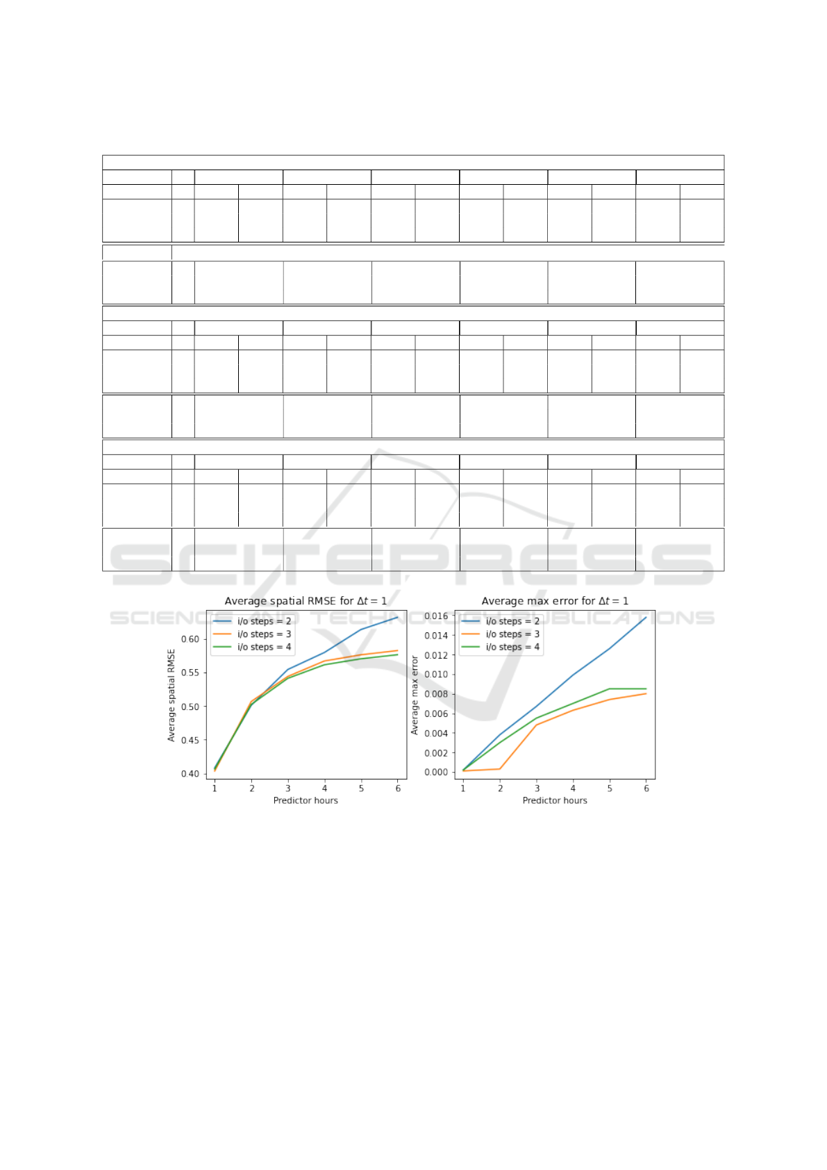
Table 3: Precipitation Error for ∆t = 1, ∆t = 2, ∆t = 3.

∆t = 1

I FH=1 FH=2 FH=3 FH=4 FH=5 FH=6

A N(%) A N(%) A N(%) A N(%) A N(%) A N(%)

Avg Spatial

RMSE

2 0.41 0.5 0.5 0.6 0.55 0.6 0.58 0.7 0.61 0.7 0.63 0.7

3 0.4 0.5 0.51 0.6 0.54 0.6 0.57 0.6 0.58 0.7 0.58 0.7

4 0.41 0.5 0.5 0.6 0.54 0.6 0.56 0.6 0.57 0.6 0.58 0.7

Avg Max

Error

2 0.0002 0.0038 0.0067 0.0099 0.0126 0.0158

3 0.0001 0.0003 0.0048 0.0063 0.0074 0.008

4 0.0002 0.003 0.0055 0.007 0.0085 0.0085

∆t = 2

I FH=2 FH=4 FH=6 FH=8 FH=10 FH=12

A N(%) A N(%) A N(%) A N(%) A N(%) A N(%)

Avg Spatial

RMSE

2 0.49 0.6 0.54 0.6 0.57 0.7 0.58 0.7 0.6 0.7 0.6 0.7

3 0.47 0.5 0.54 0.6 0.58 0.7 0.59 0.7 0.6 0.7 0.6 0.7

4 0.49 0.5 0.55 0.6 0.58 0.6 0.6 0.6 1.28 0.7 0.75 0.7

Avg Max

Error

2 0.0016 0.0057 0.0088 0.01 0.0117 0.0148

3 0.0014 0.0053 0.0088 0.0086 0.0104 0.012

4 0.0026 0.0084 0.0134 0.0194 0.1605 0.0494

∆t = 3

I FH=3 FH=6 FH=9 FH=12 FH=15 FH=18

A N(%) A N(%) A N(%) A N(%) A N(%) A N(%)

Avg Spatial

RMSE

2 0.53 0.6 0.59 0.7 0.61 0.7 0.62 0.7 0.62 0.7 0.63 0.7

3 0.53 0.6 0.59 0.7 0.61 0.7 0.62 0.7 0.63 0.7 0.63 0.7

4 0.55 0.6 0.62 0.7 0.63 0.7 0.64 0.7 0.75 0.8 0.73 0.8

Avg Max

Error

2 0.005 0.014 0.014 0.019 0.017 0.02

3 0.005 0.014 0.015 0.016 0.021 0.016

4 0.006 0.021 0.02 0.017 0.042 0.057

Figure 5: Average Spatial RMSE and Avg(Max) Error For Precipitation Considering ∆t = 1.

ICAART 2023 - 15th International Conference on Agents and Artiﬁcial Intelligence

860