Optimization of Circular Conveyor Belt Systems with Multi-Commodity

Network Flows

Antonin Novak

, Matous Pikous

1,2

and Zdenek Hanzalek

Czech Institute of Informatics, Robotics and Cybernetics, Czech Technical University in Prague, Czech Republic

Faculty of Electrical Engineering, Czech Technical University in Prague, Czech Republic

Keywords:

Circular Conveyor Belts, Manufacturing, Multi-Commodity Network Flow, Mixed-Integer Linear

Programming.

Abstract:

Modern industrial production with alternative process plans and the use of complex machine equipment in-

creases requirements for its intralogistics operations in terms of efﬁciency, resilience, and ﬂexibility. One of

the most common solutions for transporting workpieces between the manufacturing stations is a system of

conveyor belts where each conveyor rotates in a ﬁxed direction at a constant speed. The movement of the in-

dividual workpieces can be controlled only indirectly via a set of gates connecting different carousels. In this

paper, we aim to increase the ﬂexibility of conveyor belt systems by carefully scheduling the gates to route the

workpieces efﬁciently along the production line according to their process plans. The key component of our

solution is the discretization of both the time and positions on the belts to represent the system by a directed

graph with circular components. To ﬁnd the routing of workpieces that minimizes the total ﬂow time, we have

reduced the problem to the integer multi-commodity ﬂow on the time-expanded network with an extension for

the vertex precedences. Despite the simplicity of the formulation, the results suggest that off-the-shelf solvers

can ﬁnd optimized routing for instances with tens of workpieces and more than hundreds of belt positions

within a few minutes.

1 INTRODUCTION

One of the core concepts in Industry 4.0 is a highly

ﬂexible and customized production. To keep up

with the rising demand for many variants of prod-

ucts, deployment of more complex machine equip-

ment such as reconﬁgurable manufacturing systems

(RMS) (Fatemi-Anaraki et al., 2022) and intelligent

internal logistics systems are required. Due to the

fact that products are highly customized, they no

longer follow the identical production process plan,

but rather different product variants need to visit dif-

ferent manufacturing stations. Therefore, the stations

are interconnected with a transport system that moves

workpieces over the shop ﬂoor.

The transport and routing can be realized with,

e.g., autonomous ground vehicles (AGV) (Qiu et al.,

2002) or monorail systems such as Montrac, which

use an individual transport platform to handle the

movement of each workpiece separately. Although

these systems are very ﬂexible, they share certain dis-

advantages, such as low throughput and high cost.

Another option is conveyor belt systems, such as

the one shown in Figure 1. Here the difference is

that the system consists of several individual circular

Figure 1: Conveyor belt in Testbed for Industry 4.0 at

CIIRC CTU.

conveyor belts interconnected with controllable gates.

Each individual belt has its independent asynchronous

electric motor that rotates the belt at a constant speed.

Therefore, all pieces sharing the same belt are moved

simultaneously in the direction deﬁned by the drive

movement. If a piece needs to be transported to a ma-

chine located at a different belt, the piece needs to

stay on the belt before reaching a speciﬁc gate which

is switched at the right moment to transfer the piece

to a different belt. The advantage of conveyor belt

systems is that they are cheaper to operate and of-

Novak, A., Pikous, M. and Hanzalek, Z.

Optimization of Circular Conveyor Belt Systems with Multi-Commodity Network Flows.

DOI: 10.5220/0011784800003396

In Proceedings of the 12th International Conference on Operations Research and Enterprise Systems (ICORES 2023), pages 203-210

ISBN: 978-989-758-627-9; ISSN: 2184-4372

 2023 by SCITEPRESS – Science and Technology Publications, Lda. Under CC license (CC BY-NC-ND 4.0)

203

1 2

1412

1516

2122

25 26

313233343536

37 30

B A

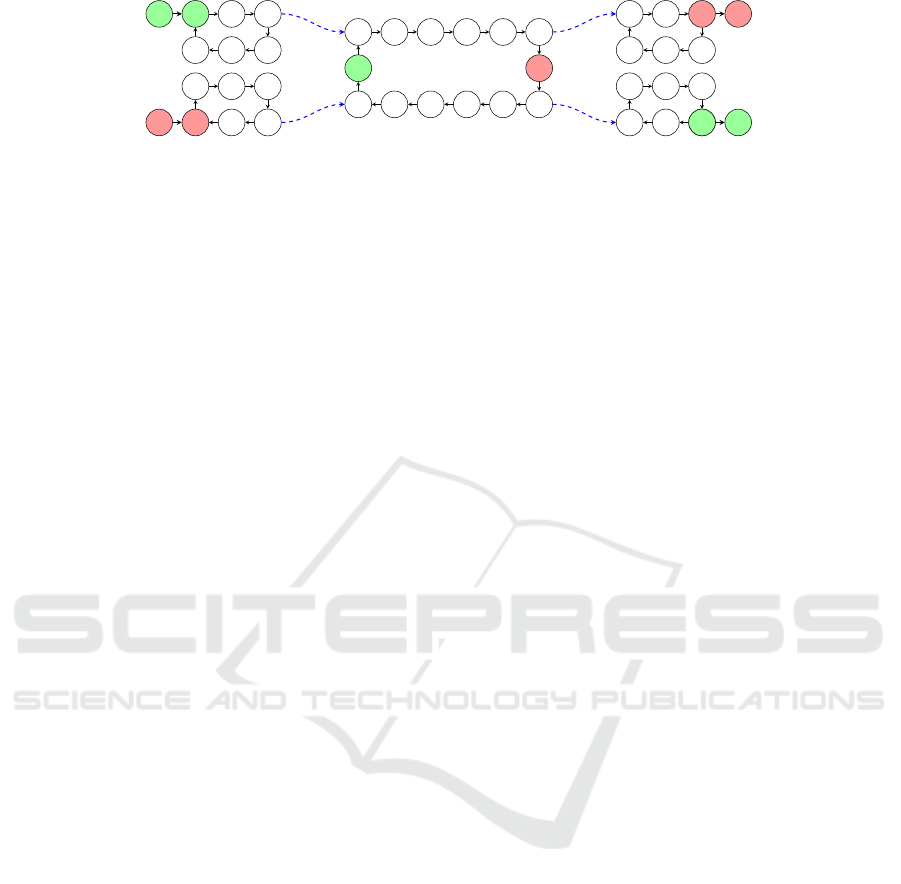
Figure 2: System model with ﬁve clockwise-rotating carousels, four gates, and two workpieces, each with three stations to

visit.

fer higher capacity. However, they are less ﬂexible as

the individual piece movement is controlled only in-

directly by the gate switches. Moreover, the individ-

ual conveyor belts are shared resources in the system;

thus, one needs to carefully schedule access to them,

e.g., to prevent collisions of pieces when switching

the belts.

In this work, we aim to improve the ﬂexibility of

conveyor belt systems by careful scheduling of opera-

tions. The inspiration was taken from the Testbed for

Industry 4.0 located at the Czech Technical University

in Prague (Nov

ak and Vysko

cil, 2022), where a set

of machine tools and robots is interconnected with a

system of conveyor belts with controllable gates (see

Figure 1). Our main idea is to discretize time and

positions on the belts and model the system with a

graph consisting of circular components, as depicted

in Figure 2. Then, we employ an extended inte-

ger multi-commodity ﬂow problem formulation for a

time-expanded system graph to ﬁnd optimal routing

for the set of workpieces while visiting all requested

stations without collisions. The proposed formalism

easily allows for the minimization of different crite-

ria expressed as a function of the completion times of

pieces, such as the makespan or the total ﬂow time.

The experiments demonstrate that even though the re-

sulting optimization models are quite large, the un-

derlying network ﬂow structure of the problem allows

mixed-integer linear programming solvers to retain

impressive scaling capability. Speciﬁcally, the main

contributions of this paper are:

(i) proposing a discretized model of a circular con-

veyor belt system and the optimization problem

of workpiece routing with a sequence of stations

to visit,

(ii) a formulation of the problem via integer multi-

commodity ﬂow problem on a time-expanded

network with the extension for vertex prece-

dences,

(iii) the experimental evaluation of the proposed

mixed-integer linear programming model.

2 RELATED WORK

One of the most frequently appearing applications

of the conveyor belt systems can be seen in vari-

ous package sorting tasks, e.g., in fulﬁllment centers.

For example, in (Chen et al., 2021), a simulation-

optimization approach is proposed to improve the

processing capacity of a circular conveyor belt in a

parcel sorting system by designing skip connections

to improve the processing capacity. However, the

conveyor belt layout is often ﬁxed and is not subject

to optimization. In these cases, the scheduling of op-

erations can be applied to improve the utilization of

the system. For example, (Bock and Bruhn, 2021)

study the problem of mould injection for product cast-

ing with a circular conveyor belt. In their problem,

they also consider a circular conveyor belt with sev-

eral robotic stations which perform activities on the

workpieces traveling on the belt.

From the perspective of the underlying optimiza-

tion problem, our problem is closely related to the

multi-agent path-ﬁnding problem (MAPF) (Bart

et al., 2018). The MAPF is among the classical prob-

lems in the literature, being studied under many dif-

ferent settings (Stern et al., 2019). The classical ver-

sion of MAPF assumes that a set of agents need to ﬁnd

paths on an undirected graph from their sources to the

destinations such that they avoid conﬂicts at all ver-

tices. However, such a setting does not apply to our

problem since our agents (i.e., workpieces) operate on

a directed graph, they cannot wait at an arbitrary ver-

tex to avoid collisions, they need to visit multiple lo-

cations in a speciﬁc order, and they do disappear at

target (Stern et al., 2019).

Another related, but more general, optimization

problem is the resource-constrained shortest path

problem (RCSPP) (Pugliese and Guerriero, 2013).

RCSPP at its most general setting speciﬁes a set of

resources and so-called resource extension functions

(REFs) which adjust the values of resources along the

found s-t path in the given graph. However, the ma-

jority of the existing efﬁcient algorithms for RCSPP

consider speciﬁc subsets of the problem, such as non-

decreasing REFs, rather than the general case. What

ICORES 2023 - 12th International Conference on Operations Research and Enterprise Systems

204

1 2

time = 0

1 2

time = 1

1 2

time = 2

1 2

time = 3

(a) Infeasible solution: conﬂict in vertex 12 at time 3.

1 2

(b) Feasible solution: conﬂict is avoided by postponing the transfer of B to the other belt by one rotation.

1 2

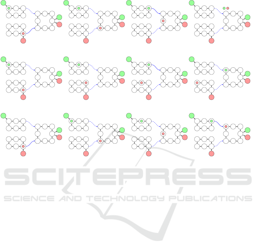
Figure 3: Examples of different solutions.

is more, when k workpieces are present, we need to

ﬁnd k vertex-disjoint paths, which further complicates

the modeling as an RCSPP.

Although the studied problem displays common

characteristics with the existing problems, such as

MAPF or RCSPP, we are not aware of any existing

problem or an algorithm that would efﬁciently encap-

sulate the problem addressed in this work.

3 SYSTEM MODEL

3.1 Model Description

In this section, we describe the assumptions behind

the used system model, and we formally deﬁne the

problem statement. Similarly as (Bock and Bruhn,

2021), we assume that positions on the belt and time

instants are discretized, meaning that each belt can

transport at any moment only a ﬁnite number of

pieces. Indeed, this is a reasonable assumption be-

cause the pieces on the belt are spaced out by sufﬁ-

cient margins to avoid problems. Thus, we assume

that each belt has a ﬁxed sense of rotation with the

speed of one position per time unit.

A conveyor belt system consists of several in-

dependent carousels interconnected by controllable

gates that can, at the speciﬁed moment, transfer a

workpiece from one belt to another. The workpiece

appears at its inbound location at its release time and

is ofﬂoaded to the belt at the time deﬁned by the

schedule. After the workpiece is ofﬂoaded to the

belt, it needs to visit a sequence of the required po-

sitions and is removed from the system as soon as

it reaches its outbound location. For the speciﬁc ex-

ample, see Figure 2. The displayed graph represents

the formalization of a system with two workpieces

and ﬁve carousels interconnected by four gates (de-

picted in blue). The workpiece A has to visit stations

0 −→ 37 −→ 21 while workpiece B visits 11 −→ 30 −→ 14.

The inbound and outbound locations for A are con-

nected to locations 0 and to 21, respectively. For B,

the inbound location is connected to 11, and the out-

bound to 14.

3.2 Problem Statement

The input to the problem consists of a directed graph

G = (V, E), which describes the system of conveyor

belts. It is assumed that G consists of a ﬁnite num-

ber of strongly connected components, where a com-

ponent is the cycle graph C

representing a carousel

with n positions. Next, we are given a set of gates

Optimization of Circular Conveyor Belt Systems with Multi-Commodity Network Flows

205

S ⊂ E, which represents controllable gates in the sys-

tem transporting workpieces between carousels.

The workload is represented by a set of k work-

pieces M = {1, . . . , k}. Each workpiece m ∈ M is

associated with the release time r

(m)

∈ N

, denoting

its earliest possible time when the workpiece can be

loaded on the belt. Before the workpiece is loaded

on the belt, it stays at its inbound location I

(m)

∈ V .

Furthermore, the workpiece m ∈ M speciﬁes the se-

quence of vertices (stations) π

(m)



(m)

, . . . , π

(m)



(m)

∈ V which have to be visited by m. After posi-

tion π

(m)

is reached by m, it is moved to its outbound

location O

(m)

∈ V and is effectively removed from the

system since it no longer occupies any belt position.

The solution to the problem is represented by

a schedule y

(m)

∈ V , which for each workpiece m

speciﬁes the position it occupies at time t. Further-

more, it deﬁnes for each gate (u, v) ∈ S a binary value

(u, v) ∈ {0, 1} which is set to 1 if and only if the gate

(u, v) is activated at time t.

We say that the schedule is feasible if workpieces

satisfy their release times and for any m

, m

∈ M,

6= m

: ∀t : y

)

6= y

)

, i.e., at any moment, no

two workpieces occupy the same position. Further-

more, a workpiece m which at time t occupies y

(m)

subsequently occupies its neighboring position of y

(m)

at time t +1. The neighboring position of vertex v ∈ V

at time t is either u ∈ V such that (v, u) ∈ E (i.e., u is

the successor position of the v on the same carousel)

or w ∈ V if (v, w) ∈ S and z

(v, w) = 1, i.e., the work-

piece is transported to a different carousel with (v, w)

gate. The objective is to minimize the total ﬂow time,

i.e., the sum of differences between the time reaching

the outbound location and the release time over every

workpiece.

3.3 Example

To demonstrate the deﬁned quantities and constraints

of the problem, please see an example in Figure 3.

There, we depict three different solutions for the prob-

lem with two workpieces A and B. We assume that the

release times of both workpieces are equal to zero,

i.e., r

(A)

= r

(B)

= 0 and the sequences of stations to

visit are π

(A)

= (0, 15) and π

(B)

= (9, 15).

In Figure 3a, both workpieces are loaded to the

carousel at time t = 0, thus y

(A)

= 0 and y

(B)

= 9. At

the time t = 1, workpieces are moved to their neigh-

boring location. In this solution, the gate (9, 18) was

activated at time t = 0, i.e., z

(9, 18) = 1. In subse-

quent time instant, both workpieces are again moved

to their neighboring positions; therefore, y

(A)

= 1 and

(B)

= 18. After one additional move, the gate (2,12)

is activated at time 2 (i.e., z

(2, 12) = 1), thus, we

have y

(A)

= 12. However, this violates the feasibility

condition since y

(B)

= 12 as well, and the solution (a)

is infeasible.

A different solution is shown in Figure 3b. In this

case, the gate (9, 18) is not activated at time t = 0.

Therefore, the workpiece B is forced to perform one

additional rotation with its initial carousel before it is

(eventually) transferred. Thus, the conﬂict at position

12 is avoided at the expense of increased ﬂow time of

B by 6 time units.

Finally, the third solution is displayed in Fig-

ure 3c. Here, the workpiece B is unloaded onto the

carousel immediately at time t = 0, whereas work-

piece A waits at its inbound location until time t = 1.

Since A is released 1 time unit later than in solution

(a), it also avoids the conﬂict at position 12, but the

total ﬂow time is smaller than in solution (b).

The above examples show some important con-

siderations to be made when solving the problem—

both the timings of the gates as well the times when

the workpieces are loaded to the carousels affect the

quality of the solution. Thus, they need to be consid-

ered simultaneously, which represents an interesting

optimization problem.

4 TIME-EXPANDED INTEGER

MULTI-COMMODITY FLOW

First, we explain the concept of a time-expanded net-

work for the conveyor belt scheduling problem. Then,

we give a mixed-integer linear programming (MILP)

formulation of the problem, which resembles an ordi-

nary integer multi-commodity network ﬂow problem

with one additional constraint.

4.1 Time-Expanded Network

The main difﬁculty of using network ﬂow formalism

for problems with time-related constraints (e.g., re-

lease times and vertex ordering) is that a ﬂow in the

network does not capture the notion of time. One of

the possible options how to accommodate these con-

straints is the so-called time expansion of the network,

which is used, e.g., for dynamic network ﬂow prob-

lems (Ahuja et al., 1988).

A B

Figure 4: An example of a system G.

ICORES 2023 - 12th International Conference on Operations Research and Enterprise Systems

206

The core idea of the time expansion is to con-

struct copies of the original graph, where each copy

represents the network at a speciﬁc time instant. The

copies of the original network are connected in a way

that represents possible state transitions between the

past and future time instants. In our case, the time-

expanded network G = (V , E) of the conveyor belt

system G = (V, E) is constructed as follows. First,

the value of time horizon H ∈ N needs to be chosen

such that all workpieces m ∈ M can visit their stations

(m)

and reach the outbound location O

(m)

within H

time steps.

Next, for each time instant within the horizon H,

one copy of the network, except for inbound and out-

bound locations, is created as a so-called layer. At

each layer, all edges that exist in the original graph

G, i.e., the representation of belt rotations and the po-

sitions of the gates, are removed. Instead, an edge

between vertex v in layer t and vertex u in layer t + 1

is introduced, if and only if u is possible neighboring

vertex of v at time t in G, i.e., either u is a succes-

sor position on the conveyor or (v, u ) ∈ S is a gate.

Finally, for each inbound I

(m)

and outbound location

(m)

a corresponding vertex is added to V .

Note that the edges E in time-expanded network

G can be uniquely associated with a speciﬁc time in-

stant. Indeed, each outgoing edge from any vertex

i ∈ V can be assigned to a time instant t correspond-

ing to in which layer t the vertex i is contained. Ad-

ditionally, an edge leaving inbound location I

(m)

can

be associated with time instant t − 1 if it enters a ver-

tex v in layer t. In this way, every edge e ∈ E in a

time-expanded network can be described with a triplet

(t, i, j) ∈ E. To model the release time constraint for a

workpiece m ∈ M, we introduce a single vertex repre-

senting inbound location I

(m)

and connect it with the

position π

(m)

in every layer t ≥ r

(m)

. Similarly, π

(m)

location at every layer t ≥ r

(m)

is connected to a single

outbound location O

(m)

To demonstrate the structure of the time-expanded

network, let us consider a system described by the

graph G in Figure 4 with the parameters of work-

pieces given in Table 1. The resulting time-expanded

network G with horizon H = 4 (i.e., in total ﬁve lay-

ers including the time instant t = 0) can be seen in

Figure 5.

Table 1: Example parameters of workpieces.

workpiece m stations π

(m)

release time r

(m)

A 3 −→ 7 1

B 5 −→ 6 2

4.2 Integer Multi-Commodity Flows

with Vertex Precedences

Having the time expansion of the network, the move-

ments of the workpieces can be modeled as ﬂows

transported from their inbound to the outbound lo-

cations. To consider the individual identities of the

ﬂows, they need to be modeled as different commodi-

ties to prevent that, e.g., the workpiece A would reach

outbound location O

(B)

instead of O

(A)

. The integer

multi-commodity ﬂow problem speciﬁes the set of k

commodities to be transported over a directed net-

work G and a k-dimensional balance vector b(v) for

each vertex v ∈ G. In our case, we set b

(m)

) = 1,

(m)

) = −1, ∀m ∈ M and for all other vertices v

we set b

(m)

(v) = 0, ∀m ∈ M. The objective function is

the sum of costs for all edges times the amount of ﬂow

transported over the edge. The cost of all edges e ∈ E

is equal to zero except the edges (v, O

(m)

) that have

cost t − r

(m)

if v is a vertex in layer t. In this way, we

model minimizing the total ﬂow time of workpieces

m ∈ M.

As a next constraint, we need to ensure that, at

most, one unit of a ﬂow can enter any vertex to avoid

situations such as the one depicted in Figure 3a at

time t = 3. This constraint can be easily accommo-

dated into multi-commodity network ﬂow formalism

by the vertex expansion (Ahuja et al., 1988). Further-

more, the solution needs to enforce that if for some

workpiece m ∈ M and its station sequence π

(m)



(m)

, . . . , π

(m)

, . . . , π

(m)

, . . . , π

(m)



the π

(m)

is visited

at time t

, and π

(m)

is visited at time t

, then t

< t

However, from the perspective of a solution, it is im-

portant to distinguish whether the workpiece m ∈ M

visits the station π

(m)

in a sense as it is given by the

problem statement (i.e., operating on the workpiece),

or whether it transits through the position to reach a

different destination. Although this seems obvious, it

introduces surprising difﬁculties when modeling the

problem with an ordinary multi-commodity network

ﬂow. Therefore, we introduce an extension of unit-

capacity integer multi-commodity ﬂows that we call

vertex precedences. A vertex precedence for com-

modity m ∈ M is given in the form of i −→ j, where

i, j ∈ V are vertices in the original graph G. The con-

straint requires that the resulting ﬂow of the commod-

ity m in the time-expanded network G transits through

the vertex i in layer t

and the vertex j in layer t

, such

that t

< t

An inconvenient property of this extension is that

it disqualiﬁes the use of the existing algorithms for the

multi-commodity network ﬂow problem. However,

we note that the original integer multi-commodity

Optimization of Circular Conveyor Belt Systems with Multi-Commodity Network Flows

207

A B

Figure 5: Example of a time-expanded network G.

network ﬂow problem is NP-hard already for two

commodities even when restricted to networks with

unit capacities (Garey and Johnson, 1979). Therefore,

even if there would be an efﬁcient way of accommo-

dating vertex precedences into the ordinary integer

multi-commodity ﬂow problem, a substantial com-

plexity is already introduced by the formalism itself.

Nevertheless, the practical experience with mixed-

integer linear programming (MILP) formulations of

the integer multi-commodity ﬂow problem indicates

that even large instances can be solved in a reason-

able time.

4.3 MILP Model

Let T = {0, 1, . . . , H − 1} be a set of all time instants

within the horizon H. The main decision variable is

(m)

(i, j) ∈ {0, 1} with the meaning whether the com-

modity m is transported along the edge (t, i, j) ∈ E in

time-expanded network G. Furthermore, we use a bi-

nary indicator x

(m)

t,i

, which enforces that the commod-

ity m leaves vertex i at layer t. This variable is used

to enforce the vertex precedence constraints. With the

above, we state the full model as:

min

∑

t∈T

∑

m∈M

∑

i∈V

(t − r

(m)

) · f

(m)

(i, O

(m)

) (4.1)

subject to

∑

(t,v, j)∈E

(m)

(v, j) −

∑

(t−1,i,v)∈E

(m)

t−1

(i, v) = b

(m)

(v)

∀v ∈ V , ∀m ∈ M (4.2)

∑

m∈M

∑

(t,i,v)∈E

(m)

(i, v) ≤ 1 ∀v ∈ V (4.3)

∑

j∈V

(m)

(i, j) ≥ x

(m)

t,i

∀t ∈ T, ∀i ∈ π

(m)

(4.4)

∑

t∈T

(m)

t,i

= 1 ∀m ∈ M, ∀i ∈ π

(m)

(4.5)

∑

t∈T

(m)

t,i

·t + 1 ≤

∑

t∈T

(m)

t, j

·t ∀m ∈ M, ∀(i −→ j) ∈ π

(m)

(4.6)

(m)

(i, j) ∈ {0, 1} ∀m ∈ M, ∀(t, i, j) ∈ E (4.7)

(m)

t,i

∈ {0, 1} ∀m ∈ M, ∀t ∈ T, ∀i ∈ π

(m)

. (4.8)

The objective (4.1) represents the minimization of

the total ﬂow time. Flow conservation constraint is

expressed by (4.2). Since the value of b

(m)

(v) is set as

described in Section 4.2, the constraint (4.2) also en-

forces that workpiece m appears at inbound location

(m)

and eventually reaches its outbound O

(m)

. The

constraint (4.3) models vertex capacities to enforce

that, at most, one workpiece occupies a belt position

at any time.

Finally, the constraints (4.4)–(4.6) are used to

model vertex precedence constraints. If variable x

(m)

t,i

is set to 1, then we interpret it such that an operation

is performed on the workpiece m at time t. There-

fore, we require that such the operation i ∈ π

(m)

performed exactly once by constraint (4.5), and the

corresponding commodity must enter (and leave) the

speciﬁc vertex at the required time by constraint (4.4).

The correct ordering of vertices in π

(m)

is enforced

by (4.6). For any two consecutive elements of the

station sequence (i −→ j) ∈ π

(m)

the model computes

the times when the operations are performed by terms

∑

t∈T

(m)

t,i

·t and

∑

t∈T

(m)

t, j

·t. Then, it is enforced that

the time of the operation in the vertex i is smaller than

in j.

ICORES 2023 - 12th International Conference on Operations Research and Enterprise Systems

208

5 EXPERIMENTS

The performance of the proposed multi-commodity

ﬂow model has been assessed by the following set

of experiments. The key parameters that inﬂuence

the complexity of a problem instance are (i) the num-

ber of workpieces, (ii) the number of stations to visit,

(iii) the number of belts and their total length, and

(iv) the length of the time horizon. The speciﬁc range

of the values used for these parameters is described

in each experiment. The instances were generated

such that the resulting system of conveyor belts is a

strongly connected graph.

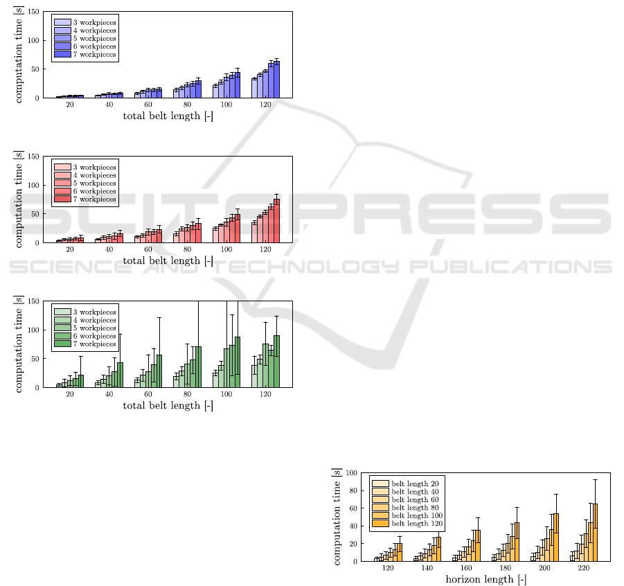
(a) Instances with two stations.

(b) Instances with three stations.

Figure 6: Effect of the number of required stations on com-

putational time.

The time expansion of the graph was performed in

Python 3. The resulting MILP formulation was solved

with the Gurobi 9.1.1 solver utilizing at most eight

threads of Intel Xeon E5-2690 CPU. The measured

CPU times reﬂect both the time spent by time expan-

sion as well as the computation time of the solver.

5.1 Effect of the Number of Stations

To assess how the computational time scales with re-

spect to the number of required stations, we have

performed the following set of experiments with the

varying numbers of stations required. In total, we

have generated 3360 instances with |M| ∈ {3, . . . , 7}

workpieces, total belt length was generated in interval

[20, 120] and the number of required stations by all

workpieces m ∈ M was |π

(m)

| ∈ {2, 3, 4}. The length

of time horizon H was set to 180.

The results are displayed in Figure 6. Each graph

displays mean computational times with standard de-

viations grouped by the total belt length and the num-

ber of workpieces M. As expected, the complexity of

an instance depends largely on the number of required

stations as it introduces additional variables (4.8) and

deteriorates the structure of the problem further from

the ordinary multi-commodity ﬂow. The main chal-

lenges for the model appear with instances with four

stations. There, we can see that the computational

times start to ﬂuctuate under the presence of outliers

represented by the occasional long running time of

the solver. The practical experience with the solver

behavior has revealed that the optimal solution is of-

ten attained soon after the root node is solved. How-

ever, this follows after quite a long preprocessing step,

which greatly reduces the size of the model. There-

fore, it seems that improvements in the optimization

model are possible.

5.2 Effect of the Horizon Length

The experiments in Section 5.1 were run with the

ﬁxed length of the time horizon H. To test its in-

ﬂuence on the computation time, we have ﬁxed the

number of stations to 3 and generated a total of 1120

instances varying in the total belt length that was

set to be contained within [20, 120]. This set of in-

stances was solved with time horizon lengths H ∈

{120, 140, . . . , 220}. The results are displayed in Fig-

ure 7.

Figure 7: Scaling with respect to the length of the hori-

zon H.

As suggested by our preliminary experiments, the

Optimization of Circular Conveyor Belt Systems with Multi-Commodity Network Flows

209

length of the time horizon has only a moderate effect

on the overall computation time.

6 CONCLUSION

We studied the problem of optimal routing for the set

of workpieces in a system of circular conveyor belts

where the movement of workpieces cannot be directly

affected, but they can be controlled indirectly via the

set of gates connecting different carousels. Our main

idea used in the solution is to discretize the time and

positions on the belts and to model the system with

a graph consisting of circular components. Then we

formulate it as an integer multi-commodity ﬂow prob-

lem for a time-expanded system graph with the vertex

precedence constraint.

For future work, we suggest considering the en-

ergy consumed by the system. At certain moments,

the belts might be switched to a power-saving mode,

e.g., by reducing the speed of the movement or shut-

ting down completely.

ACKNOWLEDGEMENTS

This work was supported by the EU and the Ministry

of Industry and Trade of the Czech Republic under the

Project OP PIK CZ.01.1.02/0.0/0.0/20 321/0024399.

REFERENCES

Ahuja, R. K., Magnanti, T. L., and Orlin, J. B. (1988). Net-

work ﬂows.

Bart

ak, R.,

Svancara, J., and Vlk, M. (2018). A scheduling-

based approach to multi-agent path ﬁnding with

weighted and capacitated arcs. In AAMAS’18, pages

748–756.

Bock, F. and Bruhn, H. (2021). Case study on scheduling

cyclic conveyor belts. Omega, 102:102339.

Chen, T.-L. et al. (2021). Solving the layout design problem

by simulation-optimization approach–a case study on

a sortation conveyor system. Simulation Modelling

Practice and Theory, 106:102192.

Fatemi-Anaraki, S. et al. (2022). Scheduling of multi-robot

job shop systems in dynamic environments: Mixed-

integer linear programming and constraint program-

ming approaches. Omega, page 102770.

Garey, M. R. and Johnson, D. S. (1979). Computers and

intractability.

Nov

ak, P. and Vysko

cil, J. (2022). Digitalized automation

engineering of Industry 4.0 production systems and

their tight cooperation with digital twins. Processes,

10(2).

Pugliese, L. D. P. and Guerriero, F. (2013). A survey of re-

source constrained shortest path problems: Exact so-

lution approaches. Networks, 62(3):183–200.

Qiu, L., Hsu, W.-J., Huang, S.-Y., and Wang, H. (2002).

Scheduling and routing algorithms for AGVs: a sur-

vey. International Journal of Production Research,

40(3):745–760.

Stern, R. et al. (2019). Multi-agent pathﬁnding: Deﬁnitions,

variants, and benchmarks. In SoCS’19.

ICORES 2023 - 12th International Conference on Operations Research and Enterprise Systems

210