Fast Skeletons of Handwritten Texts in Digital Images
Leonid Mestetskiy and Dimitry Koptelov
Lomonosov Moscow State University, Moscow, Russia
Keywords: Polygonal Figure, Internal Skeleton, Voronoi Diagram, Sweeping Algorithm.
Abstract: The article considers the problem of constructing a Voronoi Diagram (VD) of a polygonal figure - a
polygon with polygonal holes. A planar sweeping algorithm is proposed for constructing the VD of the
interior of a polygonal figure with 𝑛 vertices, which has complexity 𝑂(𝑛 𝑙𝑜𝑔 𝑛). Two factors provide a
reduction in the amount of calculations and an increase in robustness compared to known solutions. This is
the direct construction of only the inner part of the VD, as well as the use of the pairwise incidence property
of linear segments formed by the sides of a polygonal figure. The proposed algorithm has been implemented
and practically tested for polygonal figures of dimension 𝑛~10

in studies on the analysis and recognition
of handwriting. Computational experiments illustrate the robustness and efficiency of the proposed method.
1 INTRODUCTION
A polygonal figure (PF) is a closed area on a plane,
the boundary of which consists of non-intersecting
simple polygons, i.e. it is a polygon with polygonal
holes. The skeleton or median axis of such a figure
is the set of points of the centers of the maximum
circles contained within the figure. Skeletons are
used in shape recognition tasks, in particular, for
recognizing handwritten text from digital images.
The image of the text is approximated by polygonal
figures, and then a skeleton is built for this set of
figures (Fig. 1) (Mestetskiy, 2008).
(a)
(b)
Figure 1: (a) the binary bitmap, (b) polygonal figure and
its skeleton.
Figures and skeletons in practical problems of
the analysis of archival handwritten documents have
large number of vertices of the order of 10
5
(Fig. 2).
The skeleton of PF is a subgraph of the
generalized Voronoi diagram (VD) of the set of site-
points and site-segments created from the vertices
and sides of the figure. Algorithms for constructing
VD and image skeletons of handwritten documents
are subject to high requirements for robustness and
computational efficiency for application in large
archives of digitized manuscripts. Therefore, when
choosing algorithms for practical use, their real
speed and robustness are important.
The computational efficiency of algorithms for
constructing skeletons and VD has always been in
the spotlight. The algorithm (Lee, 1982) builds the
inner skeleton of a simple n-gon in 𝑂(𝑛 𝑙𝑜𝑔 𝑛) time.
Later, a solution appeared for multiply connected
polygonal regions (polygons with holes) with
complexity 𝑂(𝑛(𝑙𝑜𝑔 𝑛+ 𝑚)), where 𝑛 is the
number of polygon vertices and 𝑚 is the number of
holes (Srinivasan, 1987). However, this algorithm
for such images as in Fig.2, in which 𝑚=𝑂(𝑛),
spends 𝑂(𝑛

) time. Algorithms for constructing a
VD of a set of 𝑛 line segments (Fortune,1987),
having complexity 𝑂(𝑛 𝑙𝑜𝑔 𝑛), are a guideline for
developing more efficient solutions. Reducing the
PF to a finite set of linear segments can be done in
𝑂(𝑛) time. Later works develop the topic of
constructing theoretically efficient algorithms (Bae,
2015). However, the practical implementation of
these approaches faces the problem of algorithm
robustness.
The problem of robustness arises in solving
many problems of computational geometry. It
consists of the gap between theoretically correct
geometric algorithms and practical computer
Mestetskiy, L. and Koptelov, D.
Fast Skeletons of Handwritten Texts in Digital Images.
DOI: 10.5220/0011784600003417
In Proceedings of the 18th International Joint Conference on Computer Vision, Imaging and Computer Graphics Theory and Applications (VISIGRAPP 2023) - Volume 4: VISAPP, pages
435-443
ISBN: 978-989-758-634-7; ISSN: 2184-4321
Copyright
c
 2023 by SCITEPRESS – Science and Technology Publications, Lda. Under CC license (CC BY-NC-ND 4.0)
435

programs. This is mainly due to the fact that the
actual calculations contain numerical errors; these
errors sometimes cause inconsistencies in the
topology and thus lead to program crashes (Imai,
1996, Sugihara, 2000). When constructing a VD, the
source of such errors is the calculation of large
inscribed circles. The circle incident to the triple of
almost collinear sites has a very large radius, since
its center is the intersection point of the "almost
parallel" bisectors. To ensure the practical
robustness of algorithms, it is necessary to apply
various heuristic techniques focused on the features
of specific software solutions (Sugihara, 2000, Held,
2001, Menelaos, 2004). In this case, the theoretical
computational efficiency 𝑂(𝑛 𝑙𝑜𝑔 𝑛) is not
achieved.
Figure 2: Text approximation by polygonal figures: 244
connected components, 1258 polygons, 63556 vertices.
Skeleton: 95884 vertices, 96654 edges.
The solution proposed in this paper is based on
the special feature of the VD PF problem, which
allows one to reduce it to line segments VD in such
a way as to avoid fatal numerical errors. This feature
consists in the fact that it is necessary to find only
the inner part of the VD that lies inside the PF.
Therefore, if only inner parts are built, then such
errors can be avoided, since all the inner inscribed
circles of the figure do not exceed the size of the
figure itself. But this requires a special algorithmic
solution that will allow building only internal
circles.
This feature can also be used to improve the
computational efficiency of the algorithm. If the
outer part of the VD is not needed, then it becomes
possible to save on its calculations. Known
algorithms for constructing a VD PF do not take this
possibility into account. They build the VD of line
segments on the entire plane, and then select the
inner part in post-processing.
This article presents an algorithm for the direct
construction of a VD for the internal part of the PF,
based on the paradigm of sweepline. The proposed
solution includes new elements that make it possible
to build only the inner part of the VD PF. First, the
concept of oriented site-segments is introduced, for
which the inner side of the PF is defined. Secondly,
the data structure Sweepline Status, which is
traditionally present in sweepline algorithms, is built
as an ordered set of site zones. Such a structure is an
alternative to the traditionally used wave front or
coastline.
In addition, the algorithm takes into account the
specificity of the set of sites formed by the boundary
of a polygonal figure, namely, the incidence of each
point-site to two segment-sites and each segment-
site to two point-sites. This property helps to
perform a significant part of the operations in the
status in constant time. To do this, the status is
implemented as a combination of a balanced tree
and a doubly linked list.
2 INNER VORONOY DIAGRAM
The boundary of a polygonal figure consists of one
outer and several inner polygons. All of them are
described by sequences of their vertices in such a
way that the interior of the PF is to the left of the
boundary. Each boundary polygon is broken down
into subsets called sites. The vertices of the figure
define a set of sites-points, and the sides of the
figure define a set of sites-segments. Segment sites
have a direction in accordance with the direction of
the figure border, i.e. the interior of the shape lies to
the left of the segment site.
The locus of a site is the set of points in a figure
for which this site is the closest. This site is called
the generating site of the locus. And the closest site
for a point of a figure is determined by the position
of its closest point on the border of the figure. If the
closest point of the boundary coincides with the
vertex of the figure, then the site corresponding to
the vertex is the closest one. If the closest point is
the orthogonal projection of the figure's point onto
the segment site, then that site is the closest.
The boundary between a pair of loci consists of
points equidistant from their generating sites, and is
called the bisector of these sites. The set of bisectors
of all loci is called the internal Voronoi diagram. It
VISAPP 2023 - 18th International Conference on Computer Vision Theory and Applications
436

has the form of a geometric graph, the vertices of
which are the points of the figure, and the edges are
segments of straight lines and quadratic parabolas.
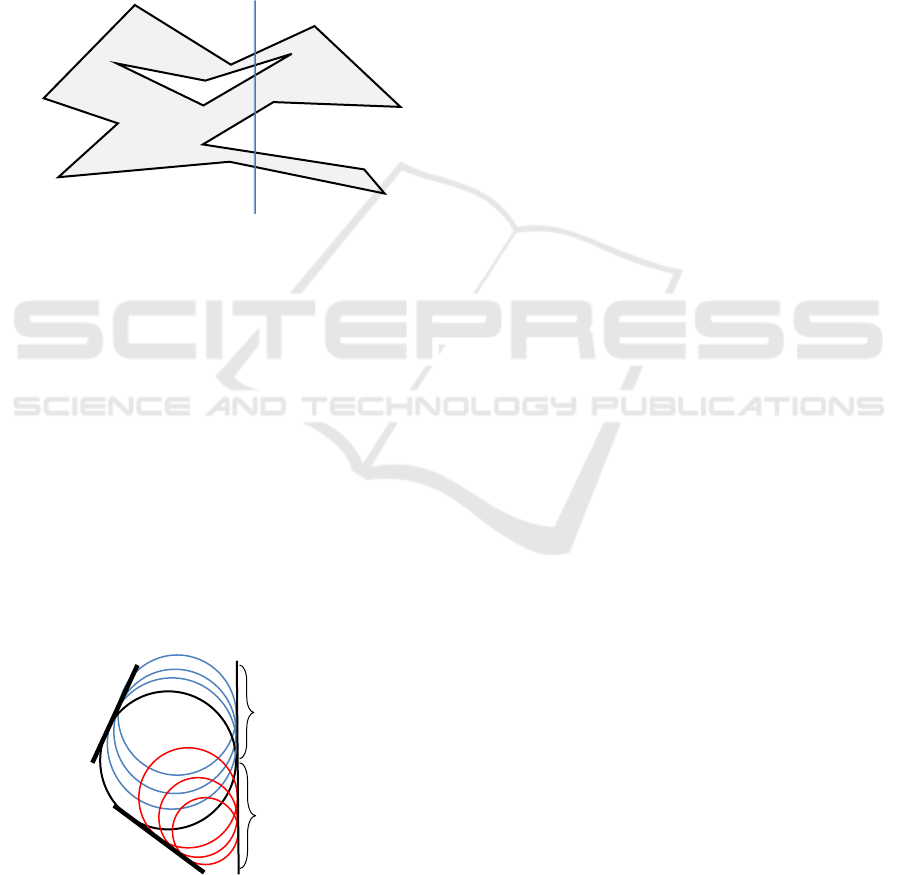
3 SECTIONS AND ZONES
The PF boundary can be represented as a finite set of
monotone branches. Each branch is a polyline, the
vertices of which are ordered lexicographically from
left to right (Fig. 3).
Figure 3: Monotone branches of the PF boundary: 1-12-
11-10-9, 7-6-5, 7-8-9, 3-4-5, 1-2, 3-2, 13-14-15, 13-16-15.
A sweeping line (SL) is a vertical line that
moves from left to right parallel to itself.
The branches break the sweeping line into
connected subsets, the so-called sections. The
sections inside the figures are called internal, outside
the figure - external (Fig. 3).
The internal sections, in turn, are divided into so-
called site zones, defined as follows. For each point
of the inner section, there is a maximum circle that
lies inside the figure in the left half-plane relative to
the sweeping line and touches it at this point. Since
the circle is maximal, it also touches the inside of the
figure's boundary at one or more points. Each touch
point belongs to a site. These sites and the circle are
called incident.
Figure 4: Zones of sites s
1
, s
2
. Circles of zone s
1
, s
2
are red
and blue. Common circle of two zones is black.
A site zone is a segment of a sweeping straight
line, all points of which have tangent circles incident
to this site. We will call this incident site the zone
generator (Fig. 4). For terminology convenience, the
external sections are also referred to as external
zones.
Thus, site zones and external zones cover the
entire SL. The order relation is defined on the set of
zones – from bottom to top. As the SL moves, this
set of zones changes: zones appear and disappear.
The zone at the moment of generation has a length
of 0, i.e. this is a point on the SL. As the straight line
moves to the right, it turns into a segment, the size of
the zone increases. Thereafter the size of the zone
decreases to zero, it degenerates into a point and
disappears.
The data structure that describes the ordered set
of zones on the SL is called the "status of the SL", as
in all sweepline algorithms (Preparata, 1985).
4 THE SWEEPING PROCESS
As the SL moves, all zones on it go through the
same life cycle: generation - resizing (growth and
contraction) - splitting (possible, but not mandatory)
- disappearance.
The dynamically changing neighborhood of
zones in the status of the SL completely determines
the structure of the VD. Therefore, the task is to
trace all status changes and identify all neighboring
pairs of zones in the changing status structure.
The connection between the neighborhood of
zones in the status and the edges and vertices of the
VD is determined by the following statements.
1. If two sites have a common tangent inscribed
circle, then there is such a position of the SL and
such a pair of adjacent zones in status, for which
these two sites are generators.
2. If two zones are adjacent in status, then the
generator sites of these zones have adjacent loci in
the VD, and the common boundary of these loci
describes an edge in the VD.
3. If three sites have a common tangent inscribed
circle, then there is such a position of the SL and
such a triple of adjacent zones in status, for which
these three sites are generators.
From Statements 1 and 2 it follows that each pair
of adjacent internal zones in the status defines a
Voronoi edge in the VD. This implies that if any two
zones become adjacent in the process of sweeping,
then the bisector of the sites-generators of these
zones is an edge of VD.
zone of s
2
site s
2
site s
1
zone of s
1
16
1
2
3
4
5
6
7
8
9
10
12
13
14
15
11
Fast Skeletons of Handwritten Texts in Digital Images
437

The adjacency of zones changes during
sweeping only at the points of events. A change in
the adjacency of zones occurs when new zones are
created and when existing ones disappear. The
generation of zones occurs when the SL passes
through the vertex of the PF. This position of the SL
is called a vertex event.
The new zone included in the status forms two
new adjacent pairs with the zones above and below
it. When a zone disappears and is excluded from its
status, two zones located above and below it form a
new pair of adjacent zones. These new pairs
automatically generate VD edges.
Statement 3 allows us to calculate the vertices of
the VD. As soon as any three zones become
neighbors in the status, we need to check if there is a
common inscribed tangent circle for the site
generators of these zones.
Thus, in order to find all vertices and edges of
the VD, it is necessary to track all pairs and triples
of adjacent zones in the status during sweeping.
5 INITIALIZATION OF ZONES
The general idea of the sweeping process is as
follows. The sweep line moves from left to right
discretely, occupying positions corresponding to the
moments of events. Each event leads to a change in
the status of the SL: the vertex event leads to the
appearance of new zones, and the circle event leads
to the exclusion of the zone from the status. At the
same time, the set of zones in the status retains order
in all changes.
Changes in the status lead to a change in the
neighborhood of zones on the SL. New neighboring
pairs and new triples of neighboring zones are
formed. Tracking status changes, we get all the
edges and vertices of the VD.
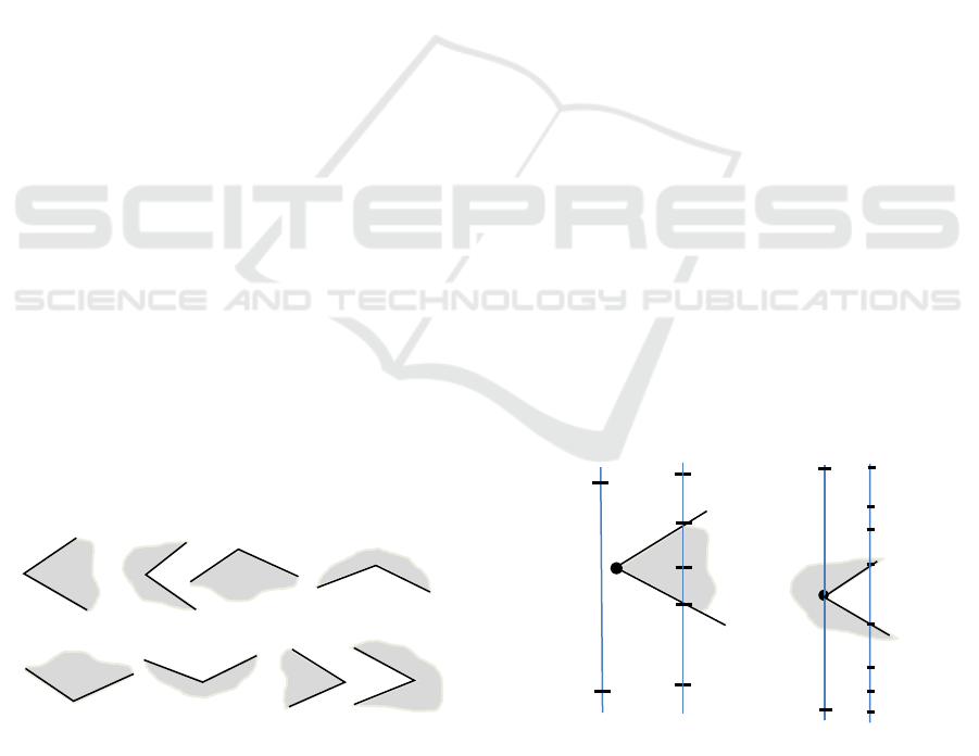
Figure 5: Types of vertices of a polygonal figure: left (a,
b), through (c, d, e, f), right (g, h), convex (a, c, e, g),
concave (b, d, f, h), lower (d, e) and upper (c, f). Interior
polygon is marked in grey.
Thus, in the process of sweeping, it is necessary
to make changes to the status for each event, identify
all newly formed neighboring pairs and triplets of
zones, and calculate the corresponding vertices and
edges of the VD.
Changes in status upon the occurrence of a
vertex event are determined by the vertex type.
There are 8 types of vertices in total (Fig.5).
Denote:
𝑣 is a vertex site formed by the vertex of the
polygon,
𝑠

,𝑠

are the segment sites formed by the sides
of the polygon before and after the vertex site 𝑣 in
the cyclic list of polygon sites,
𝑧
(
𝑠
)
is a zone that has site s as a generator,
𝑧
∗
is an external zone that does not have a
generator site.
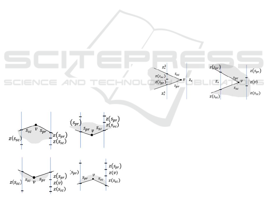
The vertex event changes a set of zones in the
status. These changes are uniquely determined
depending on the type of vertex with which the
event is associated. Variants of this status
transformation are described below for all types of
vertices shown in Fig.5. The "Input" line shows a
fragment of the status before the event, and the
"Output" line shows the same fragment after the
event.
Left Convex Vertex
Site-point v falls into the outer zone 𝑧
∗
. Since the
direction of traversal of the polygon is such that the
interior of the PF lies to the left, in this case the
segment site 𝑠

lies above the segment site 𝑠

. As a
result of processing the event, the 𝑧
∗
zone is split
into two outer zones, and a new inner section is
generated between them, which consists of two new
zones with generator sites 𝑠

and 𝑠

. The result of
the status conversion looks like this (Fig.6a):
Figure 6: Left vertex event (a) convex, (b) concave.
(
a
)
(
b
)
(
c
)
(
d
)
(f)
(g)
(h)
(
e
)
(a)
Before
After
z
∗
𝑠

𝑠

𝑧
∗

𝑧
∗

𝑧
(
𝑠

)
𝑧𝑠


𝑣
After
𝑧

(𝑠)
𝑧
∗
𝑧

(𝑠)
𝑧(𝑠)
𝑧

(
𝑣
)
𝑧

(
𝑣
)
𝑧𝑠


𝑧
(
𝑠

)
𝑠

𝑠

𝑣
(b)
B
e
f
ore
Before
VISAPP 2023 - 18th International Conference on Computer Vision Theory and Applications
438

Input:…,𝑧
∗
,…
Output:…,𝑧
∗

,𝑧
(
𝑠

)
,𝑧𝑠

,𝑧
∗

,…
One new pair of neighboring zones
𝑧
(
𝑠

)
,𝑧𝑠

 is formed.
Left Concave Vertex
The point site 𝑣 falls into the inner section in one of
the zones 𝑧
(
𝑠
)
with the site-generator 𝑠. As a result
of processing the event, the zone 𝑧
(
𝑠
)
is split into
two zones 𝑧

(
𝑠
)
and 𝑧

(
𝑠
)
having the same
generator site 𝑠. And between 𝑧

(
𝑠
)
and 𝑧

(
𝑠
)
a
chain of five new zones is generated and inserted.
One of them is zone is external zone is 𝑧
∗
, it lies
inside the hole of PF. Two zones have a generator
site 𝑣 and in two zones segment sites 𝑠

and 𝑠

are
generators (Fig. 6b).
Input:…,𝑧
(
𝑠
)
,…
Output:
…,𝑧

(
𝑠
)
,𝑧

(
𝑣
)
,𝑧𝑠

,𝑧
∗
,𝑧
(
𝑠

)
,𝑧

(
𝑣
)
,𝑧

(
𝑠
)
,…
Four new pairs of neighboring zones are formed
here:

𝑧

(
𝑠
)
,𝑧

(
𝑣
)

, 𝑧

(
𝑣
)
,𝑧𝑠

,

𝑧
(
𝑠

)
,𝑧

(
𝑣
)

,

𝑧

(
𝑣
)
,𝑧

(
𝑠
)

.
The zone 𝑧
(
𝑠
)
is split into two parts 𝑧

(
𝑠
)
and
𝑧

(
𝑠
)
, which inherit the neighborhood of 𝑧
(
𝑠
)
from
above and below.
Intermediate Convex Vertex
In the case of an intermediate vertex 𝑣, SL intersects
the left site-segment incident to 𝑣, before 𝑣. This is
one of the adjacent 𝑠

or 𝑠

segment sites,
depending on the orientation of the polygon. The
transformation depends on the location of the
polygon relative to this vertex (higher or lower).
Depending on these factors, two options for
transforming a set of zones are obtained.
Figure 7: Intermediate vertex event: (c) upper convex, (e)
lower convex, (f) upper
concave, (d) lower concave.
Vertex 𝑣 is upper convex (Fig. 7c):
Input:…,𝑧
(
𝑠

)
,…
Output:…,𝑧
(
𝑠

)
,𝑧𝑠

,…
Vertex 𝑣 is lower convex (Fig. 7e):
Input:…,𝑧𝑠

…
Output:…,𝑧𝑠

,𝑧
(
𝑠

)
,…
In both cases shown in Fig. 7c and 7e, one new
pair of neighboring zones 𝑧𝑠

,𝑧
(
𝑠

)
 is formed.
Intermediate Concave Vertex
Similar to the case of a convex vertex, this
transformation depends on whether the polygon is
above or below the vertex. There are two options for
transforming the sequence of zones:
Vertex 𝑣 is upper concave (Fig.7f):
Input:…, 𝑧
(
𝑠

)
,…
Output:…, 𝑧
(
𝑠

)
, 𝑧(𝑣), 𝑧𝑠

,…
Vertex 𝑣 lower concave (Fig. 7d):
Input:…, 𝑧𝑠

,…
Output:…, 𝑧
(
𝑠

)
, 𝑧(𝑣), 𝑧𝑠

,…
In both cases, in Fig. 7f and 7d, two new pairs of
neighboring zones are formed: { 𝑧
(
𝑠

)
, 𝑧(𝑣)},
{ 𝑧(𝑣), 𝑧𝑠

}.
Right Convex Vertex
The transformation consists in deleting two zones of
segment sites and "splicing" the two external zones
(Fig. 8g).
Input:…,𝑧
∗

,𝑧𝑠

,𝑧
(
𝑠

)
,𝑧
∗

,…
Output:…,𝑧
∗
,…
In this case, no new pairs of adjacent zones are
formed.
(
g
)
(
h
)
Figure 8: Right vertex events: (g) convex, (h) concave.
Right Concave Vertex
There is a “replacement” of the external zone by
a zone with a generator site 𝑣 (Fig. 8h).
Input:…,𝑧
(
𝑠

)
,z
∗
,𝑧𝑠

,…
Output:…,𝑧
(
𝑠

)
,𝑧
(
𝑣
)
,𝑧𝑠

,…
Two new pairs of adjacent zones are formed:

𝑧
(
𝑠

)
,𝑧
(
𝑣
)

, 𝑧
(
𝑣
)
,𝑧𝑠

.
The analysis of vertex events shows that they
lead to a correction of the status by the generation of
up to five new zones. These zones are inserted into
the status directly one after the other in a known
sequence. In this case, up to four new pairs of
adjacent zones are formed. Each pair of adjacent
zones corresponds to a VD edge. It is necessary to
calculate the endpoints of an edge in order to
construct this edge explicitly. These endpoints are
the vertices of the VD.
(c)
(e)
(f)
(d)
Fast Skeletons of Handwritten Texts in Digital Images
439

6 CLOSURE OF ZONES
In the geometric graph of the VD PF there are
vertices of the first, second and third degree.
Vertices of the first and second degree are points on
the boundary of the PF. The convex PF vertices have
degree 1 in the VD, and the concave vertices have
degree 2. These vertices are formed when the vertex
event occurs.
The VD vertex of the third degree is the internal
point of the PF belonging to three loci. Such a point
is the center of an inscribed circle tangent to the
three sites. The generation of these VD vertices is
associated with the so-called circle events.
A new zone after birth is placed in a status where
it can form new triplets of neighboring zones with
other zones. The number of such new triples can be
from 0 to 3. If it is possible to build a tangent circle
for the site-generators of a triple of neighboring
zones, then its center can turn out to be the vertex
point of the VD. But this will happen if this circle is
"empty", i.e. PF sites lying to the right of the SL will
not fall inside this circle. This cannot be checked at
the moment the circle is formed, but when the SL
moves to the right so that the entire circle is in the
left half-plane, such a check should be made. The
corresponding event, when the SL becomes tangent
to the circle on the right, is called the circle event.
When this event occurs, the middle zone from the
three neighboring zones disappears and is excluded
from the status.
When generating a new zone in the status, it is
necessary to check the condition for the existence of
common tangent circles for triples of site generators
of the resulting new triples of neighboring zones.
The calculation of the tangent circle of three sites is
carried out by the methods of computational
mathematics based on the solution of a system of
equations or by geometric methods, for example,
based on the intersection of bisectors (Marsden,
2020). If such a circle exists, then the center point of
this circle is a candidate for declaring it the vertex of
the VD. We need to schedule a circle event for this
circle. Further, when this event occurs, the point
center of the circle is declared the vertex of the VD.
The circle event leads to the disappearance and
exclusion from the status of one zone. The middle
zone is removed from the triple that defines the
circle.
An illustration of the sequence of events and
changes occurring in the status is shown in Fig.9.
Here PF is a quadrilateral with segment sites
𝑠

,𝑠

,𝑠

,𝑠

. The vertex events are associated with
SL positions labeled A, B, C, G.
The inscribed circle of generator sites 𝑠

,𝑠

,𝑠

is
formed for the three neighboring zones
𝑧(𝑠

),𝑧(𝑠

),𝑧(𝑠

) at position B. This circle is shown
in blue. When it is generated, a circle event is
created, tied to position F. Further, in position C the
zone 𝑧(𝑠

) is included into the status. As a result, a
new triplet of adjacent zones 𝑧(𝑠

),𝑧(𝑠

),𝑧(𝑠

) is
formed. There is an inscribed circle for sites
𝑠

,𝑠

,𝑠

, for which a circle event D is created. This
event is tied to the middle zone of the triple 𝑧(𝑠

).
When the event D occurs, the zone 𝑧(𝑠

)
degenerates into a point and is removed from the
status. Then a new triplet of adjacent zones
𝑧(𝑠

),𝑧(𝑠

),𝑧(𝑠

) appears after its removal. We
build a circle for their site-generators and generate a
circle event at time E. This event is tied to the
middle zone 𝑧(𝑠

) of the triple. Since this zone was
previously tied to a blue circle, events are being
rescheduled. Event F is deleted along with the circle
attached to it, and a new circle event E is scheduled
for the zone 𝑧(𝑠

).
Figure 9: Quad sweeping, vertex events - A, B, C, G, circle
events D, E, F. The composition of the zones is presented
as a result for each event.
The vertex and circle events fully describe the
process of obtaining edges and vertices of the VD
during sweeping.
7 DATA STRUCTURES AND
THEORETICAL COMPLEXITY
The algorithmic paradigm of SL is based on two
data structures: List of events and Status of SL
(Preparata, 1985). In the proposed algorithm, the list
of events is presented in the form of a “priority
queue” data structure, which is effectively
𝑧
(
𝑠

)
𝑧
(
𝑠

)
𝑧
(
𝑠

)
𝑧
(
𝑠

)
𝑧(𝑠

)
𝑧(𝑠

)
𝑧(𝑠

)
𝑧(𝑠

)
𝑧(𝑠

)
𝑧
∗
𝑧(𝑠

)
𝑧(𝑠

)
𝑧(𝑠

)
𝑧(𝑠

)
𝑧(𝑠

)
B
C
D
A
E
G
𝑠

𝑠

𝑠

𝑠

F
VISAPP 2023 - 18th International Conference on Computer Vision Theory and Applications
440

implemented using an AVL tree (a self-balancing
binary search tree). The list of events includes vertex
events and circle events. The total number of events
for an PF with n vertices is 𝑂(𝑛), and the
complexity of processing one event is 𝑂(𝑙𝑜𝑔 𝑛).
A SL Status is a Dictionary structure that
supports insertion, deletion, lookup, and neighbor
selection for an ordered set of zones on a SL. The
standard implementation of this structure based on
the AVL tree is unable to take into account two
features of the dynamic set of zones. Firstly, zones
are inserted into the status in most cases not one at a
time, but in batches of up to 5 zones at the same
time. Secondly, all zones in one package have zero
sizes at birth, i.e. are points on the SL that have the
same ordinate. Therefore, it is necessary to insert the
entire package of zones in one operation in a given
sequence, as shown above in section 5. To solve this
problem, it is proposed to implement the Status
using a combination of a list of zones and an AVL
tree of monotonous border branches described in
section 2 and shown in Fig.3.
The list contains a set of zones ordered from
bottom to top. The operations of inserting and
deleting zones in the list are performed in constant
time, if the place of insertion or deletion is known.
In the case of the events "Passing vertex" and "Right
vertex" this place is a zone of this vertex or of
incident sites-segments. Thus, the processing of
these events is performed in constant time.
For the "Left vertex" event, the insertion place is
not known in advance, it must be determined based
on the localization of this vertex in the current set of
zones. The list makes it possible to do this only by
sequential testing of zones. This operation has linear
complexity in the number of zones. Since the
number of zones in the state and the number of left
vertices in the PF is 𝑂(𝑛), the localization of all left
vertices in the list has complexity 𝑂(𝑛

), which is
unacceptable.
It is proposed to localize the left vertex in two
stages: first, find the section in which the vertex is
located, and then find the required zone in this
section. The AVL-tree of monotone branches
crossing the SL is used to search for a section (Fig.
3). The branches are ordered from bottom to top at
the point of events, each pair of neighboring
branches defines a section of the SL. This structure
defines the section where the left vertex is located.
Since the number of sections is 𝑂(𝑛), finding a
section for a single vertex has 𝑂(𝑙𝑜𝑔 𝑛) complexity.
The search for the zone for the left vertex is
performed on the found section. The section
boundaries are defined by a pair of branches - upper
and lower. And the branches have links to adjacent
zones in the list, so the upper and lower zones of
each section are known.
Further localization of the left vertex requires
checking all zones of the section. For this purpose,
the "fork" algorithm is proposed. The idea of the
algorithm is to check the zones alternately from two
edges inside the section.
Assume that the site contains k zones 𝑧

,…,𝑧

.
The pair (𝑧

,𝑧

) defines the lower and upper
zones of the search interval. First 𝑧

= 𝑧

, 𝑧

=
𝑧

. Let's also designate z.𝑎𝑏𝑜𝑣𝑒 and 𝑧.𝑢𝑛𝑑𝑒𝑟 the
zones in the status, located above and below the
zone 𝑧.
The search for the zone containing the left vertex
𝑣 is carried out iteratively, each iteration includes
two checks:
if the vertex 𝑣 is located in the zone 𝑧

, then
𝑧

is returned, otherwise the search interval is
compressed from below 𝑧

=𝑧

.𝑎𝑏𝑜𝑣𝑒;
if the vertex 𝑣 is located in the zone 𝑧

, then
𝑧

is returned, otherwise the search interval is
compressed from above, 𝑧

=𝑧

.𝑢𝑛𝑑𝑒𝑟.
This iterative process is guaranteed to end
successfully, since the vertex v necessarily falls into
one of the zones in this section. The computational
complexity of the search will be 𝑂(𝑘). In this case,
the maximum number of checks 𝑘 will be required
in the case when the vertex 𝑣 lies in the median zone
𝑧

, 𝑡=


, which occupies the middle position in
the section.
Let us show that the localization of all left
vertices in the zones of the SL has complexity
𝑂(𝑛 𝑙𝑜𝑔 𝑛 ). The number of zones generated during
sweeping is O(n). Without loss of generality, we
assume that there are exactly 𝑛 zones. Let 𝑚 be the
number of left vertices of the PF 𝑚=𝑂(𝑛). Let us
estimate the maximum number of checks for the
entire time of operation. When the “left vertex”
event occurs, the maximum number of checks will
be required if two conditions are met:
• the vertex is localized in the section with the
largest number of zones,
• when localized on the section, the vertex falls
into the median zone, that is, 𝑘 checks are
performed.
Thus, if the maximum number of checks is
always performed, then 𝑛 checks are made for the
first left vertex in a section of 𝑛 zones. After the
formation of new zones associated with the vertex
event, two new sections are formed that will contain


zones each. Two subsequent localizations with the
Fast Skeletons of Handwritten Texts in Digital Images
441

maximum number of checks in segments of length


will require


checks each.
Inserting the corresponding zones into the status
forms four sections of


zones, and so on. At each j-
th level, 2

sections of



zones each are formed.
On these sections, 2

localizations of left vertices
occur with a total number of checks 𝑛. For j levels,
1+2+4+⋯+2

=2

−1 “left vertex” events
are processed. With 𝑗=log
(
𝑚+1
)
we get that all
left vertices can be processed in j levels, since there
are only 𝑛 checks at each level, we get the total
number of checks 𝑂(𝑛 𝑙𝑜𝑔 𝑚 ). Since 𝑚=𝑂(𝑛),
we get the final complexity 𝑂(𝑛 𝑙𝑜𝑔 𝑛).
Thus, the proposed algorithm using the two-
stage hierarchical status of the SL has asymptotic
complexity 𝑂(𝑛 𝑙𝑜𝑔 𝑛).
8 EXPERIMENTS
Practical verification of the algorithm for
correctness, efficiency and reliability uses a set of
polygonal figures of varying complexity: up to 6400
polygonal contours and up to 185,000 polygon
vertices in one binary image. Working time on large
examples is up to 1-1.5 sec.
Efficiency was tested by comparing the running
time of the proposed algorithm and the Fortune's
algorithm from the C++ Boost library
https://www.boost.org/. This algorithm does not take
into account the mutual arrangement of points and
segments in a polygons, and also builds a VD on the
entire plane, and not just for the inner part of the PF.
The comparison of the two algorithms was
carried out in the same environment under the same
conditions. The time was averaged over 10
measurements. On images of a small size (up to
5000 vertices), the algorithm from Boost loses to the
proposed algorithm by 2-4 times, on large images,
with more than 100 thousand vertices, the running
time of the algorithms differs by about 50 times.
Experiments with digital images of a
handwritten text of the type presented in Fig. 2
required about 1 second to build the skeleton.
9 CONCLUSIONS
The article presents an algorithm for constructing an
internal VD PF, focused on practical software
implementation and applications to large-scale
problems, in particular, to work with large images of
handwritten documents. Due to the fact that the VD
is built only for the internal part of the PF, several
useful properties of the algorithm are achieved,
which contribute to an increase in computational
efficiency and numerical reliability.
The concept of the algorithm is based on the
sweeping paradigm used in Fortune's algorithm. The
proposed algorithm implements the reduction of the
problem to the construction of VD linear segments,
but at the same time includes new elements focused
on using the properties of segments made up of
polygons. Due to this, a significant part of the
operations that have logarithmic complexity in the
classical Fortune algorithm is implemented in
constant time. In addition, the amount of
calculations present in the known algorithms that
build the redundant external part of the VD PF is
reduced.
The algorithm has a high numerical reliability,
since the internal VD PF does not require the
calculation of large inscribed circles, as well as
finding the VD vertices located at a very large
distance from the figure.
The proposed algorithm is implemented in full
and is used in solving practical problems of analysis
and recognition of digital images of handwritten
texts.
ACKNOWLEDGEMENTS
This work was supported by the Russian Foundation
for Basic Research, grant no. 20-01-00664, and the
Russian Science Foundation, grant no. 22-68-00066.
REFERENCES
Bae, S.W., (2015). An Almost Optimal Algorithm for
Voronoi Diagrams of Non-disjoint Line Segments.
Lecture Notes in Computer Science, vol. 8973.
Springer, Cham., 34-43.
Fortune S., (1987). A sweepline algorithm for Voronoi
diagrams. Algorithmica, 2, 153 - 174
Held M., (2001). Vroni: An engineering approach to the
reliable and efficient computation of Voronoi
diagrams of points and line segments. Computational
Geometry, vol. 18, p. 95–123,
Imai T., (1996). A topology oriented algorithm for the
Voronoi diagram of polygons. cccg1996, pp.107–112
Lee D.T., (1982). Medial axes transform of planar shape //
IEEE Trans. Patt. Anal. Mach. Intell. PAMI-4. –– p.
363–369.
Marsden, Daniel, (2020). Exact Generalized Voronoi
Diagram Computation using a Sweepline Algorithm.
VISAPP 2023 - 18th International Conference on Computer Vision Theory and Applications
442

All Graduate Theses and Dissertations. 7947.
https://digitalcommons.usu.edu/etd/7947
Menelaos I. Karavelas., (2004). A robust and efficient
implementation for the segment Voronoi diagram.
In Proc. Internat. Symp. on Voronoi diagrams in
Science and Engineering (VD2004), p. 51–62.
Mestetskiy L., Semenov A., (2008). Binary image skeleton
continuous approach, VISAPP 2008 - 3rd Int. Conf. on
Comp. Vis. Theory and App., Proceeding, Funchal,
Madeira, vol.1, p. 251-258
Preparata, F.P. and Shamos, M.I., (1985). Computational
Geometry. Springer, Berlin.
Sugihara, K., Iri, M., Inagaki, H. et al., (2000), Topology-
Oriented Implementation—An Approach to Robust
Geometric Algorithms. Algorithmica 27, p. 5–20.
Srinivasan V. and Nackman L. R. (1987). Voronoi
diagram for multiply-connected polygonal domains I:
Algorithm, in IBM Journal of Research and
Development, vol. 31, no. 3, p. 361-372, May 1987.
Fast Skeletons of Handwritten Texts in Digital Images
443