Compression of GPS Trajectories Using Autoencoders

Michael K

olle, Steffen Illium, Carsten Hahn, Lorenz Schauer, Johannes Hutter

and Claudia Linnhoff-Popien

Institute of Informatics, LMU Munich, Oettingenstraße 67, Munich, Germany

ﬁ

Keywords:

Trajectory Compression, Autoencoder Model, LSTM Networks, Location Data.

Abstract:

The ubiquitous availability of mobile devices capable of location tracking led to a signiﬁcant rise in the col-

lection of GPS data. Several compression methods have been developed in order to reduce the amount of

storage needed while keeping the important information. In this paper, we present an lstm-autoencoder based

approach in order to compress and reconstruct GPS trajectories, which is evaluated on both a gaming and

real-world dataset. We consider various compression ratios and trajectory lengths. The performance is com-

pared to other trajectory compression algorithms, i.e., Douglas-Peucker. Overall, the results indicate that our

approach outperforms Douglas-Peucker signiﬁcantly in terms of the discrete Fr

echet distance and dynamic

time warping. Furthermore, by reconstructing every point lossy, the proposed methodology offers multiple

advantages over traditional methods.

1 INTRODUCTION

The rising popularity of modern mobile devices such

as smartphones, tablets or wearables and their now

ubiquitous availability led to a vast amount of col-

lected data. Additionally, such devices can determine

the user’s current location and may offer position-

tailored information and services. However, resource

(energy) limitations apply. In contrast to energy sav-

ing, embedded systems, smartphones are typically at

the upper hardware limit. When dealing with GPS

information, the data analysis is being outsourced to

data centers, often. A common way to transmit the

data from the mobile devices to central servers is via

cellular or satellite networks. According to Meratnia

and de By (Meratnia and de By, 2004), around 100Mb

of storage size are needed, if just 400 objects col-

lect GPS information every ten seconds for a single

day. Considering large vehicle ﬂeets or mobile ap-

plications with millions of users tracking objects for

long time spans, it is obvious that there is a need to

optimize the transmission and storage of trajectories

through compression.

In this paper, we investigate and evaluate the ap-

proach of autoencoders for compression and recon-

struction of GPS trajectories. For evaluation, we iden-

tify adequate distance metrics that measure the sim-

ilarities between trajectories to evaluate the method

and compare it to existing handcrafted compression

algorithms, such as Douglas-Peucker. As main con-

tribution, we will answer the following research ques-

tions:

1) How well does an autoencoder model perform in

trajectory compression and reconstruction compared

to traditional line simpliﬁcation methods?

2) How well does an autoencoder model perform for

different compression ratios and different trajectory

lengths?

The paper is structured as follows: Section 2 holds

related work. Section 3 presents our methodology.

Evaluation is done in Section 4, and ﬁnally, Section 5

concludes the paper.

2 RELATED WORK

A common method to compress (2-dimensional) tra-

jectories are line simpliﬁcation algorithms, such as

the Douglas-Peucker (Douglas and Peucker, 1973). In

contrast, GPS trajectories include time as an impor-

tant third dimension. To overcome this misconcep-

tion, Meratnia and de By (Meratnia and de By, 2004)

state that the propose a variant called Top-Down Time-

Ratio (TD-TR) using the synchronized Euclidean dis-

tance (SED) as error metric. Beside line simpliﬁca-

tion, road network compression is applied in litera-

ture. Kellaris et al. (Kellaris et al., 2009) combine

GPS trajectory compression with map-matching us-

Kölle, M., Illium, S., Hahn, C., Schauer, L., Hutter, J. and Linnhoff-Popien, C.

Compression of GPS Trajectories Using Autoencoders.

DOI: 10.5220/0011782100003393

In Proceedings of the 15th International Conference on Agents and Artiﬁcial Intelligence (ICAART 2023) - Volume 3, pages 829-836

ISBN: 978-989-758-623-1; ISSN: 2184-433X

 2023 by SCITEPRESS – Science and Technology Publications, Lda. Under CC license (CC BY-NC-ND 4.0)

829

ing TD-TR. Richter et al. (Richter et al., 2012) ex-

ploit the knowledge about possible movements with

the use of semantic trajectory compression (STC).

The COMPRESS framework, introduced by Han et

al. (Han et al., 2017), relies on knowledge about the

restricted paths an object can move on. Chen et al.

(Chen et al., 2013) exploit the existence of repeated

patterns and regularity in trajectories of human move-

ment by extracting so-called pathlets from a given

dataset.

The main focus of autoencoder research in recent

years has been on the compression of image data,

such as (Gregor et al., 2016). Oord et al. (van den

Oord et al., 2016) introduced PixelRNN, a genera-

tive model allowing the lossless compression of im-

ages with state-of-the-art performance. The approach

is based on (Theis and Bethge, 2015) where two-

dimensional LSTM networks are proposed to model

the distributions of images. Toderici et al. (Toderici

et al., 2015) use a combination of LSTM and CNN

elements to compress thumbnail images. It is suitable

for small images but falls behind manually composed

algorithms for larger resolutions. This downside is

partially overcome in the subsequent work (Toderici

et al., 2016) where an average performance better than

JPEG can be achieved. Masci et al. (Masci et al.,

2011) propose a deep autoencoder based on CNN.

The introduced convolutional autoencoder (CAE) is

trained layer-wise and the resulting weights are used

as a pre-training for a classiﬁcation network. Rippel

and Bourdev (2007) improve on the aforementioned

methods and suggest a generative adversarial network

(Rippel and Bourdev, 2017). The authors claim to

double the compression ratio compared to JPEG and

WebP while reaching the same quality. Beside im-

age compression, autoencoders are applied for differ-

ent purposes. E.g. Testa and Rossi (2015) use an au-

toencoder to compress biomedical signals (Testa and

Rossi, 2015).

Overall, there is only few research dealing with

the compression of time series data using autoen-

coders.There is a combination of LSTM and autoen-

coder to compress a seismic signal (Hsu, 2017). Sim-

ilarly, Hejrati et al. compress electroencephalogram

data with a multi-layer perceptron (Hejrati et al.,

2017).

3 METHODOLOGY

In this section, we introduce our methodology for tra-

jectory compression. Since the trajectory of a moving

object is usually represented as a time series of dis-

crete positions annotated with a timestamp, an RNN is

used to build the autoencoder’ model. More precisely,

an LSTM network architecture is applied, due to its

remarkable performance in classiﬁcation and predic-

tion tasks with time series data.

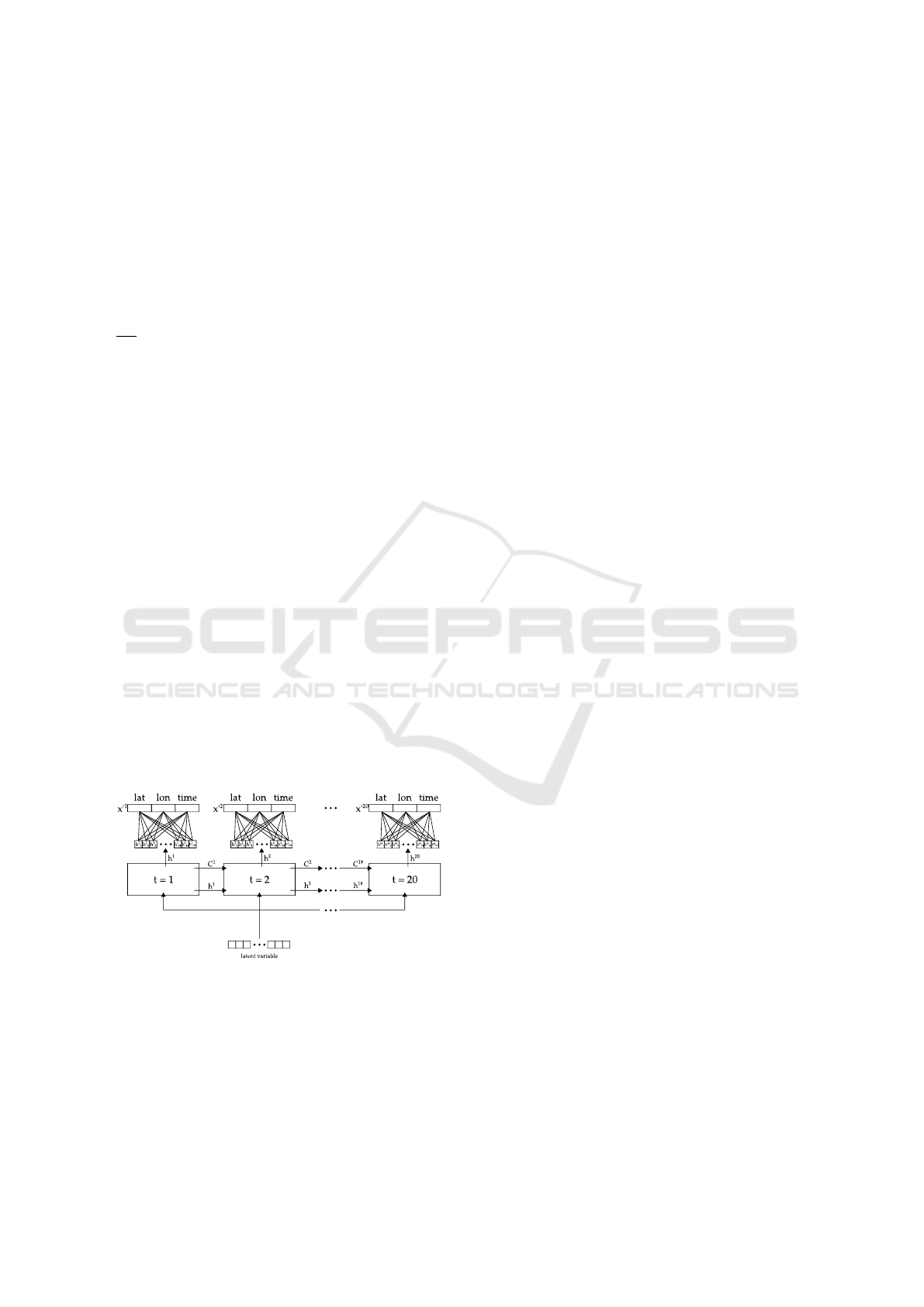
3.1 Encoder

Figure 1: Schematic of the LSTM encoder.

As already stated, the encoder part transforms the in-

put trajectory into a lower-dimensional latent repre-

sentation. At each time step a data point of the trajec-

tory is fed to and processed by the LSTM. Depending

on the used dataset, the three dimensions represent

the position of an object inside a three-dimensional

space or a two-dimensional position and a timestamp,

respectively. To reduce complexity, the length of the

trajectory |T | is ﬁxed beforehand. The output at ev-

ery time step, but the last, is discarded as the ﬁnal

output contains the encoded information of the whole

trajectory including the temporal dependencies. This

latent representation forms together with the scaling

and offset value from the normalization step the com-

pressed version of the original trajectory. Per trajec-

tory and feature two rescaling values for absolute po-

sition and scaling factor are needed so that six val-

ues are already set for the compressed trajectory. The

number of values in the original trajectory are |T | · 3,

since there are three values for each point in the tra-

jectory. All the points of the trajectories as well as the

rescaling values and the latent variable of the autoen-

coder are stored in 32 bit each, so that the number of

values in the original and compressed representation

can be directly used to calculate the compression ra-

tio. Since the size of an input trajectory and the size

of the rescaling values are set, the compression ratio

can be adjusted by modifying the dimensionality of

the encoder’s output and therefore the latent variable

of the autoencoder. The compressed size is the sum

of the numbers of latent and rescale values. Figure 1

depicts our LSTM encoder mapping a trajectory into

the latent space.

3.2 Decoder

Our decoder consists of a LSTM cell. At each time

step the latent variable is fed again to the network as

its input and the corresponding output represents the

reconstructed three-dimensional data point. During

the training process the weights are optimized in or-

ICAART 2023 - 15th International Conference on Agents and Artiﬁcial Intelligence

830

der to produce the expected output and learn gener-

alizable features of the given data. Hence, the perfor-

mance depends on the amount of weights which is de-

pendent on the dimensionality of the input and output

data. Since the weights are reused at each time step,

the sequence length does not inﬂuence the amount.

Compared to other tasks, such as image compression

or natural language generation, the spatio-temporal

data we use is low-dimensional, e.g., with a sequence

length of 20 and a compression ratio of 4 we deal with

20·3

= 15 dimensions. Due to 2 × 3 variables for off-

set and scaling factor from the normalization step, the

latent variable is of 15 - 6 = 9 dimensions. Hence,

the input size of the decoder at each time step is 9,

while the output size is 3. The number of weights n

available in the cell depends on the amount of neu-

ral layers. In a LSTM cell, gates are implemented as

neural layers and the block input as well as the output

is activated by a layer. The number of weights can

therefore be calculated by:

= 4 · ((n

+ 1) · n

+ n

)

where n

is the input, and n

the output dimension-

ality. The additional 1 is due to the bias term. The

factor 4 represents the three gates of a LSTM and the

input activation. In the example, the decoder would

have 156 weights available to ﬁt to the data. This is

insufﬁcient for a complex task, such as trajectory re-

construction. Hence, we set the output dimensionality

of the decoder to 100 in order to deal with enough pa-

rameters that can be adjusted to ﬁt the temporal de-

pendencies between points. In order to reduce the

output back to a three dimensional space, a fully con-

nected layer with three output neurons is added at the

LSTM output. Figure 2 depicts our architecture of the

decoder.

Figure 2: Schematic of the LSTM decoder.

Sutskever et al. (Sutskever et al., 2014) stated that

the performance of Sequence to Sequence Autoen-

coders can be improved signiﬁcantly, if the input se-

quence is reversed before it is fed to the network. The

target sequence stays in the original order nonethe-

less. While no ﬁnal explanation for this phenomenon

could be provided, the assumption is, that the intro-

duction of more short-term dependencies enables the

network to learn signiﬁcant features. Hence, we apply

this method to our proposed model.

3.3 Training Loss

Autoencoders are usually trained with the mean

squared error (MSE) as loss function. The values

of input and output can therefore be compared in a

value-by-value fashion. Nonetheless MSE is a gen-

eral metric that doesn’t incorporate domain knowl-

edge in its error computation. If the temporal dimen-

sion is only implicitly available through a ﬁxed sam-

pling rate, solely the reconstruction of the spatial in-

formation is important. In this case, the Euclidean

distance between a point and its reconstruction suf-

ﬁces as loss metric.

Trajectories fed to and reconstructed by a neural

network are however normalized. If the Euclidean

loss is computed on normalized trajectories, the ac-

tual distances are hidden. Hence, the training step can

be further improved by rescaling the original and re-

construction before loss calculation.

When working with GPS data, trajectories are rep-

resented in geo-coordinates annotated with a times-

tamp. The temporal information is therefore explic-

itly available. Hence, an error calculation based on

the Euclidean distance would be inaccurate. In this

case, the haversine distance would be more general,

more accurate and more expressive. However, the

computation is way more expensive than the Eu-

clidean distance, while the equirectangular approxi-

mation offers a trade-off between both. Therefore, we

consider this approximation to calculate the distance

between expected and predicted points. To incorpo-

rate the time in the loss function, the squared error of

this dimension is added to the loss.

4 EVALUATION

4.1 Datasets and Preprocessing

For evaluation, we consider two datasets consisting of

multiple recorded trajectories but varying in structure

and origin as follows:

Quake III Dataset: consists of trajectories recorded

in Quake III Arena, a popular ﬁrst-person shooter

video game (Breining et al., 2011). The player is able

to move inside a ﬁxed three dimensional area produc-

ing a series of three-dimensional positions. This lo-

cation data is recorded at each position update which

takes place every 33 ms - based on an frame rate of

30 fps. The sampling rate here is therefore far higher

Compression of GPS Trajectories Using Autoencoders

831

than in real life scenarios. Furthermore, and in con-

trast to real positioning systems, there is no position-

ing error in the recorded location data. Temporal in-

formation is represented only implicitly through the

ﬁxed sampling rate and accessible relatively to the

start of the trajectory. The data was recorded in dif-

ferent scenarios and settings. Each run represents a

trajectory from spawn to death. Since this dataset is

recorded directly from the game, the level of accuracy

is high and there is no need for further preprocessing

steps.

T-Drive: The original T-Drive dataset (Yuan et al.,

2010) contains recorded trajectories of about 33,000

taxis in Beijing over the course of three months. We

use the public part containing more than 10,000 taxi

trajectories over the course of one week resulting in

15 million sample points. Each point contains a taxi

ID, a timestamp and the position of the car in lati-

tude/longitude representation. The duration between

two samples lasts from few seconds to multiple hours.

Due to inaccurate or faulty GPS-samples, there are in-

consistencies in this dataset which should be removed

in a preprocessing step. Hence, we only consider tra-

jectories which are located in the metropolitan area

of Beijing and show continuously increasing times-

tamps. Idle times should also be removed from the

data since they add no informational value. Based on

speed information, we also remove outliers that are

probably introduced by technical errors. Hence, obvi-

ous inconsistencies are removed by these preprocess-

ing steps, while the level of inaccuracy due to techni-

cal limitations stays realistic.

4.2 Training and Normalization

Both datasets are split into two independent parts:

90% of the recorded points are used for training and

the remaining 10% are used to test and validate the

trained model to avoid overﬁtting effects. Our tra-

jectories consist of varying numbers of time steps.

Hence, we consider different sequence lengths of tra-

jectories, such as |T | = 20 and |T| = 40.

In order to increase the amount of training data,

a sliding window approach is applied. If a trajectory

consists of more time steps than the required sequence

length |T |, the ﬁrst |T | points (P

, ..., P

|T |

) are added

to the training data as input sequence. Afterwards,

the sliding window is shifted by one so that the steps

, ..., P

|T |+1

) build the next input sequence. This

procedure is subsequently repeated until the end of

the trajectory is reached. Through this approach, the

number of sequences to train the model can be en-

larged. The trajectories used for testing are not fur-

ther manipulated but also split into chunks of 20 and

40 steps.

Similarities between trajectories are often based

on the form of the route they describe, rather than

their absolute position in space. Rescaling each tra-

jectory to values between 0 and 1 takes complexity

out of the network leading to better performance and

shorter learning time. For each dimension, the min-

imum value (offset) and the scaling factor of a tra-

jectory are saved. The compressed trajectory there-

fore consists of the output of the encoder network and

the information to rescale the trajectory to its origi-

nal domain. After decoding the latent representation,

the trajectory can be put to its absolute position with

those rescaling and offset values. Thus, the autoen-

coder has to learn the relative distances between the

points of the trajectory, rather than absolute values.

4.3 Implementation and Setup

The encoder was implemented as a plain LSTM cell,

taking as input a mini-batch with a ﬁxed number of

time steps. This decoding LSTM cell has an output

dimensionality of 100 in order to increase the ability

to learn hidden features. As optimizer, we use Adam

(Kingma and Ba, 2014) at default parameters.

Since the sequence length of the input trajecto-

ries is ﬁxed for the autoencoder, it should be eval-

uated, how well the model performs with different

given lengths |T |. Therefore, each experiment is per-

formed once with trajectories containing 20 & 40 data

points. Another important property that has to be

tested is the performance given different compression

ratios (c.p. Table 1). For the autoencoder the number

of compressed values is the sum of the dimensional-

ity of the latent variable and the variables needed for

offset and rescaling. For Douglas-Peucker it is the

product of the number of points of the compression

and their dimensionality.

Comparable compression ratios are limited by two

factors. First, Douglas-Peucker selects a subset of

the original trajectory. Hence, the amount of values

in the compressed trajectory has to be divisible by

3. Second, the proposed autoencoder model transfers

the rescale variables together with the latent variable.

Hence, the number of values in the compressed tra-

jectory has to be greater than 6.

Table 1: Scenarios evaluated for sequence length 40.

Comp. Ratio Autoencoder Douglas-Peucker Comp. Values

2 54 + 6 20 · 3 60

4 24 + 6 10 · 3 30

8 9 + 6 5 · 3 15

10 6 + 6 3 · 3 12

The errors between the original and the com-

pressed/reconstructed trajectories are subsequently

ICAART 2023 - 15th International Conference on Agents and Artiﬁcial Intelligence

832

calculated for the three considered metrics, i.e., mean

Euclidean/Haversine distance, Fr

echet distance, and

DTW. In the following sections, we present the ob-

tained results for both datasets, separately.

4.4 Performance on Quake III Dataset

First, we take the Quake III dataset.

Trajectories of Sequence Length 20. The autoen-

coder reconstructs the intermediate compression back

to the original sequence length of 20 points, while

Douglas-Peucker yields 10, 5 and 3 points, respec-

tively. For the autoencoder reconstruction the mean

Euclidean distance between points can be calculated

intuitively, while the trajectories that are compressed

with Douglas-Peucker have to be interpolated ﬁrst in

order to equalize the sequence lengths. Therefore, re-

moved points are approximated on the line segments

of the compressed trajectory by linear interpolation.

We notice, that the autoencoder performs worse

than Douglas-Peucker for low compression ratio,

which is the opossite for higher compression ra-

tios. We assume, this is due to the way Douglas-

Peuker selects a subset of the original trajectory: For

a compression ratio of 2, half of the points in the

compressed trajectory stay exactly the same. For

higher compression ratios, less points are identical

and the distance becomes higher. The difference be-

tween Douglas-Peucker and the autoencoder is all-in-

all small and the tendency over different compres-

sion ratios is similar. It has to be noted however,

that the approximated locations can’t be interpolated

in this way in a real-life scenario, since the number

of deleted points between the compressed locations

can only be calculated if the original trajectory is still

available. The autoencoder model on the other hand

reconstructs each point of th trajectory. Therefore, the

comparison method favors Douglas-Peucker, but the

autoencoder model still performs better, at least for

higher compression ratios within our settings.

When analyzing the mean discrete Fr

echet dis-

tances, the autoencoder performs signiﬁcantly better

than Douglas-Peucker across all compression ratios.

However, sincethis metric is an approximation of the

actual Fr

echet distance, it is sensitive regarding dif-

ferences in the number of vertices of the compared

polylines. This can also be veriﬁed by interpolating

the deleted points.

We did also compare the interpolated autoen-

coder reconstructions to trajecetories, compressed

with Douglas-Peucker. While the autoencoder per-

forms slightly better in terms of Fr

echet distance for

a compression ratio of 2, it performs worse for the

other two ratios. However, the compressed trajecto-

Table 2: Mean Euclidean distance for sequence length 40

with Quake III dataset.

Comp. Ratio Douglas-Peucker Autoencoder

2 1.45 1.76

4 3.82 3.75

8 14.85 13.88

10 24.87 24.39

Table 3: Mean Fr

echet and DTW distances for sequence

length 40 with Quake III dataset.

Douglas-Peucker

CR Normal Interpolated Autoencoder

echet 30.23 7.89 7.29

DTW 278.40 46.33 70.09

echet 52.45 14.92 16.86

DTW 616.59 117.36 144.79

echet 93.36 41.03 64.98

DTW 1304.55 423.59 509.51

echet 114.63 58.32 87.33

DTW 1701.29 701.62 882.43

ries yielded by Douglas-Peucker had to be enriched

with information from the original trajectory, whereas

the reconstructions from the autoencoder were not

manipulated.

The trajectories considered here consist of three-

dimensional spatial positions. Hence, the consider

DTW

, since the dimensions are dependent of each

other. As explained previously, DTW has similari-

ties to the Fr

echet distance and therefore it is sensitive

to different sequence lengths. We notice similar ten-

dencies in comparison to the discrete Fr

echet errors

from above. The distances regarding the autoencoder

reconstructions are smaller than in case of Douglas-

Peucker compressions without interpolated points.

Trajectories of Sequence Length 40. We evaluate

trajectories with a sequence length of 40 positions.

The higher length also allows higher compression ra-

tios, e.g., 8 and 10. The corresponding results are

shown in Table 2 considering the mean Euclidean dis-

tances as error.

It can be seen, that our previous observations can

be replicated for longer trajectories. The autoencoder

model performs worse for a compression to half of

the original size, while higher compression ratios pro-

duce similar results with a tendency in favor of the

autoencoder. That implies that the temporal depen-

dencies between the points can be captured for both

sequence lengths equally well.

In case of Fr

echet and DTW, the results are also

comparable to the lower sequence lengths, as shown

in Table 3. For a better comparison, the trajectories

Compression of GPS Trajectories Using Autoencoders

833

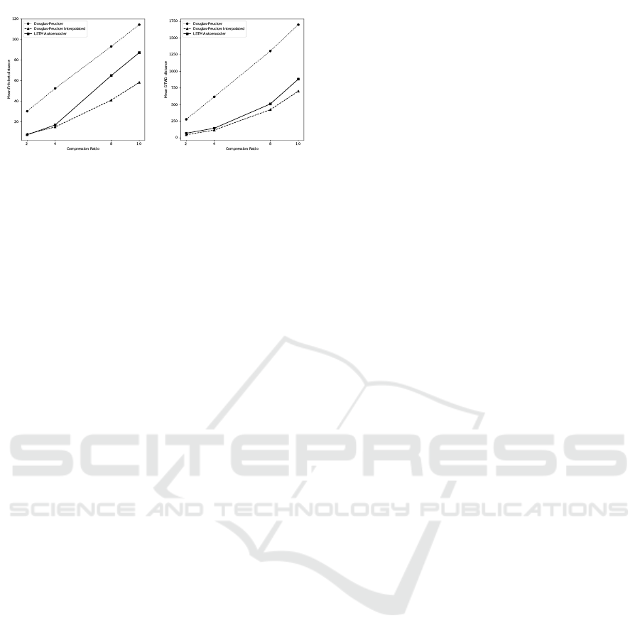
(a) Mean Fr

echet distance. (b) Mean DTW distance.

Figure 3: Mean distances for sequence length 40 and com-

pression ratios 2, 4, 8, 10.

compressed by Douglas-Peucker were again interpo-

lated to the same number of points as the original tra-

jectories. The distances between the originals and the

reconstructions from the autoencoder are far smaller

than the ones between original and Douglas-Peucker

compressions. However, the distances between origi-

nal and interpolated compressions are lower than the

autoencoder errors. Hence, we state that the main ad-

vantage of the autoencoder is the reconstruction of ev-

ery point of the original trajectory in contrast to the

selection of a subset.

Figure 3 shows the mean Fr

echet and DTW dis-

tances for a sequence length of 40 over the four tested

compression ratios. The distances between original

trajectories and their subsets produced by Douglas-

Peucker increase linearly over the compression ratio

for both distance metrics. The Fr

echet distance to the

autoencoder reconstruction is less than the distance

between original and interpolated Douglas-Peucker

compression for a ratio of 2, but for higher ratios the

autoencoder error grows faster. As explained before,

the Fr

echet distance is sensitive to outliers, since it

represents the maximum of the minimal distances be-

tween points. As the distance grows faster for the au-

toencoder, more outliers are produced. This obser-

vation is supported by Figure 3 where the mean DTW

distances are shown. The autoencoder distance here is

always higher than the interpolated Douglas-Peucker

distance, but the difference between both methods

grows slower for higher compression ratios compared

to the Fr

echet distance in Figure 3. Since DTW mea-

sures the sum of minimal distances between points,

this metric is not as sensitive to outliers as the Fr

echet

distance. An explanation for the increased errors in

case of higher compression ratios is the dimensional-

ity of the latent space. With a trajectory of 40 three-

dimensional points and a compression ratio of 10, the

compression contains only 12 values. Six values are

already reserved for rescaling and offset, so that the

latent space has a low dimensionality of 6. Hence, it’s

hard to capture all temporal dependencies.

4.5 Performance on T-Drive Dataset

In contrast to the Quake trajectories, the T-Drive data

points consist of two-dimensional GPS locations and

a temporal annotation. Since the spatial positions are

now represented as latitude/longitude pairs, the haver-

sine distance is used instead of the Euclidean distance

and the error is expressed in meters rather than us-

ing abstract distances like before. In the following,

we evaluate a spatial and a time-synchronized com-

parison separately. During the ﬁrst, we omit temporal

dimension, while for the second, we incorporate tem-

poral information by synchronizing the spatial points

in time before performing distance computations.

4.5.1 Spatial Comparison

In order to see whether the results observed in the

compression of the Quake III dataset can be repro-

duced for real-life data, the temporal component of

the T-Drive dataset is not considered. However, the

compression is done on the whole three-dimensional

trajectories. As in the previous evaluation, the tra-

jectories compressed with Douglas-Peucker are once

considered directly as a subset of the original data

and once with the interpolated approximations of the

deleted points.

We notice, a slighty higher mean haversine error

of the autoencoder than the mean distance to the in-

terpolated compressions of Douglas-Peucker. This is

contrary to the results obtained with 20-point trajec-

tories from the Quake III dataset. However, the differ-

ence between both compression methods stays stable

for all three tested compression ratios. Like in the pre-

vious experiments, the discrete Fr

echet and DTW

error of the autoencoder is signiﬁcantly lower than

the error between original trajectories and the subsets

produced by TD-TR. The DTW

error of the autoen-

coder is however higher than the error of interpolated

TD-TR compressions. The tendency that the autoen-

coder performs better than the interpolated TD-TR

compressions for lower compression ratios in terms

of Fr

echet distance can be replicated for the T-Drive

dataset. Overall, the results are similar and the per-

formance of our model is not dependent on the com-

pressed datasets.

Figure 4 shows the obtained errors for the com-

pression with sequence length 40. The results are

similar to the observations with 20 points per trajec-

tory. This gives again reason for the assertion that the

model performs equally for both sequence lengths.

Furthermore, the results show that the difference be-

tween autoencoder and TD-TR are smaller for higher

compression ratios. This is especially visible for the

mean haversine distance, where the autoencoder per-

ICAART 2023 - 15th International Conference on Agents and Artiﬁcial Intelligence

834

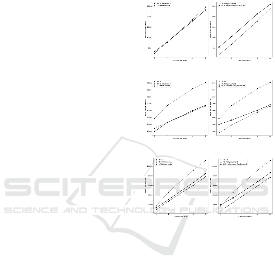
forms better with compression ratios of 8 and 10.

4.5.2 Time-Synchronized Comparison

Since the trajectories compressed with TD-TR are

a subset of the original trajectories, the remaining

points are already synchronized in time. The interpo-

lated compressions and the autoencoder reconstruc-

tions however contain positions that are not synchro-

nized and therefore do not consider the temporal in-

formation. In order to include this additional dimen-

sion in the evaluation, both interpolated TD-TR com-

pressions and autoencoder reconstructions are now

synchronized before error calculation.

We notice, that the performance of both compres-

sion methods differ to our previous observations. For

TD-TR, the errors are lower if the interpolated tra-

jectory is synchronized in time. This is due to the

usage of SED as metric to decide which points are

stored in the compressed version. Considering the

autoencoder, the distances to time-synchronized re-

constructions are higher, especially for low compres-

sion ratios. This indicates, that the accuracy of the re-

constructed temporal dimension is low and hence, the

positions of the synchronized points are further away

from the original positions. An adapted loss function

may improve the accuracy, e.g., by additional weight-

ing the reconstruction error of the timestamp, or cal-

culating a time-synchronized distance.

The results for the time-synchronized error with

a sequence length of 40 are shown in the right col-

umn of Figure 4. Obviously, the results from the 20-

point trajectories and the spatial distances can be re-

produced. The autoencoder performs generally worse

than the synchronized TD-TR compression, but the

difference is smaller for higher compression ratios.

5 CONCLUSION AND FUTURE

WORK

In this paper, we have investigated the feasibility of

an autoencoder approach for GPS trajectory compres-

sion. For this purpose, an LSTM network architec-

ture was developed and evaluated using two diverse

datasets.

The obtained results lead to the conclusion that

reconstructions of the proposed model outperform

Douglas-Peucker compressions signiﬁcantly in terms

of discrete Fr

echet distance and DTW distance. With

equalized sequence lengths through interpolation of

the Douglas-Peucker compressions, our autoencoder

still produces a lower Fr

echet error for low compres-

sion ratios. For high compression ratios, the pro-

(a) Mean haversine distance.

(b) Mean Fr

echet distance.

Figure 4: Mean distances for sequence length 40 and com-

pression ratios 2, 4, 8 and 10 on the T-Drive dataset. Tra-

jectories have been time synchronized on the right side.

posed method achieves better results in terms of mean

point-to-point distances depending on the representa-

tion space of the trajectories. While Douglas-Peucker

selects a subset of the original trajectory, the autoen-

coder approach reconstructs every point lossy. This

conceptual difference between the two methods is an

advantage for the autoencoder if temporal information

of the trajectory is only available implicitly through a

ﬁxed sampling rate. Furthermore, the reconstruction

approach allows a better retention of form and shape

of the trajectory. The performance of the autoencoder

is reproducible for different trajectory lengths as well

as for different datasets. In contrast to most line sim-

pliﬁcation algorithms, the user may ﬁx the compres-

sion ratio before compression, which is advantageous

for use cases where ﬁxed storage or transmission sizes

are expected. However, in terms of DTW distance, the

Compression of GPS Trajectories Using Autoencoders

835

autoencoder approach always performed worse than

Douglas-Peucker if equalized sequence lengths are

considered. Furthermore, the performance was worse

for time-synchronized trajectories.

We summarize, that compressing GPS trajectories

using an autoencoder model is feasible and promis-

ing. The performance of our proposed model could

still be improved by various approaches. First, per-

forming map-matching methods after decoding may

decrease the reconstruction error, if an underlying

road network is present on the decoder side. Sec-

ond, the usage of a stacked autoencoder which feeds

the LSTM outputs at each time step to another LSTM

layer, so that temporal and spatial dependencies are

captured more effectively. Generally, the perfor-

mance can also be increased by using optimized hy-

perparameters and more efforts in training. Lately

variational and adversarial autoencoder have proven

to be successful advancements of normal autoen-

coders. Furthermore, the usage of a more efﬁcient

and differentiable loss function focusing on time se-

ries, such as Soft-DTW (Cuturi and Blondel, 2017),

seems promising to improve our model signiﬁcantly.

In future work, we will enhance our investigations

regarding these approaches. Overall, further research

in this domain is highly promising and the incorpo-

ration of neural networks for trajectory compression

could create a new category next to line simpliﬁcation

and road network-based solutions.

REFERENCES

Breining, S., Kriegel, H., Z

uﬂe, A., and Schubert, M.

(2011). Action sequence mining. ecml/pkdd work-

shop on machine learning and data mining in games.

Chen, C., Su, H., Huang, Q., Zhang, L., and Guibas, L.

(2013). Pathlet learning for compressing and planning

trajectories. In Proceedings of the 21st ACM SIGSPA-

TIAL International Conference on Advances in Geo-

graphic Information Systems, SIGSPATIAL’13, pages

392–395, New York, NY, USA. ACM.

Cuturi, M. and Blondel, M. (2017). Soft-dtw: a differ-

entiable loss function for time-series. arXiv preprint

arXiv:1703.01541.

Douglas, D. H. and Peucker, T. K. (1973). Algorithms for

the reduction of the number of points required to rep-

resent a digitized line or its caricature. Cartograph-

ica: The International Journal for Geographic Infor-

mation and Geovisualization, 10(2):112–122.

Gregor, K., Besse, F., Rezende, D. J., Danihelka, I., and

Wierstra, D. (2016). Towards conceptual compres-

sion. In Lee, D. D., Sugiyama, M., Luxburg, U. V.,

Guyon, I., and Garnett, R., editors, Advances in Neu-

ral Information Processing Systems 29, pages 3549–

3557. Curran Associates, Inc.

Han, Y., Sun, W., and Zheng, B. (2017). Compress: A

comprehensive framework of trajectory compression

in road networks. ACM Transactions on Database

Systems (TODS), 42(2):11.

Hejrati, B., Fathi, A., and Abdali-Mohammadi, F. (2017). A

new near-lossless eeg compression method using ann-

based reconstruction technique. Computers in Biology

and Medicine.

Hsu, D. (2017). Time series compression based on adap-

tive piecewise recurrent autoencoder. arXiv preprint

arXiv:1707.07961.

Kellaris, G., Pelekis, N., and Theodoridis, Y. (2009). Tra-

jectory compression under network constraints. Ad-

vances in Spatial and Temporal Databases, pages

392–398.

Kingma, D. P. and Ba, J. L. (2014). Adam: A method for

stochastic optimization. CoRR, abs/1412.6980.

Masci, J., Meier, U., Cires¸an, D., and Schmidhuber, J.

(2011). Stacked Convolutional Auto-Encoders for Hi-

erarchical Feature Extraction, pages 52–59. Springer

Berlin Heidelberg, Berlin, Heidelberg.

Meratnia, N. and de By, R. A. (2004). Spatiotemporal com-

pression techniques for moving point objects. In In-

ternational Conference on Extending Database Tech-

nology, pages 765–782. Springer.

Richter, K.-F., Schmid, F., and Laube, P. (2012). Seman-

tic trajectory compression: Representing urban move-

ment in a nutshell. Journal of Spatial Information Sci-

ence, 2012(4):3–30.

Rippel, O. and Bourdev, L. (2017). Real-time adaptive im-

age compression. arXiv preprint arXiv:1705.05823.

Sutskever, I., Vinyals, O., and Le, Q. V. (2014). Sequence to

sequence learning with neural networks. In Ghahra-

mani, Z., Welling, M., Cortes, C., Lawrence, N. D.,

and Weinberger, K. Q., editors, Advances in Neu-

ral Information Processing Systems 27, pages 3104–

3112. Curran Associates, Inc.

Testa, D. D. and Rossi, M. (2015). Lightweight lossy com-

pression of biometric patterns via denoising autoen-

coders. IEEE Signal Processing Letters, 22(12):2304–

2308.

Theis, L. and Bethge, M. (2015). Generative image model-

ing using spatial lstms. In Cortes, C., Lawrence, N. D.,

Lee, D. D., Sugiyama, M., and Garnett, R., editors,

Advances in Neural Information Processing Systems

28, pages 1927–1935. Curran Associates, Inc.

Toderici, G., O’Malley, S. M., Hwang, S. J., Vincent, D.,

Minnen, D., Baluja, S., Covell, M., and Sukthankar,

R. (2015). Variable rate image compression with re-

current neural networks. CoRR, abs/1511.06085.

Toderici, G., Vincent, D., Johnston, N., Hwang, S. J., Min-

nen, D., Shor, J., and Covell, M. (2016). Full reso-

lution image compression with recurrent neural net-

works. CoRR, abs/1608.05148.

van den Oord, A., Kalchbrenner, N., and Kavukcuoglu,

K. (2016). Pixel recurrent neural networks. CoRR,

abs/1601.06759.

Yuan, J., Zheng, Y., Zhang, C., Xie, W., Xie, X., Sun, G.,

and Huang, Y. (2010). T-drive: Driving directions

based on taxi trajectories. In Proceedings of the 18th

SIGSPATIAL International Conference on Advances

in Geographic Information Systems, GIS ’10, pages

99–108, New York, NY, USA. ACM.

ICAART 2023 - 15th International Conference on Agents and Artiﬁcial Intelligence

836