Simulating Ultrasound Images from CT Scans

Sahar Almahfouz Nasser

and Amit Sethi

Electrical Engineering Department, Indian Institute of Technology Bombay, Mumbai, Maharashtra, India

Keywords:

Ultrasound, Simulation, Speckle Noise, CT, Stride, Reconstruction, Wave-equation, Devito.

Abstract:

Anatomical information in ultrasound (US) imaging has not been exploited fully because its wave interference

pattern (WIP) has been viewed as speckle noise. We tested the idea that more information can be retrieved

by disentangling the WIP rather than discarding it as noise. We numerically solved the forward model of

generating US images from computed tomography (CT) images by solving wave-equations using the Stride

library. By doing so, we have paved the way for using deep neural networks to be trained on the data generated

by the forward model to simulate the solution of the inverse problem, which is generating the CT-style and

CT-quality images from a real US image. We demonstrate qualitative features of the generated images that are

rich in anatomical details and realism.

1 INTRODUCTION

1.1 Background

Ultrasound is a non-ionizing imaging modality that

makes it a vital tool for medical imaging and image-

guided interventions. It is also portable and realtime,

unlike other imaging modalities, such as magnetic

resonance imaging (MRI) and computed tomography

(CT), which are rich in detail but are bulky, unweidly

and not real time. However, the presence of speckle

noise-like artifacts, blurring, and shading issues re-

duce the diagnostic value of US as an imaging modal-

ity.

Developing methods for US denoising is essential

to conduct a better diagnosis, assessment, and image-

guided interventions in real time (Duarte-Salazar

et al., 2020). The main artifact in US is often said

to be speckle noise. Speckle noise is a granular noise

with a multiplicative nature (Wagner, 1983), and (Ka-

plan and Ma, 1994). For instance, In synthetic-

aperture radar (SAR) images the observed signal, can

be described according to (Mather and Tso, 2016) as

follows:

f (x, y) = g(x, y)× n(x, y) + w(x, y) (1)

where f (x, y) is the observed signal, g(x, y) is the

original signal, n(x, y) is a multiplicative noise, and

w(x, y) is an additive noise.

https://orcid.org/0000-0002-5063-9211

https://orcid.org/0000-0002-8634-1804

However, while the noise in US appears to be

speckled in nature, it is actually wave interference

pattern (WIP), which is produced by additive and de-

structive interference of the ultrasound waves with the

tissue – a phenomenon which is known as scattering.

There are two types of scattering: diffuse scattering

and coherent scattering. Diffuse scattering generates

speckles in the image, while the coherent one yields

clear, dark, and bright features. Speckle noise in US

is, therefore, a signal-dependent noise, which relies

on the structure and the imaging factors of the imag-

ing system (Singh et al., 2017).

In this work, we describe a simulation method for

US images starting from 2D CT images. The main

purpose of this simulation is to generate paired im-

ages to learn the inverse model from US to CT, so

that deep neural networks can be trained for real time

and portable simulation of CT-like images with rich

anatomical details from regular real time US images

and videos. Such a simulation will bring the best of

the two modalities – portability and real time nature

of US with the clarity and details of CT – to diagnos-

tics and surgical intervention. Surprisingly, even the

forward model to simulate US from CT had not been

fully described in one place, and nor made available

as a software before our work.

In the rest of the paper, we describe US physics,

related work, and our proposed method. Then, we

show qualitative results of our method and conclude

with possible directions for future work.

138

Nasser, S. and Sethi, A.

Simulating Ultrasound Images from CT Scans.

DOI: 10.5220/0011780700003414

In Proceedings of the 16th International Joint Conference on Biomedical Engineering Systems and Technologies (BIOSTEC 2023) - Volume 2: BIOIMAGING, pages 138-145

ISBN: 978-989-758-631-6; ISSN: 2184-4305

 2023 by SCITEPRESS – Science and Technology Publications, Lda. Under CC license (CC BY-NC-ND 4.0)

1.2 Ultrasound Physics

The US is a non-ionizing type of energy, which makes

it suitable for real-time and interactive medical imag-

ing.

US generation is based on the reverse piezoelec-

tric effect while detecting it is based on the piezoelec-

tric effect. The US waves propagate in the tissue in

two ways longitudinal and transverse. In longitudinal

propagation, the wave propagates in the same direc-

tion as the perturbation causing it. However, if the

wave propagation is perpendicular to the disturbance

generating it, it is called transverse propagation.

US interacts with tissues in four ways: reﬂec-

tion, refraction, absorption, and scattering (Tole et al.,

2005).

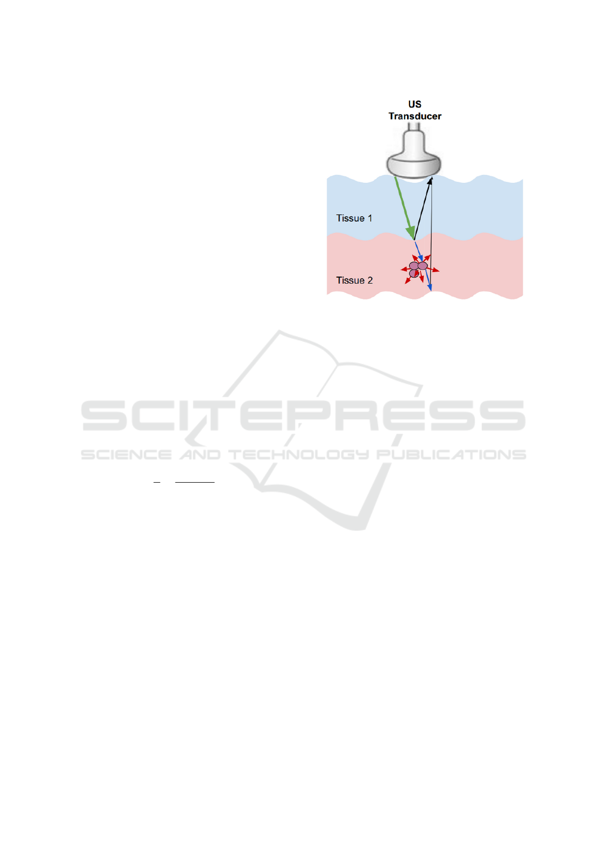
1.2.1 Reﬂection

Reﬂection happens at the boundaries between adja-

cent tissues – the acoustic boundaries. Based on the

size of the boundary relative to the US beam wave-

length, or the irregularities of the surface of the reﬂec-

tor, we can divide the reﬂection into two categories:

the specular reﬂection and the non-specular reﬂec-

tion. Specular reﬂection happens when the bound-

ary is smooth and longer than the beam dimensions,

while non-specular reﬂection occurs when the size of

the reﬂector is smaller than the wavelength of the ul-

trasound beam.

The reﬂection coefﬁcient on the acoustic surface

is given by

− z

)

+ z

)

(2)

where I

is the intensity of the incident beam, I

the intensity of the reﬂected beam, z

is the acoustic

impedance of the ﬁrst medium, and z

is the acoustic

impedance of the second medium.

The more the difference between the impedance

values (acoustic mismatch), the larger the echo.

The irregularity in the shape of the reﬂecting sur-

face or its small dimensions reﬂects the incident beam

in many directions is known as US scattering.

The scattering strongly depends on the US fre-

quency, so it increases as the frequency increases.

ν = f × λ (3)

where ν is the sound velocity, f is the frequency, and

λ is the wavelength. See Figure 1.

1.2.2 Absorption

During absorption, the US energy gets converted into

heat. Three factors affect absorption – the viscosity of

the medium, the relaxation time of the medium, and

Figure 1: Ultrasound interaction with tissues. The green,

black, red, blue arrows represent the incident wave, the

specular reﬂection, the non-specular reﬂection, and the re-

fracted wave, respectively.

the frequency of the beam. Absorption increases in

direct proportion to all three factors. The viscosity is

generated from the frictional forces between the par-

ticles. The relaxation time is the duration required for

the particles of the medium to get back to their mean

position after getting displaced by the US waves. Ab-

sorption also increases with the beam frequency, al-

though increased frequency can enhance details in the

US image.

1.2.3 Attenuation

Attenuation is the reduction of the beam intensity

caused by the total losses throughout the propagation.

Based on the power law (Cong et al., 2013), the en-

ergy attenuation of the ultrasound wave after its prop-

agation in the medium for a distance d is given by:

U(α

re f

, d) = U

× e

−2α

re f

(4)

where α is an attenuation parameter related to the

properties of the propagation medium.

2 RELATED WORK

As we mentioned in the abstract, many researchers

tried to simulate ultrasound images simply by model-

ing US with speckle noise and ignoring other interac-

tions of ultrasound with the tissue.

Goodman modeled speckle noise in laser images

by a Rayleigh distribution (Goodman, 1975). Wagner

et al (Wagner, 1983) represented the speckle noise by

Simulating Ultrasound Images from CT Scans

139

a Rician model. While Shankar (Shankar, 2000) came

up with Nakagami distribution to describe speckle

noise. Usually, Gamma distribution is the best ap-

proximation of speckle noise in SAR images (Ayed

et al., 2005). Zimmer (Zimmer et al., 2000) mod-

eled speckle noise in ultrasound liver images by a log-

normal distribution. Tao et al in (Tao et al., 2006)

proved that Gamma and Weibull distributions are bet-

ter approximations of speckle noise in clinical cardiac

ultrasound images than normal or log-normal distri-

butions.

In (Achim et al., 2001) and (Rabbani et al., 2008),

the authors proposed a method to convert the multi-

plicative noise into an additive noise by logarithmi-

cally transforming the image as follows:

I(x, y) = S(x, y)η(x, y), (5)

where I is the noisy observation (the US image), S is

the noise-free image, and η represents the multiplica-

tive speckle noise.

logI(x, y) = log(S(x, y)) + log(η

(x, y)) (6)

f (x, y) = g(x, y) + ε(x, y) (7)

Shams et al (Shams et al., 2008) proposed a novel

method for simulating ultrasound images from 3D CT

scans. In the proposed method, the authors started

with edge detection of the CT image to calculate the

reﬂection coefﬁcients. Then they generated the scat-

tering image using FieldII (Jensen, 1996) by placing

scatterers with strength randomly chosen by Field II

from a normal distribution. The authors indicated that

using this method to create a realistic speckle pattern

is very computationally expensive. For instance, sim-

ulating a B-mode image with 128 RF scan lines takes

nearly two days.

Kutter et al (Kutter et al., 2009) proposed a

simulation-based registration pipeline of US to CT

images in real-time. They developed a simple ray-

based modeling of ultrasound images using OpenGL

software (Woo et al., 1999). They used a Lambertian

scattering model to simulate the scattered signal. And

they generated a scattering image using Field II soft-

ware. In (Reichl et al., 2009), the US intensity at the

location of the probe was adjusted at ﬁrst. Then, the

amount of intensity transmitted, reﬂected, or absorbed

along each column (each scanline) of the image was

computed for every pixel according to the propagation

characteristics. After that, the reﬂection and the ab-

sorption were subtracted from the incident intensity at

every pixel. Finally, in the post-processing stage, arti-

facts such as speckle noise and blurring were added

to the ultrasound images. In their proposed work,

speckle noise was characterized by a Rayleigh distri-

bution.

Feng Gu et al. proposed a genrative adversarial

network (GAN) to model the speckle noise in syn-

thetic aperture radar (SAR) images (Gu et al., 2019).

In this work, we present a novel method for sim-

ulating the interaction pattern between the ultrasound

waves and the tissue, that is inspired by the underly-

ing physics of ultrasound image generation, starting

from CT images of different body parts.

3 PROPOSED METHOD

Our proposed method for generating ultrasound im-

ages from CT images consists of two stages – generat-

ing speed of sound images from CT images, and gen-

erating US images from speed of sound images. The

code of our proposed method is available at (Nasser

and Sethi, ).

3.1 Generating Speed of Sound Images

from CT Images

To generate the speed of sound images from CT im-

ages, we use the fact that the intensity value of a spe-

ciﬁc pixel of a 2D CT image represents the Hounsﬁeld

unit (HU) of the underlying tissue that corresponds to

that pixel. HU is a measure of X-ray attenuation in

the tissue. Given a tissue x, the HU is given by:

= 1000 ×

− µ

water

(8)

where µ

is the total linear attenuation coefﬁcient of

the tissue x at a given x-ray energy. µ

of a tissue x can

be computed from multiplying the mass density of a

tissue x (ρ

) by the weighted sum of the mass attenu-

ation coefﬁcients of all the elements which compose

the tissue x, as shown in the following equation:

= ρ

∑





(9)

where

is the mass attenuation coefﬁcient of the el-

ement (i) in cm

/g. Table 1 shows the elemental com-

position (w

values) of a few of the body tissues taken

from the ITIS database (ITI, ).

Given the kilovoltage peak applied to the X-ray

tube for capturing CT images is 120 kPv, and w

val-

ues from (ITI, ), we can compute the mass attenuation

coefﬁcient of each element in the elemental composi-

tion of a certain tissue by using NIST software (NIS,

). NIST allows us to compute the mass attenuation

coefﬁcients of the tissues, which, in turn, allows us to

compute their corresponding HUs by substituting the

values in equation 8.

BIOIMAGING 2023 - 10th International Conference on Bioimaging

140

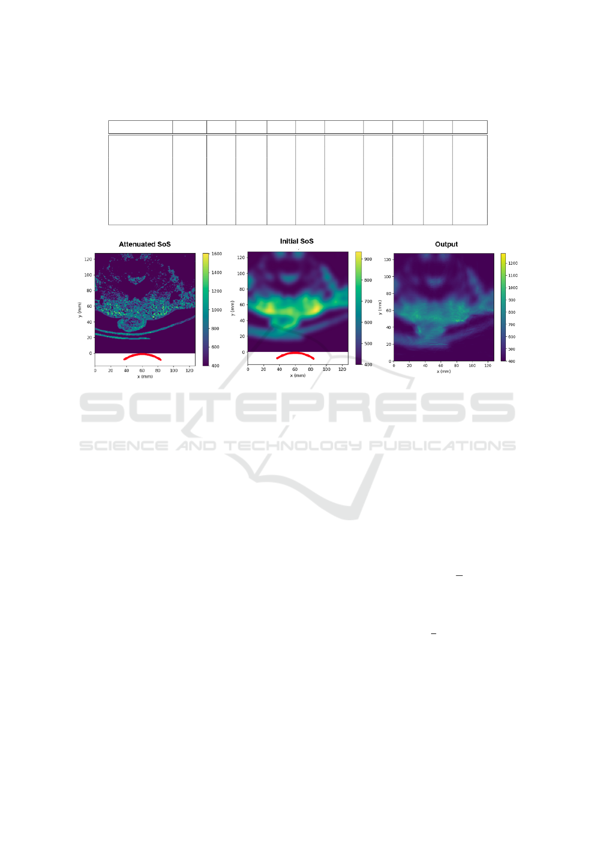
Table 1: Examples of the composition of a few of the body tissues. This table does not include the values of all the elements

of the tissue composition, other elements, such as silicon and phosphorus, can be found in (Ele, ).

Tissue Hydrogen Carbon Nitrogen Oxygen Sodium Magnesium Sulfur Chlorine Argon Potassium

Air 0 0.00015 0.78 0.21 0 0 0 0 0.0047 0

Liver 0.63 0.073 0.013 0.28 0.00054 0 0 0.0006 0.00058 0.00035

Prostate 0.64 0.046 0.011 0.3 0.00054 0.0002 0.00039 0 0 0.00032

Fat 0.5 0.37 0.003 0.13 0.00018 0.0005 0.00013 0.00012 0 0

Kidney 0.63 0.069 0.013 0.28 0.00054 0.0004 0.00039 0.00035 0 0.00032

Urinary Bladder Wall 0.64 0.049 0.011 0.29 0.00054 0.0004 0.00039 0.00052 0 0.00047

Urine 0.66 0.0025 0.0043 0.33 0.0011 0.0002 0 0.001 0 0.00031

Water 0.67 0 0 0.33 0 0 0 0 0 0

Figure 2: The images from left to right are the attenuated speed of sound (SoS) image (the input of the forward pass), the

initial speed of sound image (the input of the backward pass), and the output of Stride software.

Now having the speed of sound values and the cor-

responding HU values of the tissues at 37 Celsius, we

can generate the speed of sound images from the cor-

responding CT images.

We simulate the attenuation of US waves in tissues

using equation (4),

3.2 Generating US Images from Speed

of Sound Images

In the second stage of our proposed method, we sim-

ulate the US images from the speed of the sound

images. For simulating ultrasound images from the

speed of sound images which we generate, we use

Stride software (Cueto et al., 2022). Stride is an

open-source library for ultrasound computed tomog-

raphy. Unlike the methods based on full-waveform

inversion, Stride is not computationally expensive.

Stride is user-friendly software, and the code can be

run on CPUs and GPUs. This tool is based on a

domain-speciﬁc language called Devito which gener-

ates solvers of the wave-equation.

We can summarize the overall workﬂow of this

software to reconstruct the image of the tissue from

the measurements as follows:

1. The sensors produce acoustic waves, which prop-

agate throughout the medium. These propagated

waves get reﬂected on the acoustic boundaries of

the medium.

2. The reﬂected waves get captured by the receivers.

3. The acquired data is used to reconstruct the phys-

ical properties of the medium, for instance, the

speed of the wave through it and its density.

4. The reconstruction procedure minimizes the mis-

ﬁt between the recorded measurements and the

numerically modeled ultrasound data.

Thus from a set of measurements of the pressure

wave ﬁeld u, we can build an accurate model of the

discrete wave velocity C (or m =

) by consider-

ing it as a partial differential equation-constrained op-

timization problem, where the objective function is

given by:

minimize

(m) =

||p

u − d||

(10)

with u = A(m)

−1

, where p

is the sampling op-

erator of receiver locations, P

represents the injec-

tion operator at source locations, A(m) is the discrete

isotropic wave equation matrix, u is the discrete pres-

sure wave ﬁeld, q

is the pressure source, and d is the

measured date.

Simulating Ultrasound Images from CT Scans

141

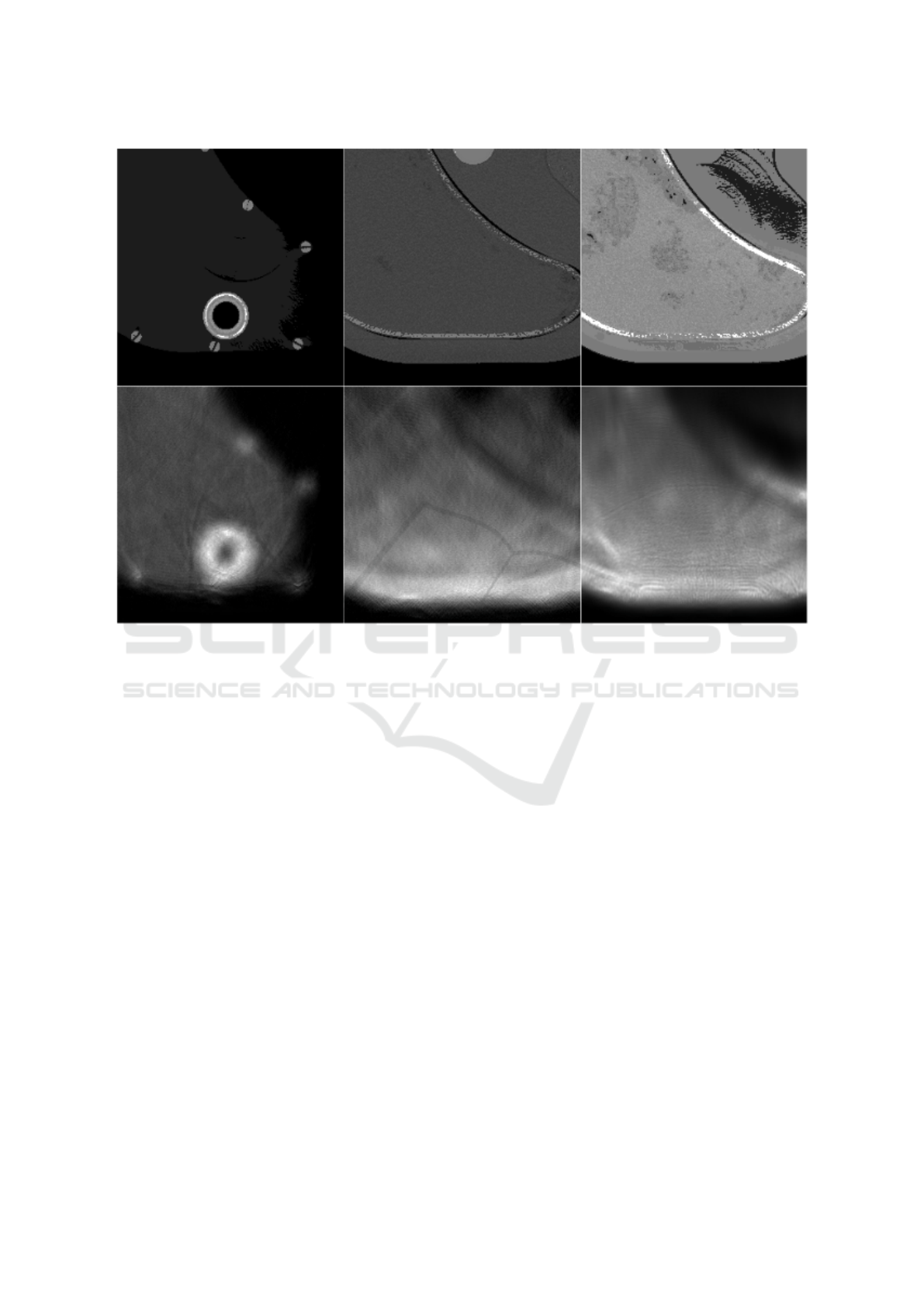
Figure 3: A few example output images of our proposed method for ultrasound simulation. The images are three different

slices of a phantom of the liver. The ﬁrst row contains the speed of sound images generated from the corresponding CT images

(Ima, ). The second row contains the simulated ultrasound images. The experiments from left to right are a simulation using

a linear probe without attenuation, a simulation using a linear probe with attenuation, and a simulation using a curvilinear

probe with attenuation correspondingly.

By solving the optimization problem based on the

gradient method (Plessix, 2006) (Haber et al., 2012)

we get:

∆Φ

(m) = sum

t=1

u[t]ν

[t] = J

δd

(11)

where n

is the number of steps, δd

= p

u − d is the

data residual between the measured and the modeled

data, J is the Jacobian operator, ν

is the second-order

time derivative of the adjoint wave ﬁeld A

(m)ν =

δd

4 RESULTS AND DISCUSSION

We designed a curvilinear transducer similar to the

one used by clinicians for abdominal imaging. The

transducer has a central frequency of 2.5 MHZ, a

number of elements equals 64, a radius of the cur-

vature equals 5R, and a curvature equals 50 mm.

The simulation consists of a forward pass and a

backward pass. For the backward pass, rather than

starting from a ﬁxed speed of sound, we started from

an initial estimation of the speed of the sound image

to improve convergence. This initial estimation is a

blurred version of the ground truth speed of the sound

image. See Figure 2.

Figure 3 shows a few results of our proposed

method for ultrasound simulation. One can see in the

simulated US image the arc artifacts that are found in

real ultrasound images when a curvilinear transducer

is used.

In ﬁgure 4, we try to qualitatively assess our re-

sults by visually comparing the simulated images with

real US images. In ﬁgure 4, the CT images and real

US images were taken from (Ima, ), (AbU, ).

We refer to the work presented in (Kutter et al.,

2009) and (Reichl et al., 2009) for visual comparison

with the results of our proposed method. In our sim-

ulation, we use Stride software built upon the open-

source programming language (Python). While meth-

ods (Kutter et al., 2009) and (Reichl et al., 2009) use a

Matlab-based software called Field II. For a fair com-

parison between our methods and other methods, our

extended paper should incorporate a comparison be-

BIOIMAGING 2023 - 10th International Conference on Bioimaging

142

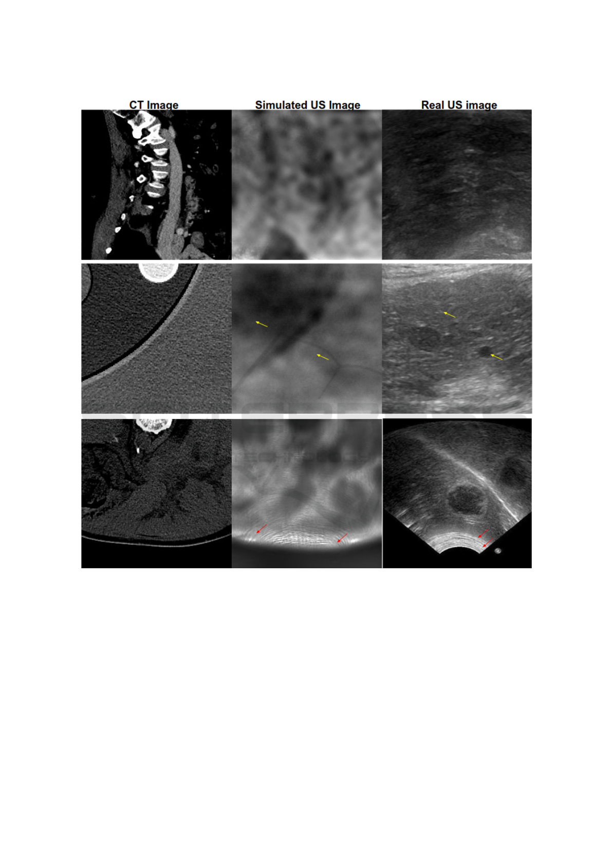
Figure 4: The ﬁrst two columns contain CT images and the corresponding simulated ultrasound images, while the third

column contains real ultrasound images which do not correspond to CT images. The red arrows indicate the arc artifacts in

both real and simulated US images. The yellow arrows indicate the granular texture in simulated and real US images. For a

precise comparison between our simulated images and real US ones, we are planning further experiments in which we acquire

CT scans of a phantom to simulate ultrasound images using our proposed method. After that, we can compare the simulated

US images with the real US images of the same phantom.

tween these methods for the same ground truth CT

images, and the same US imaging probe.

5 CONCLUSIONS

In this work, we showed promising results in sim-

ulating US images from CT images. The wave in-

terference pattern and other artifacts were similar to

real US images. Our proposed method for obtain-

ing the simulated ultrasound images from the CT im-

Simulating Ultrasound Images from CT Scans

143

ages needs further improvement. After optimizing the

hyper-parameters of our simulation we will be able

to form a paired dataset (CT-Ultrasound pairs) which

can be used for training a generative adversarial net-

work GAN in a supervised manner and ﬁnally testing

it on reconstructing the CT images from the real US

images. The potential utility of this work is to train

deep neural networks for the inverse problem of sim-

ulating CT images from the given US images, which

can aid clinicians in diagnosis and surgical interven-

tion.

ACKNOWLEDGEMENT

This work would not have been possible without the

ﬁnancial support of the Qualcomm Innovation Fel-

lowship Award, India. We are indebted to the devel-

oper of Stride, Mr. Carlos Cueto from Imperial Col-

lege London, for his feedback and support.

REFERENCES

Abdominalultrasonography. https://

todaysveterinarypractice.com/radiology-imaging/

imaging-essentialssmall-animal-abdominal-ultrasono

graphy-part-2-physical-principles-artifacts-false-

assumptions/. Accessed: 2021-10-24.

Cancer imaging archive. https://www.

cancerimagingarchive.net/. Accessed: 2021-10-

24.

Computing the mass attenuation coefﬁcients of the ele-

mental composition of the tissues. https://www.nist.

gov/pml/xcom-photon-cross-sections-database. Ac-

cessed: 2021-10-24.

Element composition of the body tissues. https:

//itis.swiss/virtual-population/tissue-properties/

database/elements/. Accessed: 2021-10-24.

ITIS Foundation. https://itis.swiss/virtual-population/

tissue-properties/database/elements/. Accessed:

2021-10-24.

Achim, A., Bezerianos, A., and Tsakalides, P. (2001).

Novel bayesian multiscale method for speckle re-

moval in medical ultrasound images. IEEE transac-

tions on medical imaging, 20(8):772–783.

Ayed, I. B., Mitiche, A., and Belhadj, Z. (2005). Multire-

gion level-set partitioning of synthetic aperture radar

images. IEEE Transactions on Pattern Analysis and

Machine Intelligence, 27(5):793–800.

Cong, W., Yang, J., Liu, Y., and Wang, Y. (2013). Fast

and automatic ultrasound simulation from ct im-

ages. Computational and mathematical methods in

medicine, 2013.

Cueto, C., Bates, O., Strong, G., Cudeiro, J., Luporini, F.,

Agudo,

O. C., Gorman, G., Guasch, L., and Tang, M.-

X. (2022). Stride: A ﬂexible software platform for

high-performance ultrasound computed tomography.

Computer Methods and Programs in Biomedicine,

221:106855.

Duarte-Salazar, C. A., Castro-Ospina, A. E., Becerra,

M. A., and Delgado-Trejos, E. (2020). Speckle noise

reduction in ultrasound images for improving the

metrological evaluation of biomedical applications:

an overview. IEEE Access, 8:15983–15999.

Goodman, J. W. (1975). Statistical properties of laser

speckle patterns. In Laser speckle and related phe-

nomena, pages 9–75. Springer.

Gu, F., Zhang, H., and Wang, C. (2019). A gan-based

method for sar image despeckling. In 2019 SAR in

Big Data Era (BIGSARDATA), pages 1–5. IEEE.

Haber, E., Chung, M., and Herrmann, F. (2012). An effec-

tive method for parameter estimation with pde con-

straints with multiple right-hand sides. SIAM Journal

on Optimization, 22(3):739–757.

Jensen, J. A. (1996). Field: A program for simulating ultra-

sound systems. In 10TH NORDICBALTIC CONFER-

ENCE ON BIOMEDICAL IMAGING, VOL. 4, SUP-

PLEMENT 1, PART 1: 351–353. Citeseer.

Kaplan, D. and Ma, Q. (1994). On the statistical character-

istics of log-compressed rayleigh signals: Theoretical

formulation and experimental results. The Journal of

the Acoustical Society of America, 95(3):1396–1400.

Kutter, O., Shams, R., and Navab, N. (2009). Visualization

and gpu-accelerated simulation of medical ultrasound

from ct images. Computer methods and programs in

biomedicine, 94(3):250–266.

Mather, P. and Tso, B. (2016). Classiﬁcation methods for

remotely sensed data. CRC press.

Nasser, S. A. and Sethi, A. Simulat-

ing Ultrasound Images From Ct Scans.

https://github.com/SaharAlmahfouzNasser/Simulating-

Ultrasound-images-from-CT-Scans.git.

Plessix, R.-E. (2006). A review of the adjoint-state method

for computing the gradient of a functional with geo-

physical applications. Geophysical Journal Interna-

tional, 167(2):495–503.

Rabbani, H., Vafadust, M., Abolmaesumi, P., and Gazor, S.

(2008). Speckle noise reduction of medical ultrasound

images in complex wavelet domain using mixture pri-

ors. IEEE transactions on biomedical engineering,

55(9):2152–2160.

Reichl, T., Passenger, J., Acosta, O., and Salvado, O.

(2009). Ultrasound goes gpu: real-time simulation

using cuda. In Medical Imaging 2009: Visualiza-

tion, Image-Guided Procedures, and Modeling, vol-

ume 7261, pages 386–395. SPIE.

Shams, R., Hartley, R., and Navab, N. (2008). Real-time

simulation of medical ultrasound from ct images. In

International Conference on Medical Image Comput-

ing and Computer-Assisted Intervention, pages 734–

741. Springer.

Shankar, P. M. (2000). A general statistical model for ultra-

sonic backscattering from tissues. IEEE transactions

on ultrasonics, ferroelectrics, and frequency control,

47(3):727–736.

BIOIMAGING 2023 - 10th International Conference on Bioimaging

144

Singh, P., Mukundan, R., and de Ryke, R. (2017). Synthetic

models of ultrasound image formation for speckle

noise simulation and analysis. In 2017 International

Conference on Signals and Systems (ICSigSys), pages

278–284. IEEE.

Tao, Z., Tagare, H. D., and Beaty, J. D. (2006). Evaluation

of four probability distribution models for speckle in

clinical cardiac ultrasound images. IEEE transactions

on medical imaging, 25(11):1483–1491.

Tole, N. M. et al. (2005). Basic physics of ultrasonographic

imaging. World Health Organization.

Wagner, R. F. (1983). Statistics of speckle in ultrasound

b-scans. IEEE Trans. Sonics & Ultrason., 30(3):156–

163.

Woo, M., Neider, J., Davis, T., and Shreiner,

D. (1999). OpenGLprogramming-

guide:theofﬁcialguidetolearningOpenGL,version1.2.

Addison-WesleyLongmanPublishingCo.,Inc.

Zimmer, Y., Tepper, R., and Akselrod, S. (2000). A lognor-

mal approximation for the gray level statistics in ul-

trasound images. In Proceedings of the 22nd Annual

International Conference of the IEEE Engineering in

Medicine and Biology Society (Cat. No. 00CH37143),

volume 4, pages 2656–2661. IEEE.

Simulating Ultrasound Images from CT Scans

145