An Artificial Dendritic Neuron Model Using Radial Basis Functions
Zachary Hutchinson
a
University of Maine, SCIS, Orono ME 04469, U.S.A.
Keywords:
Artificial Dendrites, Neural Model, Neural Computation.
Abstract:
The dendrites of biological neurons are computationally active. They contribute to the expressivity of the
neural response. Thus far, dendrites have not seen wide use by the AI community. We propose a dendritic
neuron model based on the compartmentalization of non-isopotential dendrites using radial basis functions.
We show it is capable of producing Boolean behavior. Our goal is to grow the AI conversation around more
complex neuron models.
1 INTRODUCTION
1.1 Neural Communication
Neurons send and receive information through differ-
ent parts of the cell. Generally, output leaves the neu-
ron via the axon and enters through the dendrite. Both
axon and dendrite extend from the cell body; however,
dendrites typically take on far more elaborate shapes.
A single neuron can have many distinct dendrites em-
anating from different sides of the cell body. Den-
drites can have hundreds of branches and form con-
nections with tens- to hundreds of thousands of other
neurons (Fox and Barnard, 1957; Megıas et al., 2001).
The dendrite is the computational workhorse of
the biological neuron; they are not merely wires by
which neurons reach distant sources. The dendrite
performs active and passive computational duties by
transforming, filtering and integrating signals within
the dendritic tree before they reach the soma. This
innate ability to transform incoming signals enhances
the overall computational power of the neuron (Cuntz
et al., 2014). The computational enhancement of the
biological neuron by its own input structure was de-
scribed succinctly by Papoutsi et al:
[...] compartmentalization of information pro-
cessing endows neurons with a second pro-
cessing layer that boosts the computational ca-
pacity of the neuron by at least an order of
magnitude compared to that of a thresholding
point neuron.(Papoutsi et al., 2014)
a
https://orcid.org/0000-0001-7584-0803
Although neuroscience has produced decades of
research into the rich computational nature of the bi-
ological dendrite, it has been largely ignored by the
artificial intelligence community. This case of the
missing dendrite dates all the back to the original
neuroscience-to-AI translation made by McCulloch
and Pitts:
The nervous system is a net of neurons, each
having a soma and an axon. Their adjunc-
tions, or synapses, are always between the
axon of one neuron and the soma of an-
other.(McCulloch and Pitts, 1943)
1.2 Motivation and Related Work
The motivation for this paper is to propose a simple
dendritic neuron model for use in AI tasks. In propos-
ing a basic dendritic model we hope to spur interest
in more complex neuron models within the artificial
neural network (ANN) community. AI-related den-
dritic research is in its infancy. We take our cues from
neuroscience research which suggests that dendritic
transformation of neural signals is important to neu-
ral computation. The benefits of this transformation
with respect to current AI standards and techniques is
an open question.
Several recent AI works have experimented with
more complex neuron models. These have been cre-
ated using multiple sigmoidal functions along den-
dritic branches (Teng and Todo, 2019), additional
sub-layers of point neurons (Jones and Kording, 2020;
Wu et al., 2018) and in hardware (Elias, 1992; Elias
et al., 1992). The majority of related work focuses
on demonstrating results with different benchmark
776
Hutchinson, Z.
An Artificial Dendritic Neuron Model Using Radial Basis Functions.
DOI: 10.5220/0011775400003393
In Proceedings of the 15th International Conference on Agents and Artificial Intelligence (ICAART 2023) - Volume 3, pages 776-783
ISBN: 978-989-758-623-1; ISSN: 2184-433X
Copyright
c
 2023 by SCITEPRESS – Science and Technology Publications, Lda. Under CC license (CC BY-NC-ND 4.0)

data sets. Accuracy of classification says little about
the nature of the computational benefits of dendrites.
Therefore, we hope to balance this with a simple
model which captures several key aspects of non-
isopotential dendrites.
Computational neuroscience has produced a
plethora of neuron models which include dendrites,
starting with those based on cable theory in the 1960s
(Rall, 1964). Neuroscientific neuron models are de-
signed to mimic the real thing and therefore con-
tain mathematical approximations of ion channels,
membrane capacitance and resistance, distributions
of synapses, dendritic spikes and other biophysical
attributes. Properties are added or removed based
on which neuron and dendritic characteristic is be-
ing studied (Bower, 2015; Mel, 2016; Poirazi and
Papoutsi, 2020). Their construction is guided by the
morphology of a specific neuron type. While model
elements might be amenable to AI uses, the hand-
crafted approach to morphology is not.
2 MODEL
The artificial dendritic neuron model (AD neu-
ron) highlights two biophysical aspects of the den-
drite: compartmentalization and separation. Den-
drites are non-isopotential entities; this ability to
maintain varying electrical potentials across its length
and branches is thought to divide the dendritic tree
into compartments. Each compartment is a quasi-
independent computational unit. Within each com-
partment, synaptic inputs interact more immediately
and linearly; whereas, between compartments signals
are subject to delays and nonlinear transformations
(Beniaguev et al., 2021; Polsky et al., 2004; H
¨
ausser
and Mel, 2003). The character of the nonlinear trans-
formation depends on dendritic properties between
two sites. These intervening properties we generalize
into the concept of separation between compartments.
The AD neuron model is comprised of two fun-
damental elements: compartments and connections.
Compartments receive and evaluate input from other
compartments. And connections specify an input-
output relationship over all compartments.
2.1 Compartment
The dendritic neuron model is a tree-like structure
comprised of compartments. Each compartment com-
putes the combination (e.g. sum) of the input vector,
I.
Definition: A compartment is by its output func-
tion:
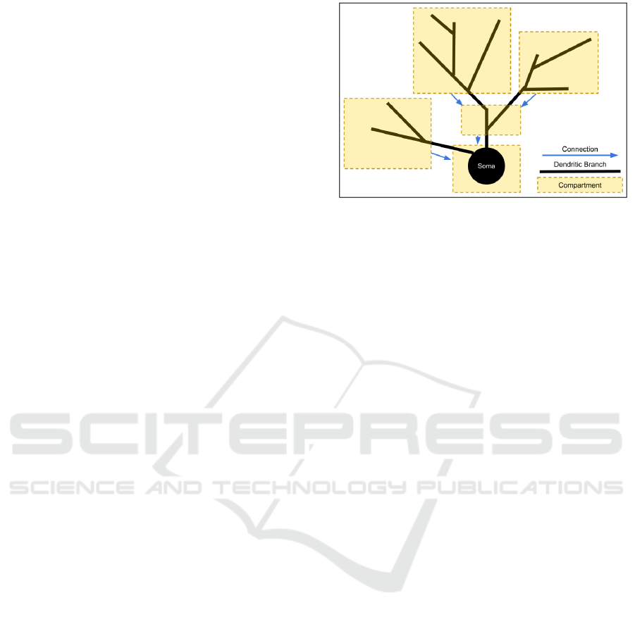
Figure 1: Compartmentalization of the dendritic neuron.
A dendritic neuron (black) is broken into several compart-
ments (dotted yellow). The underlying shape of the den-
dritic tree is used to create matching connections (blue ar-
rows) between compartments.
v
a
= ψ(z),where z =
n
∑
i=0
x
i
(1)
v
a
gives the output of a dendritic compartment. I
is the input vector [v
1
,v
2
,...,v
n
]
T
. ψ is an activation
function. ψ is not strictly defined by the basic AD
neuron model because it is a placeholder for any acti-
vation function.
By this definition, the dendritic neuron compart-
ment is identical to a basic perceptron or point neu-
ron which outputs the sum of its inputs modified by
a nonlinear activation function. There is one clear
distinction between the perceptron and the dendritic
compartment. A perceptron describes a whole neu-
ron; whereas, a compartment is capable of describing
the whole neuron or just a part of it. The effect of this
is: whereas a perceptron receives all inputs to its den-
dritic field, a dendritic compartment can receive just
a subset of the inputs. Additionally, ψ is allowed to
vary between compartments within the same neuron.
Figure 1 shows how compartments form an ab-
straction of a dendritic tree by grouping branches into
separate entities. Because compartments represent
swaths of the dendritic tree, they can encapsulate the
location of one or more inputs to the AD neuron.
Compartments, or the compartmentalization of a
dendritic tree, respect three rules:
No-skip Rule: If a compartment, C, contains two
input locations, i and j, then there does not exist a k
between i and j along the dendritic branch such that
k /∈ C. In other words, compartments cannot skip over
input locations. An addendum to this rule is that if
two inputs share the same tree location, they are also
in the same compartment.
Order Rule: If a compartment, C, contains two
input locations, i and j, and the distances between
them and the soma is d
i
and d
j
such that d
i
> d
j
, then
An Artificial Dendritic Neuron Model Using Radial Basis Functions
777

ˆ
d
i
≥
ˆ
d
j
, where
ˆ
d is their distance-to-soma after com-
partmentalization. Or to put it another way, compart-
mentalization is order preserving. The compartmen-
talized tree forms a non-strict partial order of the AD
neuron’s inputs.
Intersection Rule: Let i and j be two inputs to the
AD neuron located on different dendritic branches. If
a compartment, C, contains the two input locations, i
and j, such that i, j ∈ I
C
, the input vector to C, then
I
C
must contain all inputs on the dendrite between i
and j. To find all inputs between i and j we follow
the dendrite from one to the other. All inputs encoun-
tered must be in C. This prevents a compartment from
including multiple branches of the dendritic tree with-
out also including the intersection of those branches.
This rule is an elaboration on the No-skip Rule.
2.2 Connection
Definition: A connection is defined by a 4-tuple
(c
i
,c
j
,v
e
,ϕ).
c
i
and c
j
are dendritic compartments which define
the start and end of a connection. c
i
is the compart-
ment whose output is input to the connection and c
j
is
the compartment which receives the output of the con-
nection. From this, we say that c
i
is adjacent to c
j
. ϕ
is a radial basis-like function which defines the effect
the connection has on a signal passing from compart-
ments c
i
to c
j
. v
e
is a value in R that measures the
separation between the compartments and is used by
ϕ as the center from which metric of the radial basis
evaluates input.
3 THE EXPANDED MODEL
The expanded dendritic model diversifies the ba-
sic model to constrain compartmental connectivity
around a biological model and to more precisely de-
fine the role of ϕ.
3.1 ϕ
The base model simply defines ϕ as a radial basis-
type function (RBF) which makes use of a center or
expected value, v
e
. We can expand the four-tuple of
the base model to include two more parameters. b
and w, which allow connections to adjust the shape
and amplitude of ϕ’s profile. Equation 2 gives the
expanded version of the AD connection.
ϕ(v
a
) =
w
((v
a
− v
e
)b)
2
+ 1
(2)
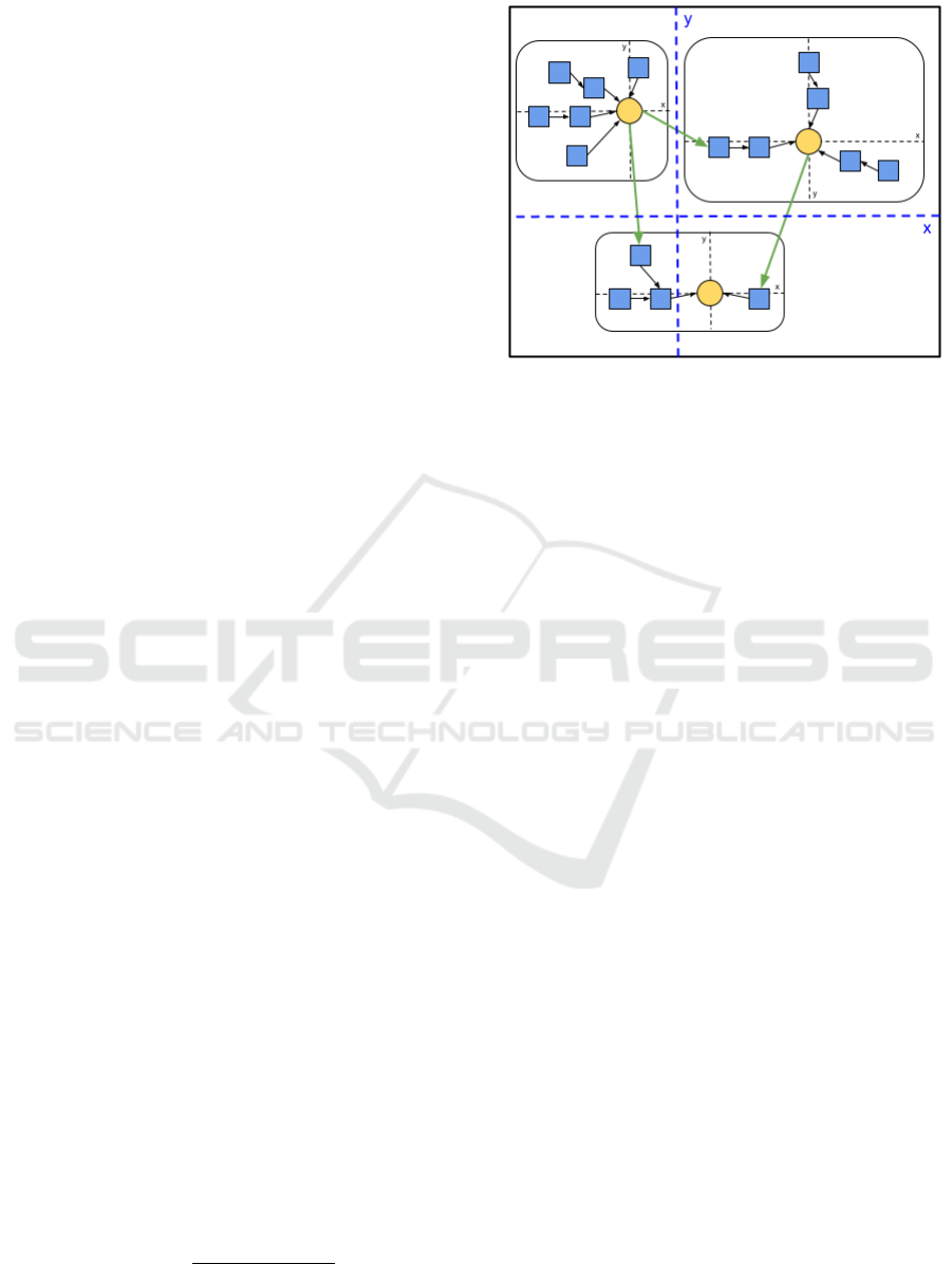
Figure 2: An example of the use of multiple spaces within
a hyperspace. Compartments are placed within spaces
defined by Cartesian x,y-coordinates. Blue squares are
branch compartments and yellow circles are somatic com-
partments. Each soma compartment exists at the origin
within a separate neuronal space and associated, child com-
partments derive their local space values for d with respect
to a local origin. At the same time, each compartment main-
tains a position within the hyperspace coordinate system
(blue axes). In this example, black arrows denote connec-
tions whose values of d rely on the local space. And green
arrows use hyperspace coordinates.
v
a
and v
e
are, as previously stated, the actual and
expected values. v
a
is the output of compartment c
i
(Equation 1). w is the connection’s weight. And b
is a shape parameter which determines the range over
which activation occurs. Again, each connection has
its own w, v
e
and b. These are connection-level pa-
rameters. They belong to the connection because con-
nections, during a training process, might swap termi-
nal compartments.
3.2 Two Concerns: Relevance and
Importance
Why do connections use an RBF to transform the sig-
nals passing from one compartment to another?
An RBF allows the dendritic neuron model to sep-
arate two concerns which in the point neuron model
are somewhat conflated. These concerns are the rel-
evance of a specific value to the receiving compart-
ment and the importance of the connection carrying
the signal.
Relevance is the meaning assigned by the con-
nection to a specific value of v
a
. The magnitude of
a signal is not its relevance. Connections are like a
combination lock. The more v
a
matches v
e
, the more
a connection opens. The closer it is, the more relevant
it is. The shape parameter b helps to define the range
of relevant signals (i.e. the range of activation).
ICAART 2023 - 15th International Conference on Agents and Artificial Intelligence
778

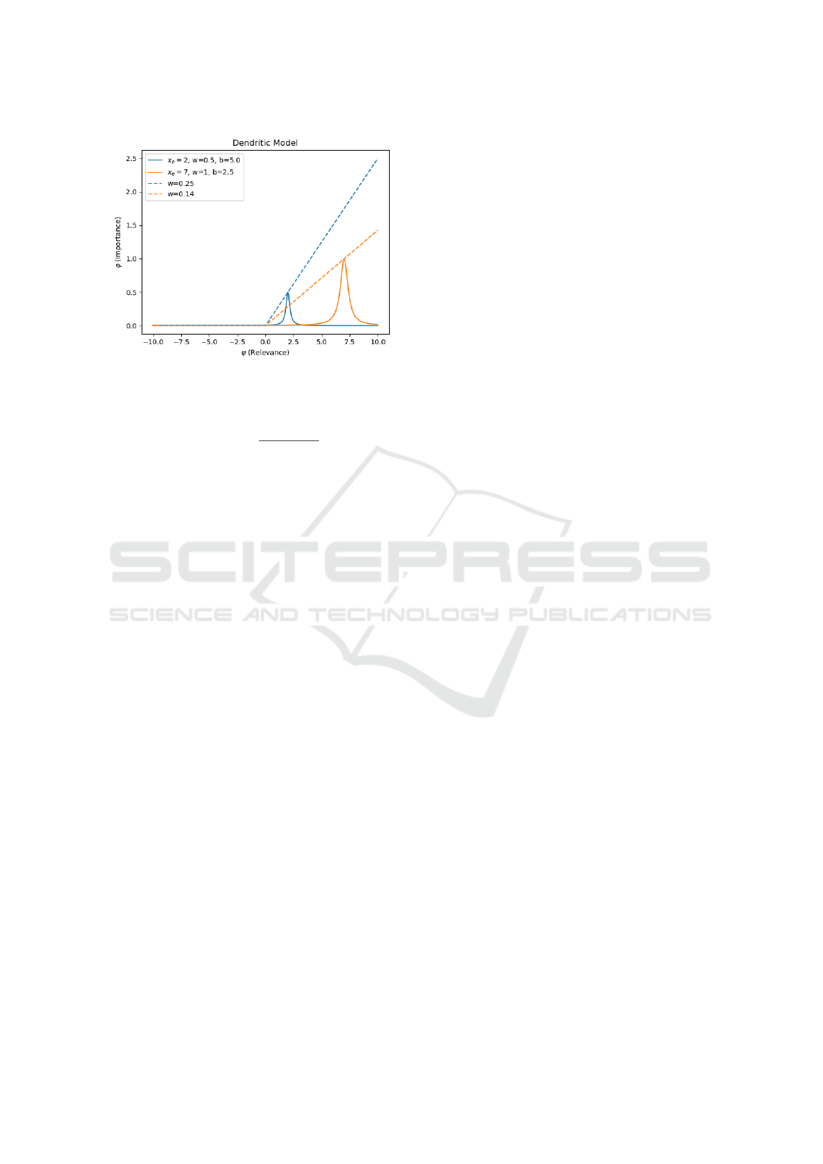
Figure 3: Comparison of how one output signal (ψ) is re-
ceived by two neuron models. Both models receive output
from an assumed ψ which in this case is an ReLU function.
Solid lines show how dendritic connections transform their
input and dashed lines show how point neurons do it. For
dendritic connections ϕ(v
a
) =
w
((v
a
−v
e
)b)
2
+1
. For the point
neuron ϕ(v
a
) = v
a
w. The weights of the point neuron were
chosen so that for the same input both versions of ϕ will
output the same value for v
a
= 2 and v
a
= 7 respectively.
Importance is the strength of a connection with
respect to its sibling connections. Sibling connec-
tions are defined as all connections with the same c
j
,
or end compartment. Importance is controlled by w.
Weight ranks sibling connections with respect to A)
each other and B) the generation of compartmental
output. For example, if w is relatively small, no mat-
ter how close v
a
is to v
e
, its impact on ψ’s output will
be small. Inversely, relatively large w allow one con-
nection to dictate the output of an entire compartment.
In the point neuron relevance is the magnitude of
a signal. The only way for a connection to reduce
the relevance of a signal is to minimize its weight. In
other words, it is impossible for a point to neuron to
make a weak signal relevant without also making a
strong signal even more relevant, and vice versa.
The expanded model was designed to allow for a
greater control over these two concerns.
Figure 3 shows the differences between a point
neuron’s and the AD neuron’s ability to assign mean-
ing to input. Input values (ϕ) over two dendritic (solid
lines) and point neuron (dashed lines) connections are
shown. The dendritic connection in blue has a lesser
importance, i.e. weight, (0.5) compared to the orange
(1.0). The point neuron weights were chosen such that
for the value of ψ at the peak dendritic input, ϕ pro-
duces an identical value for both types. To match the
weaker (less important) dendritic compartment con-
nection (solid blue) requires a stronger weight in the
corresponding point neuron (dashed blue) compared
to the other (dashed orange). In other words, the roles
are reversed; the signal received by the blue point neu-
ron has a greater absolute importance than the orange.
The point neuron treats smaller inputs as less impor-
tant and, therefore, must increase the weight to endow
greater importance at lower values.
In this example, for the point neuron model, the
magnitude of a value is its relevance. This is due to
the binary use of the neural signal: less magnitude,
less relevant; and vice versa. The only way for a
point neuron model to diminish relevance of a signal
is to diminish the importance (weight) of a connec-
tion. The dendritic model, on the other hand, disasso-
ciates a signal’s relevance from its value through the
use of input-side RBFs. Each downstream compart-
ment can assign a different meaning to the same sig-
nal. The disassociation of value and relevance frees
a connection’s weight from the dual responsibility of
determining relevance and importance.
3.3 The Benefits of Separation
Relevance and importance are a product of modeling
the separation of network components and the den-
dritic model is based on the idea that separation itself
possesses computational significance. What compu-
tational characteristics do these products of separation
bring to the dendritic neuron? The separation of rel-
evance and importance has three primary, intertwined
computational effects: democracy of signals, connec-
tion determines meaning, and computation through
coincidence.
The democracy of signals refers to the idea that the
magnitude of a value of a signal is irrelevant to its im-
pact on the receiving compartment. A very small (or
even negative) value can drive the output of a com-
partment just as well as a very large one. The democ-
racy of signals is a direct consequence of divorcing
the relevance of a signal from its importance.
Second, connection determines meaning is the
idea that the meaning of a signal is something locally
determined by each receiving neuron. Both biologi-
cal and artificial neuronal connectivity follows a one-
to-many pattern. Rather than subject every receiving
neuron to the strength of a signal, the AD neuron al-
lows each receiver to determine the meaning of a par-
ticular signal by manipulating v
e
of the intervening
connection.
Third, computation through coincidence refers to
neuronal behavior which is the product of coinciding
activity (or coactivity) at a select set of inputs. Since
dendritic model input signals are evaluated individu-
ally based on their relevance and collectively based
on their importance, the output of a dendritic neuron
depends on the right set of coactive inputs.
An Artificial Dendritic Neuron Model Using Radial Basis Functions
779

3.4 Connectivity
The AD model compartment, by itself, does not make
a dendritic neuron. Alone it is a point neuron. So, to
fully realize the AD neuron model, we must define a
set of rules governing compartmental connectivity.
Let K be the set of compartments which comprise
the dendritic neuron. K can be divided into two dis-
joint sets, S and B, such that:
K = S ∪ B and S ∩ B =
/
0 (3)
|S| = 1 and |B| = |K| − 1 (4)
B contains all branch compartments and S con-
tains all soma compartments. Each compartment’s set
of connections can similarly be partitioned into two
sets, A and E, or the afferent (incoming) and effer-
ent (outgoing) connections. Each of these sets can be
further partitioned into those either coming from or
going to branch or soma compartments. In total, each
compartment’s connections are partitioned into four
sets: A
S
, A
B
, E
S
, and E
B
. For example, the set, A
S
con-
tains all afferent connections from S-compartments.
Partitioning the connections in this way allows us to
create a collection of restrictions on each set. To-
gether, these restrictions define the possible shapes of
a dendritic tree.
Definition: Soma, or S-compartments, are de-
fined by the following restrictions (or lack thereof) on
A and E:
A
S
= {m|m ∈ S and |A
S
| ∈ B
0
}
A
B
= {n|n ∈ B and |A
B
| ∈ B
0
}
E
S
= {m|m ∈ S and |E
S
| ∈ B
0
}
E
B
= {n|n ∈ B and |E
B
| ∈ B
0
}
(5)
Equations 5 place no restrictions soma compart-
ments. They can make afferent and efferent connec-
tions to zero or more soma and branch compartments.
Placing no restrictions on S-compartments is impor-
tant because it allows AD neurons to create both den-
dritic and adendritic subnetworks within a network.
1
Definition: Branch, or B-compartments are de-
fined by the following restrictions on A and E:
A
S
= {m|m ∈ S and |A
S
| ∈ B
0
}
A
B
= {n|n ∈ B and |A
B
| ∈ B
0
}
E
S
= {m|m ∈ S and |E
S
| + |E
B
| = 1}
E
B
= {n|n ∈ B and |E
S
| + |E
B
| = 1}
(6)
1
The existence of adendritic neurons in the brain sug-
gests not all neural computation is best served by dendritic
neurons.
Equations 6 restrict branch compartments such
that they, like the soma compartment, can make un-
restricted afferent connections. They differ from the
S-compartment’s in that they only send output to one
and only one compartment. The type of the efferent
connection is unrestricted
Definition: A dendritic path is defined as the
B-compartments and connections linking two S-
compartments. A path, P, is a dendritic path
if P = {p
0
, p
1
, p
2
,..., p
k
} where p
0
and p
k
are
S-compartments and p
i
,i ∈ {1,k − 1}, are B-
compartments. P is also defined by a set of connec-
tions, P
C
= {c
k,k−1
,c
k−1,k−2
,...c
1,0
}. All dendritic
paths are directed such that there is a connection from
p
i+1
to p
i
.
2
To guarantee the dendritic neuron’s shape
is tree-like, we place a further restriction on dendritic
paths. Given the above definition of a path, we add
that in a dendritic path P, @ i, j | p
i
= p
j
. In other
words, there are no cycles. As a last step, p
k
can
be removed from P. p
k
is removed because it is
the S-compartment, or soma, for an upstream neu-
ron. It was included initially to ensure that the last
B-compartment receives input from at least one S-
compartment.
Two dendritic paths, P and Q, are different if there
exists a p
i
∈ P and a q
i
∈ Q such that p
i
6= q
i
or if
there exists a connection b
i+1,i
∈ P
C
and a connection
c
i+1,i
∈ Q
C
such that b
i+1,i
6= c
i+1,i
. Connections are
equal if their 4-tuples (or 6-tuples in the case of the
extended model) are equal. In other words, two paths
are the same if their compartments and connections
are identical and in the same order.
Definition: A dendritic tree is defined as a
set of dendritic paths terminating in the same S-
compartment which also share at least one B-
compartment. Given an S-compartment, m, a den-
dritic tree of m is a set of dendritic paths D such that
for all P ∈ D, p
0
= m and there exists an n such that
the sub-path {p
0
,..., p
n
} is equivalent (by the above
definition of path difference) for all paths in D.
Definition: A dendritic neuron is defined as a sin-
gle S-compartment and all of its dendritic trees.
The AD neuron model can accommodate any
number of biologically plausible and implausible
morphologies. The following constraints are not
a hard requirement. Generally, we propose these
rules to provide an example how functionally identi-
cal compartments can create complex dendritic trees
through compartment sub-typing.
2
It might seem odd that we are defining direction flow-
ing from p
k
to p
0
rather than the reverse. The choice is
arbitrary in general, but defining it this way simplifies the
definition of dendritic trees which relies on the path defini-
tion.
ICAART 2023 - 15th International Conference on Agents and Artificial Intelligence
780

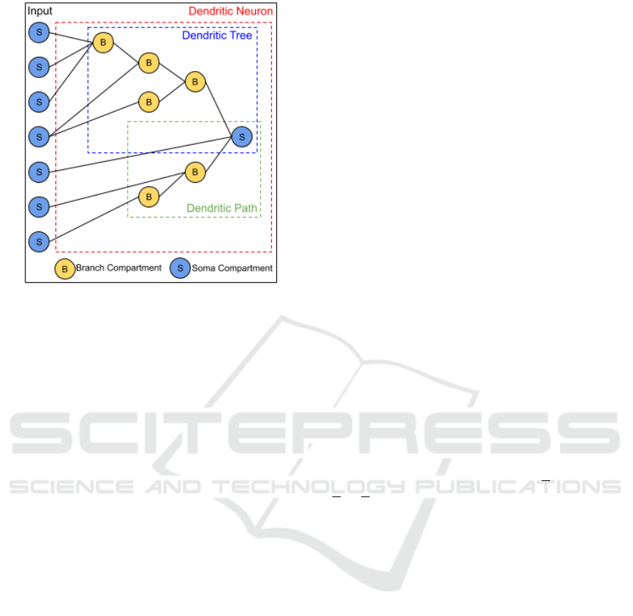
Figure 4: Example of an AD neuron. Black lines are con-
nections.
Figure 4 gives an example of AD neuron connec-
tivity and components. S-compartments can send out-
put to either B- or S-compartments (or both) and they
can send multiple connections to the same AD neuron
(4
th
input). Dendritic paths vary in length; therefore,
inputs receive varying degrees of dendritic process-
ing. The example dendritic path (green box) is also a
dendritic tree because it itself has no branches.
4 COMBINATORICS OF THE AD
NEURON
The number of combinatorial arrangements of the
AD neuron over the point neuron suggests increased
behavioral, and therefore computational, definition.
a(N) gives the number of arrangements of the AD
neuron with N inputs; a(N) is approximated by:
a(N) =
B
|N|
∑
i=1
T (|p
i
|) (7)
where p
i
is the i
th
partitioning of the set of N inputs.
T (n) gives the number of trees possible with n labeled
nodes which is given by Cayley’s formula. B
n
is the
number of partitions of n inputs and is given by the
Bell numbers.
5 BOOLEAN BEHAVIORS
The AD neuron is capable of behaviors which resem-
ble the basic Boolean functions of OR, AND, XOR,
NOR, NAND and IMPLIES. Two of the functions
NAND and OR (bottom row) use two compartments.
IMPLIES uses three. Figure 5 shows how the AD
neuron compartments are configured to produced the
behaviors shown in Figure 6. Both ϕ and ψ utilize
the inverse quadratic RBF (Eq. 2). For all examples,
b = 2 and w = 1 for both ϕ and ψ. All examples re-
ceive input from the same sources, A and B, and pass
through identical versions of ϕ where x
e
= 0.
Boolean behaviors of the AD neuron have several
distinguishing characteristics due to the radial basis
nature of ϕ and ψ. First, the transition from low to
high (or false to true) is fuzzy. The fuzziness and
width of each low/high regions can be adjusted using
larger or smaller values for b. Next, true and false for
some functions is not equal across all regions of truth
and falsehood. For example, OR is true when one
or both inputs are true; however, the AD neuron pro-
duces a higher value when both inputs are true than
when only one is. This can also be seen in AND: pale
blue regions along both x- and y-axes versus the dark
blue as both inputs move away from them.
Complex Boolean behavior can be created by
chaining these elementary examples together. Dia-
gram F in Figure 5 shows how to construct logical
implication, A → B. The bottom center image shows
the results of this construction. Output is false only
when A is true (or A = 0) and B is false (or, B 6= 0).
Again, certain values for A and B produce different
levels of truth. The AD neuron’s version of impli-
cation produces a higher output for A → B than for
A → B.
The AD neuron does face limitations in creating
Boolean functions. Functions such as OR are best
approximated by a threshold; whereas, the AD neu-
ron is best when approximating functions which are
true for unique combinations of input values, such
as XOR, NOR or AND. For example, XOR is true
when the sum of its inputs is one. For NOR, it is zero.
For AND, it is two. More compartments are required
when approximating functions which are true for a
range of values, such as OR, which is true when the
sum of its inputs are one or two. This limitation can
be overcome through the negation of one of the other
functions.
Since the AD neuron is capable of computing, al-
beit fuzzily, Boolean functions, we put forward that
the AD neuron with enough compartments is capa-
ble of computing any logical expression. Additional
experimentation in this area suggests that with more
complexity comes more gray areas with respect truth.
This can be seen in the output of implication (F)
where the regions over which OR is true leave an im-
print on the final result. For very deep dendrites, ear-
An Artificial Dendritic Neuron Model Using Radial Basis Functions
781

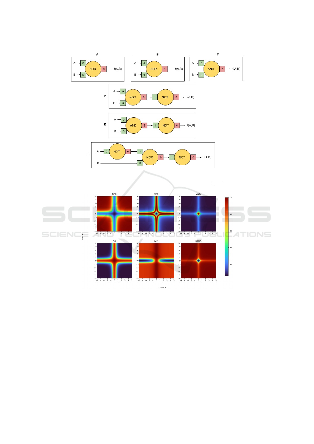
Figure 5: Boolean behaviors: architecture. Yellow circles are AD neuron compartments. Green squares represent the com-
partment’s ϕ function with the numeric value giving x
e
. Red squares represent ψ (an RBF identical to ϕ) with the value giving
its x
e
. (A) Nor (B) Xor (C) And (D) Or (E) Nand (F) Implication, which is implemented as A ∨ B.
Figure 6: Boolean behaviors. The behaviors depicted by these images use the architectures in Figure 5. To create these
images, a sweep was performed over inputs A and B in the range of [-5,5].
lier results can be ‘washed out’ by later ones. There-
fore, constructing very complex Boolean functions
may be challenging and require fine-tuning values for
b, w and x
e
.
6 CONCLUSION
In this paper, we presented both a basic and ex-
tended AD neuron model. The AD neuron consists
of multiple compartments which model the quasi-
independent computational branches of the biological
dendrite. Separation between compartments is mod-
eled using radial basis-type functions. A connectivity
scheme using branch and somatic compartments was
proposed as a structure for creating tree-like dendritic
neurons. Finally, we showed that the AD neuron is
capable of producing Boolean-like behavior.
The central disadvantage of artificial dendrites in
general stems from an increase in model complex-
ity. Dendrites require multiple integrative steps which
must be processed in order. Network topology be-
comes dynamic at a micro level which disrupts par-
ICAART 2023 - 15th International Conference on Agents and Artificial Intelligence
782

allelization and other training optimizations. Weight
modification must take into account the impact of the
dendritic tree on learning signals. Our trainable im-
plementation of the AD uses an RBF metric based
on spike propagation time. We are uncertain how
well compartmental separation can be applied to rate-
based models. The model has not been tested using a
large number of inputs (¿ 100) or in networks with
hidden layers of AD neurons.
There are many open questions related to dendritic
computation. The AI community is faced with a size
and energy bottleneck on the networks we can create.
We need tools allowing us to do more with less which
might require a return to basics and biology. For
the neuroscientific community, there remains a gap in
our understanding how micro-level phenomena con-
struct meso-level information processing which then
contribute to macro-level behaviors. We suspect that
utilitarian neuron models of increased complexity can
make a contribution to both.
REFERENCES
Beniaguev, D., Segev, I., and London, M. (2021). Sin-
gle cortical neurons as deep artificial neural networks.
Neuron, 109(17):2727–2739.
Bower, J. M. (2015). The 40-year history of modeling active
dendrites in cerebellar purkinje cells: emergence of
the first single cell “community model”. Frontiers in
computational neuroscience, 9:129.
Cuntz, H., Remme, M. W. H., and Torben-Nielsen, B.
(2014). The computing dendrite: from structure to
function, volume 11. Springer.
Elias, J. G. (1992). Spatial-temporal properties of artificial
dendritic trees. In [Proceedings 1992] IJCNN Inter-
national Joint Conference on Neural Networks, vol-
ume 2, pages 19–26. IEEE.
Elias, J. G., Chu, H.-H., and Meshreki, S. M. (1992). Sil-
icon implementation of an artificial dendritic tree. In
[Proceedings 1992] IJCNN International Joint Con-
ference on Neural Networks, volume 1, pages 154–
159. IEEE.
Fox, C. A. and Barnard, J. W. (1957). A quantitative study
of the purkinje cell dendritic branchlets and their rela-
tionship to afferent fibres. Journal of Anatomy, 91(Pt
3):299.
H
¨
ausser, M. and Mel, B. (2003). Dendrites: bug or feature?
Current opinion in neurobiology, 13(3):372–383.
Jones, I. S. and Kording, K. P. (2020). Can single neurons
solve mnist? the computational power of biological
dendritic trees. arXiv preprint arXiv:2009.01269.
McCulloch, W. S. and Pitts, W. (1943). A logical calculus
of the ideas immanent in nervous activity. The bulletin
of mathematical biophysics, 5(4):115–133.
Megıas, M., Emri, Z., Freund, T., and Gulyas, A. (2001).
Total number and distribution of inhibitory and exci-
tatory synapses on hippocampal ca1 pyramidal cells.
Neuroscience, 102(3):527–540.
Mel, B. W. (2016). Toward a simplified model of an active
dendritic tree. Dendrites,, pages 465–486.
Papoutsi, A., Kastellakis, G., Psarrou, M., Anastasakis, S.,
and Poirazi, P. (2014). Coding and decoding with den-
drites. Journal of Physiology-Paris, 108(1):18–27.
Poirazi, P. and Papoutsi, A. (2020). Illuminating dendritic
function with computational models. Nature Reviews
Neuroscience, 21(6):303–321.
Polsky, A., Mel, B. W., and Schiller, J. (2004). Compu-
tational subunits in thin dendrites of pyramidal cells.
Nature neuroscience, 7(6):621–627.
Rall, W. (1964). Theoretical significance of dendritic trees
for neuronal input-output relations. In Reiss, R. F.,
of Scientific Research, U. S. A. F., and General Pre-
cision, I., editors, Neural theory and modeling: pro-
ceedings of the 1962 Ojai symposium, Stanford, Calif.
Stanford University Press.
Teng, F. and Todo, Y. (2019). Dendritic neuron model and
its capability of approximation. In 2019 6th Inter-
national Conference on Systems and Informatics (IC-
SAI), pages 542–546. IEEE.
Wu, X., Liu, X., Li, W., and Wu, Q. (2018). Improved
expressivity through dendritic neural networks. In
Advances in neural information processing systems,
pages 8057–8068.
An Artificial Dendritic Neuron Model Using Radial Basis Functions
783