BGD: Generalization Using Large Step Sizes to Attract Flat Minima

Muhammad Ali

, Omar Alsuwaidi and Salman Khan

Department of Computer Vision, Mohamed bin Zayed University of Artiﬁcial Intelligence (MBZUAI), Abu Dhabi, U.A.E.

Keywords:

Generalization, Optimization Method, Deep Neural Network, Bouncing Gradient Descent, Heuristic Algo-

rithm, Large Step Sizes, Local Minima, Basin Flatness and Sharpness.

Abstract:

In the digital age of ever-increasing data sources, accessibility, and collection, the demand for generalizable

machine learning models that are effective at capitalizing on given limited training datasets is unprecedented

due to the labor-intensiveness and expensiveness of data collection. The deployed model must efﬁciently ex-

ploit patterns and regularities in the data to achieve desirable predictive performance on new, unseen datasets.

Naturally, due to the various sources of data pools within different domains from which data can be col-

lected, such as in Machine Learning, Natural Language Processing, and Computer Vision, selection bias will

evidently creep into the gathered data, resulting in distribution (domain) shifts. In practice, it is typical for

learned deep neural networks to yield sub-optimal generalization performance as a result of pursuing sharp

local minima when simply solving empirical risk minimization (ERM) on highly complex and non-convex

loss functions. Hence, this paper aims to tackle the generalization error by ﬁrst introducing the notion of a

local minimum’s sharpness, which is an attribute that induces a model’s non-generalizability and can serve

as a simple guiding heuristic to theoretically distinguish satisfactory (ﬂat) local minima from poor (sharp)

local minima. Secondly, motivated by the introduced concept of variance-stability ∼ exploration-exploitation

tradeoff, we propose a novel gradient-based adaptive optimization algorithm that is a variant of SGD, named

Bouncing Gradient Descent (BGD). BGD’s primary goal is to ameliorate SGD’s deﬁciency of getting trapped

in suboptimal minima by utilizing relatively large step sizes and ”unorthodox” approaches in the weight up-

dates in order to achieve better model generalization by attracting ﬂatter local minima. We empirically validate

the proposed approach on several benchmark classiﬁcation datasets, showing that it contributes to signiﬁcant

and consistent improvements in model generalization performance and produces state-of-the-art results when

compared to the baseline approaches.

1 INTRODUCTION

Generalization refers to how well a trained generic pa-

rameterized candidate learner (usually a deep neural

network (DNN)) can categorize or predict data that

has not yet been seen. Deep learning (DL), which

utilizes the generalization power of deep neural net-

works, has recently caused paradigm shifts in vari-

ous academic and industrial ﬁelds. Therefore, one of

the primary goals of many studies pertaining to deep

learning has been to increase the generalization power

of deep neural networks through the implementation

of appropriate training techniques, and optimization

algorithms (Cha et al., 2021). One way to achieve this

goal is by ﬁnding a ﬂat local minimum of a given

loss surface of training data (Lengyel et al., 2021),

https://orcid.org/0000-0001-9320-2282

https://orcid.org/0000-0002-9502-1749

(Lengyel et al., 2021), which indirectly induces mini-

mization of the generalization error, as shown explic-

itly in the following generalization risk upper bound

(Ben-David et al., 2010):

(h) ≤ R

emp

(h) + 2d(P

) +

min

∈{P

}

x∼P

[|h

∗s

(x) −h

∗t

(x)|]}, (1)

where R

emp

(h) is the tractable source risk, R

(h)

is the target risk, and d(P

) := min

A∈X

[A] −

[A]| signiﬁes how the source and target distribu-

tions are varied.

Flatness of a local minimum also induces mini-

mization of the generalization error implicitly in fol-

lowing bias-variance decomposition (James et al.,

Ali, M., Alsuwaidi, O. and Khan, S.

BGD: Generalization Using Large Step Sizes to Attract Flat Minima.

DOI: 10.5220/0011771700003417

In Proceedings of the 18th International Joint Conference on Computer Vision, Imaging and Computer Graphics Theory and Applications (VISIGRAPP 2023) - Volume 5: VISAPP, pages

239-249

ISBN: 978-989-758-634-7; ISSN: 2184-4321

 2023 by SCITEPRESS – Science and Technology Publications, Lda. Under CC license (CC BY-NC-ND 4.0)

239

2013):

ˆy∼P

( ˆy |x)

[( ˆy −y)

|x] =

(E[ ˆy|x ] −y

∗

)

| {z }

bias

+Var[ ˆy|x ]

| {z }

variance

+Var[y |x ]

| {z }

Bayes error

. (2)

The bias term can be correlated with the depth

of the loss landscape’s local minima, where attain-

ing a ”deeper” basin of a local minimum corre-

sponds to a lower bias value, lowering the gener-

alization error. Similarly, attracting a ﬂat basin of

the loss landscape’s minimum corresponds to an in-

sensitive candidate learner, which results in dimin-

ishing the variance term, consequently reducing the

overall generalization error. Another popular way of

achieving model generalization is by utilizing vast

overparameterization in network models (Neyshabur

et al., ). It was shown by (Simsek et al., 2021) that

in vastly overparameterized networks, the number of

global minima subspaces dominates that of the criti-

cal subspaces, so that symmetry-induced saddles play

only a marginal role in the loss landscape. Hence,

the gradient trajectory will have an easier time con-

verging towards a more desirable (generalizable) lo-

cal minimum. Therefore, adequate optimization of

non-convex neural network loss landscapes can be

achieved via a combination of model attraction to-

wards ﬂat local minima and model overparameteriza-

tion. Although they are gaining in popularity, stochas-

tic gradient descent (SGD) optimization algorithms

are frequently implemented as black-box optimizers

because it is challenging to propose concrete explana-

tions of the beneﬁts and drawbacks of using these al-

gorithms in the different domains (Ruder, 2016) with-

out making several assumptions. However, SGD is

widely celebrated for its ability to converge to more

generalizable local minima as compared to other opti-

mization algorithms such as ADAM (Kingma and Ba,

2014) and RMSProp (Dauphin et al., 2015). SGD’s

ability to generalize has been attributed to its capa-

bility of escaping undesirable sharp local minima in

favor of more generalizable ﬂat ones due to the inher-

ent stochasticity (noise) in its training process. There-

fore, the ﬂatness of the loss surface has become an

appealing measure of generalizability for neural net-

works as a result of the intuitive connection to robust-

ness and predictor insensitivity, as well as the con-

vincing empirical evidence surrounding it. (Lengyel

et al., 2021) has provided quantiﬁable empirical evi-

dence that, under the cross-entropy loss, once a neu-

ral network reaches a non-trivial training error, the

ﬂatness correlates (via Pearson Correlation Coefﬁ-

cient) well to the classiﬁcation margins. Accordingly,

many researchers have proposed improved variants of

Vanilla GD that aim to generalize better and converge

faster, which are primarily driven by postulating nu-

merous assumptions, empirical experiments, and in-

tuitive, yet not necessarily rigorous, theoretical jus-

tiﬁcations. Our proposed method improved conver-

gence while maintaining accuracy. we present a new

gradient-based adaptive optimization process that we

call Bouncing Gradient Descent. This approach is a

version of SGD (BGD). The primary objective of

BGD is to improve upon SGD’s weakness of becom-

ing stuck in suboptimal minima. This will be accom-

plished by employing relatively large step sizes and

”unorthodox” approaches in the weight update pro-

cess. The end result we obtain is improved model gen-

eralisation achieved through the attraction of ﬂatter

local minima. This helps in achieving stable conver-

gence and improved accuracies. We provide empirical

validation of the proposed method on many bench-

mark classiﬁcation data-sets, demonstrating that it is

effective.

2 RELATED WORK

One key aspect that most of the variants of SGD at-

tempted to ameliorate was their ability to indirectly

or directly reduce the amount variance (noise) in the

approximated gradients of the weight updates while

simultaneously improving their stability (Netrapalli,

2019). The motivation behind reducing the gradient’s

variance was based on the perception that it would

lead to a better approximation of the true (full) gra-

dient and, as a result, it would allow the algorithm to

achieve faster and more stable convergence. This ul-

timately leads to better loss landscape and hence im-

proved accuracies. Furthermore, most proposed SGD

variants rely heavily on local information about the

loss surface through the exploitation of gradients and

Hessians to draw global conclusions. Some examples

of such algorithms that attempt to reduce the inherent

variance present in SGD include: SVRG (Johnson and

Zhang, 2013), SAG (Kone

y and Richt

arik, 2013),

SAGA (Defazio et al., 2014), and SARAH (Nguyen

et al., 2017).

While reducing the variance in the utilized gradi-

ents can lead to more stabilized weight updates dur-

ing training, potentially improving convergence time,

it does not guarantee that the converged set of weights

will be better (more generalizable) weight candidates

than otherwise. When diminishing the variance in the

deployed gradients to a large extent, we consequently

narrow down the region of uncertainty (confusion)

around where a local minimum can be located; there-

fore, it probabilistically leads to a reduction in the

number of explored regions in the loss (ﬁtness) land-

VISAPP 2023 - 18th International Conference on Computer Vision Theory and Applications

240

scape that can contain a local minimum, thereby hin-

dering overall weight exploration for local minima.

The latter can be a primary cause of overﬁtting be-

cause a reduction in the probability of discovering lo-

cal minima could potentially force the optimizer to

search and converge within a limited region of the

weight (search) space, which could contain unfavor-

able narrow (sharp) local minima. The optimization

algorithm is therefore prevented from further explor-

ing other regions in the weight space that could have

corresponded to ﬂatter more favorable local minima,

where the coinciding weights would have been more

generalizable and insensitive to more extensive input

data distributions, as proven by (Cha et al., 2021) and

(He et al., 2019) under mild assumptions. Further-

more, (Keskar et al., 2016) showed that small-batch

SGD consistently converges to ﬂatter, more general-

izable minimizers as compared to large-batch SGD,

which tends to converge to sharp minimizers of the

training and testing functions. Additionally, they at-

tributed this reduction in the generalization gap when

performing small-batch SGD to the inherent noise in

the gradient estimation when performing the weight

updates.

Having said that, one can observe an apparent

tradeoff between the variance (noise) and stability of

the gradients. The gradient’s variance-stability trade-

off can be closely linked to the popular exploration-

exploitation tradeoff that occurs in reinforcement

learning systems, where exploration involves move-

ments such as discovery, variation, risk-taking, and

search, while exploitation involves actions such as re-

ﬁnement, efﬁciency, and selection. When searching

for local minima of the loss landscape in the weight

space, the amount of variance in the gradient is analo-

gous to exploration, while the gradient’s stability is

analogous to exploitation. That is because the high

variance in the gradients causes the weight updates

to be noisy, which coincides with oscillations in the

loss function, either due to bouncing off some local

minimum’s basin or skipping over sharp ones. In con-

trast, higher gradient stability implies an exploitative

approach to the local geometry of the loss landscape,

which can be achieved by considering more gradient

statistics (a larger batch size) or by relying on a his-

tory of past gradients, such as incorporating a momen-

tum factor or using a previous ﬁxed mini-batch gradi-

ent direction as an anchor in order to stabilize future

SGD updates. The latter is implemented in algorithms

such as SVRG and SARAH in a double-loop fashion,

with the ﬁxed mini-batch gradient being updated in

the outer loop

times the number of updates in the

inner loop, where k corresponds to the number of in-

dividual SGD updates in the inner loop.

One common and straightforward way that is used

to pseudo-reduce the amount of variance in the weight

updates is by altering the step size. Where to reduce

the noise in the gradients, an extremely small step size

is used, or a decaying factor on the gradient’s step

size is employed accordingly, such that the step size

shrinks continuously as the training proceeds in order

to reduce the amount of ﬂuctuation in the weight up-

dates, thereby inducing stabilization (exploitation). In

a similar fashion, employing a large step size would

correspond to a pseudo-increase in the amount of vari-

ance in our weight updates, leading to further ex-

ploration in the weight space. However, picking the

right step size is a labor-intensive, non-trivial prob-

lem, as its appropriate value widely varies from model

to model and task to task and requires tedious manual

hyperparameter tuning depending on multiple factors

such as the data type, the dataset used, the selected

choice of optimization algorithm, and other factors.

Furthermore, there exists a surplus of research to

relate ﬂatness with generalizability, such as the works

conducted by (Keskar et al., 2016), (He et al., 2019),

(Wen et al., 2018), and (Izmailov et al., 2018), where

they demonstrate the effectiveness of ﬁnding a ﬂat-

ter local minima of the loss surface in improving the

model’s generalizability, and hence, one must seek

to formulate techniques that can either smoothen and

ﬂatten the loss landscape on the training dataset, or

lead to convergence towards a ﬂatter local minimum.

Accordingly, we can condense our primary goal

of achieving model generalization to having the opti-

mizer converge to the best possible generalizable lo-

cal minimum by ﬁnding and attracting the ﬂattest one,

because seeking ﬂat minima can achieve better gen-

eralizability by maximizing classiﬁcation margins in

both in-domain and out-of-domain (Cha et al., 2021).

3 METHODOLOGY

Motivated by the variance-stability ∼ exploration-

exploitation tradeoff as well as the particular ﬁndings

of (Lengyel et al., 2021), (Cha et al., 2021), and

(Nar and Sastry, 2018), we propose a novel adaptive

variant of SGD, presented in Algorithm 1, named

Bouncing Gradient Descent (BGD), which aims

to ameliorate SGD’s deﬁciency of getting trapped

in suboptimal minima by using ”unorthodox” ap-

proaches in the weight updates to achieve better

model generalization by attracting ﬂat local minima.

The authors of (Lengyel et al., 2021) established

a strong correlation between the ﬂatness of a loss

surface’s basin and the wideness of the classiﬁcation

margins associated with it, and (Cha et al., 2021)

BGD: Generalization Using Large Step Sizes to Attract Flat Minima

241

theoretically and empirically showed that attracting

ﬂatter minima will result in smaller generalization

gaps and lower model overﬁtting. Furthermore, the

authors of (Nar and Sastry, 2018) demonstrated that

the step size of the GD algorithm (and its variants) in-

ﬂuences the dynamics of the algorithm substantially.

More speciﬁcally, they showed a crucial relationship:

that the step size value restricts and limits the set of

possible local minima to which the algorithm can

converge. In addition, they demonstrated that if the

gradient descent algorithm is able to converge to a

solution while utilizing a large step size, then the

function that is estimated by the deep linear network

must have small singular values, and consequently,

the estimated function must have a small Lipschitz

constant. With the aforementioned statements in

mind, the BGD optimization algorithm is constructed

to leverage relatively large step sizes to its advantage,

allowing the optimizer to better explore the loss land-

scape in search of a ﬂatter set of local minima. BGD

also makes use of overshooting oracles, which enable

the optimizer to bounce across the loss landscape’s

basins and avoid as many undesirable sharp local

minima as possible in order to eventually settle on a

sufﬁciently ﬂat local minimum, which induces model

generalizability. Firstly, we introduce the notion of

a local minimum’s sharpness, which is an attribute

that induces a model’s non-generalizability and can

serve as a simple guiding heuristic to theoretically

distinguish good (ﬂat) local minima from bad (sharp)

local minima. The concept of sharpness ψ : W

∗

→R

of a given local minima w

∗

in non-convex functions

L : W → R

is deﬁned by the following formulation:

Let

:= argmax

∥

≤ρ

{L (w

∗

+ δ) −L (w

∗

)

| {z }

∗

}+ w

∗

. (3)

Let

:= inf

λ∈(0,1)

∗

+ λδ

∗

} (4)

such that: ∇

L(w

) is singular and

∥

∇L (w

)

∥

̸= 0.

Then:

ψ(w

∗

) :=

L (w

) −L (w

∗

)

∥

−w

∗

∥

−w

∥

−w

∗

∥

(5)

ψ(w

∗

) :=

∥

−w

∗

∥



L (w

) −L (w

∗

)

| {z }

∥

−w

∥



(6)

ψ(w

∗

) :=

∥

∗

∥



L (w

) −L (w

∗

) + ,

∥

−w

∥



(7)

where w

corresponds to the set of weights in the

weight space representing the pseudo-critical point

that is in proximity to a given local minimum w

∗

de-

ﬁned by a ball of radius ρ, and w

refers to the set

of weights that represents the pseudo-inﬂection point

that is the closest to that given local minimum. Note

that there exists at least one inﬂection point between

any two critical points, as given by applying Rolle’s

Theorem to any differentiable function f

′

: where if

′

(a) = f

′

(b), then there exists x ∈ (a, b) such that

′′

(x) = 0, implying x is an inﬂection point. The ﬁrst

term in Equation 5 resembles the slope of an em-

bedded one-dimensional manifold line, and it will al-

ways be positive, trivially because by construction:

L (w

) > L (w

∗

), ∀w

∗

∈ W

∗

. Moreover, the second

term serves as a metric that measures a local mini-

mum’s upwards concavity, where a smaller value for

the term indicates that the minimum’s basin holds its

upwards concavity for longer before starting to con-

cave downwards. Given the formulation above, the

goal of our optimization algorithm would be to cap-

ture the loss function’s local minimum with the small-

est degree of sharpness, which corresponds to ﬁnding

the smallest attainable value for Equation 7:

∗

= inf

∗

{ψ(w

∗

)}.

However, optimizing a non-convex function to at-

tain the best local minimum in terms of generaliz-

ability, represented by ψ

∗

can be infeasible. Thus, we

should consider a ”good enough” local minimum that

satisﬁes the following condition:

ψ(w

∗

) ≤ k ψ

∗

, k > 1. (8)

Looking at Equations 7 and 8, one can re-

mark that the common denominator term

∥

∗

∥

argmax

∥

≤ρ

{L (w

∗

+ δ) −L (w

∗

)} can serve as a signif-

icant, yet simple guiding heuristic in discriminating

ﬂat minima from sharp ones, since the other terms are

more complicated to analyze and compute. Observing

that

∥

∗

∥

is inversely proportional to a local mini-

mum’s sharpness:

ψ(w

∗

) ∝

∥

∗

∥

we can hence use

∥

∗

∥

as a rough measure to distin-

guish out and avoid undesirable local minima. There-

fore, we can postulate that any local minima with

∥

∗

∥

satisfying the following criteria:

∥

∗

∥

≤ γ, γ > 0, (9)

VISAPP 2023 - 18th International Conference on Computer Vision Theory and Applications

242

will be classiﬁed as a bad one. Thus, our objective

now becomes to avoid any local minima that sat-

isfy Equation 9. Since the magnitude of a weight up-

date in the direction of a local minimum is given by:

∥

∇

L (w)

∥

in GD algorithms, the probability of a

weight update at step t skipping over a bad local min-

imum, given by:

∥

∗

∥

≤ γ can be modeled on the

order of the following:

Pr[α

∥

∇

L (w

)

∥

> γ +

∥

−w

∗

∥

]. (10)

From Equation 10, it is evident that increasing the

step size α will probabilistically increase the chances

of the optimizer skipping over the bad local minimum

while, at the same time, exploring the search space

further. Consequently, the integral aspect behind the

BGD algorithm is to use a substantial set of step sizes

α ≫ 0 in order to increase the odds of skipping over

as many sharp, ungeneralizable local minima as pos-

sible, as given in Equation 10.

Algorithm 1: Bouncing Gradient Descent (BGD).

Parameters: the step size vector α ≫ 0, the mini-

batch size m, the exponential decay rate for the sec-

ond moment estimate β ≥ 0.999, and the threshold

value τ ∈ (0.5,1)

Require: Stochastic objective function f : R

→ R

with parameters w

Require: Distance-measuring function dist : R

→ R

mapping gradients g

, g

to positive

scalars respectively, where large gradient magni-

tudes result in small scalar values and vice versa.

Initialize: w

(Initial parameter vector)

Initialize: υ

← 1 (2

moment vector)

Initialize: t ← 0 (timestep)

while w

not converged do

= ∇



; x

i:i+m



t+1

= υ

+ β ·

√

⊙g

oracle = w

−α ⊙g

orc

= ∇

orc



oracle; x

i:i+m



⟨

, g

orc

⟩

≤ 0 then ▷ Indicates the optimizer

has bounced off

, d

= dist (g

, g

orc

) ▷ d

+ d

= 1

if d

> τ then ▷ Implies the step size taken

is too big

α = α/υ

t+1

end if

t+1

= d

·w

+ d

·oracle

else

t+1

= oracle −α ⊙g

orc

end if

t = t +1

end while

Return: w

t+1

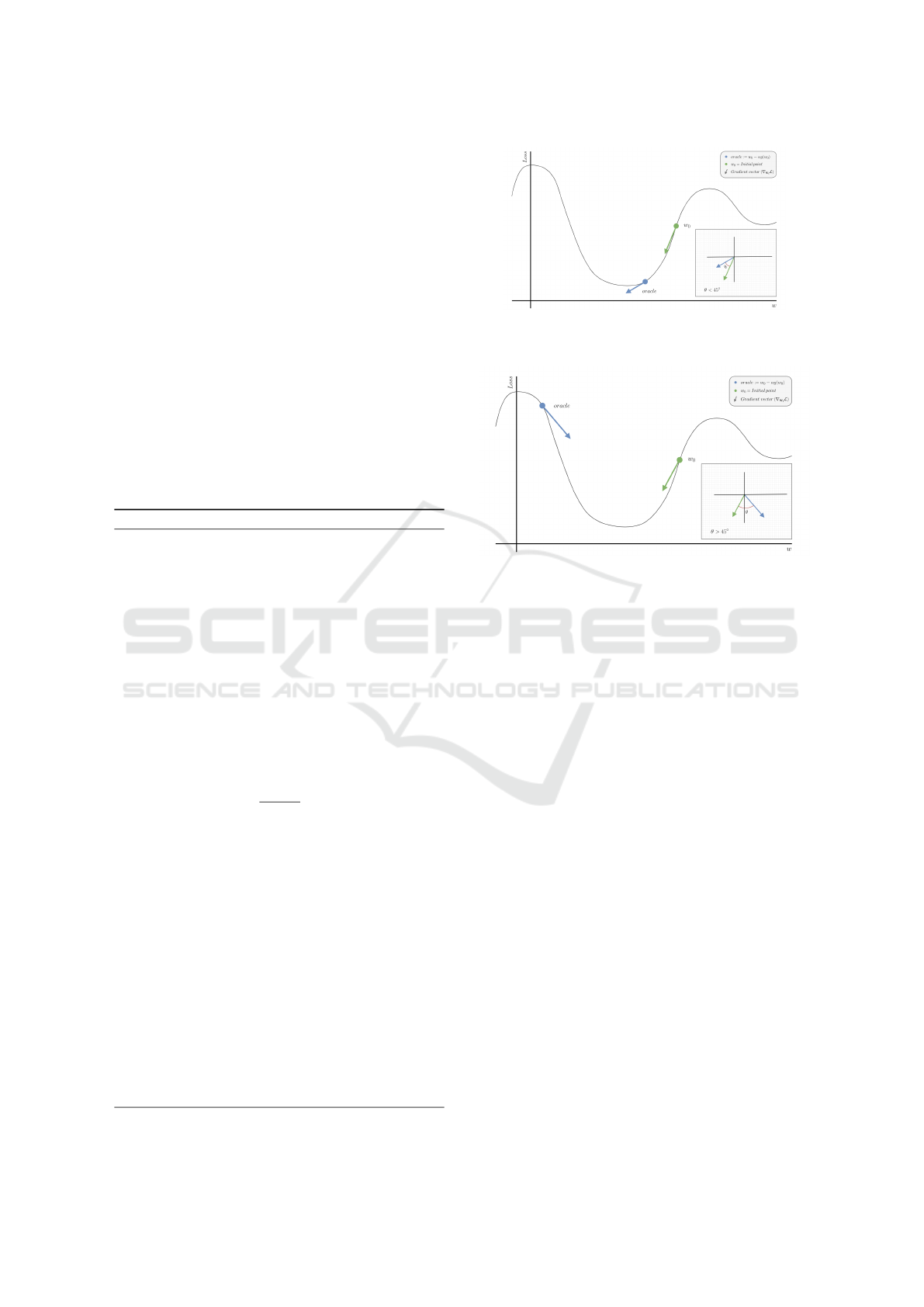
(a) The weight update results in both the previous weight w

and the oracle to be on the same side of the loss surface. In

such case, the ﬁrst if statement would be evaluated as False.

(b) The weight update results in the oracle bouncing off

from the side where the previous weight w

was on the loss

surface. In such case, the ﬁrst if statement would be evalu-

ated as True.

Figure 1: An elementary example to showcase the two pos-

sible cases of the ﬁrst if statement in Algorithm 1.

As presented in Algorithm 1, BGD leverages rel-

atively signiﬁcant step sizes in order to maximize its

regional search in the weight space for a generalizable

set of weights that coincide with a ﬂatter local mini-

mum in the ﬁtness landscape. The ﬁrst if statement

is used to determine whether the optimizer’s initial

weight update: oracle = w

−α ⊙g

has caused the or-

acle to bounce off from one side of the loss surface to

another, indicated by the vector dot product

⟨

, g

orc

⟩

being non-positive. Additionally, we provide several

ﬁgures to help visualize the geometry of the dot prod-

uct if condition, as well as the possible trajectory dy-

namics that BGD can follow. Figure 1 presents a sim-

pliﬁed illustrative example, showcasing the two pos-

sible conditions of the ﬁrst if statement.

Additionally, since BGD is an adaptive algorithm

(based on the second moment of gradients) that de-

ploys per-parameter step sizes, we explicitly capture

this notion in the step size α hyperparameter. Where

α is now a vector with relatively large step sizes cor-

responding to each weight, and the adaptivity of these

step sizes will become apparent when the second if

statement in Algorithm 1 is ﬁrst triggered, speciﬁcally

when α = α/υ

t+1

, indicating an element-wise divi-

sion.

BGD: Generalization Using Large Step Sizes to Attract Flat Minima

243

Furthermore, the dist function is a vector-valued

distance-measuring (score) function that serves the

purpose of evaluating the relative quality of the two

given gradient vectors in order to yield two respective

distances summing up to one; resembling a weighted

sum of distances corresponding to each gradient vec-

tor.

The quality of a gradient degrades as its vector

norm increases and vice versa; here, the L2 norm was

used for the evaluation. A weight vector that yields a

smaller gradient norm will result in a comparatively

large distance value, and hence; the weight update

will lean closer towards that weight vector, allow-

ing the optimizer to quickly jump to attracting basins

given the large step sizes. The dist function can take

many forms, though the formulation used for the dist

function in the experiments was a simple and straight-

forward one, taking the following form:

dist (g

, g

) = [



∥



+ ε

∥



+ ε

(11)

where for numerical stability purposes, ε > 0 is a

small value added to the denominator. The thresh-

old value τ is an additional tunable hyperparameter

in BGD that determines when to adaptively shrink the

value of the step size vector α based on the second

moment of gradients υ in order to stabilize the future

weight updates. Execution of the second if statement

indicates that the overshooting oracle has landed on

a loss surface with a sharp (steep) curvature as com-

pared to its previous point w

, characterized by a large

gradient norm, and thus; the d

value corresponding to

will be relatively large. Hence, using a low thresh-

old value will be more suitable for highly non-convex

surfaces, as it will cause the second if statement to

trigger more often, consequently reducing the over-

all step size vector α. In practice, a threshold value

of τ ∈ [0.7, 0.9] was determined to work best empiri-

cally.

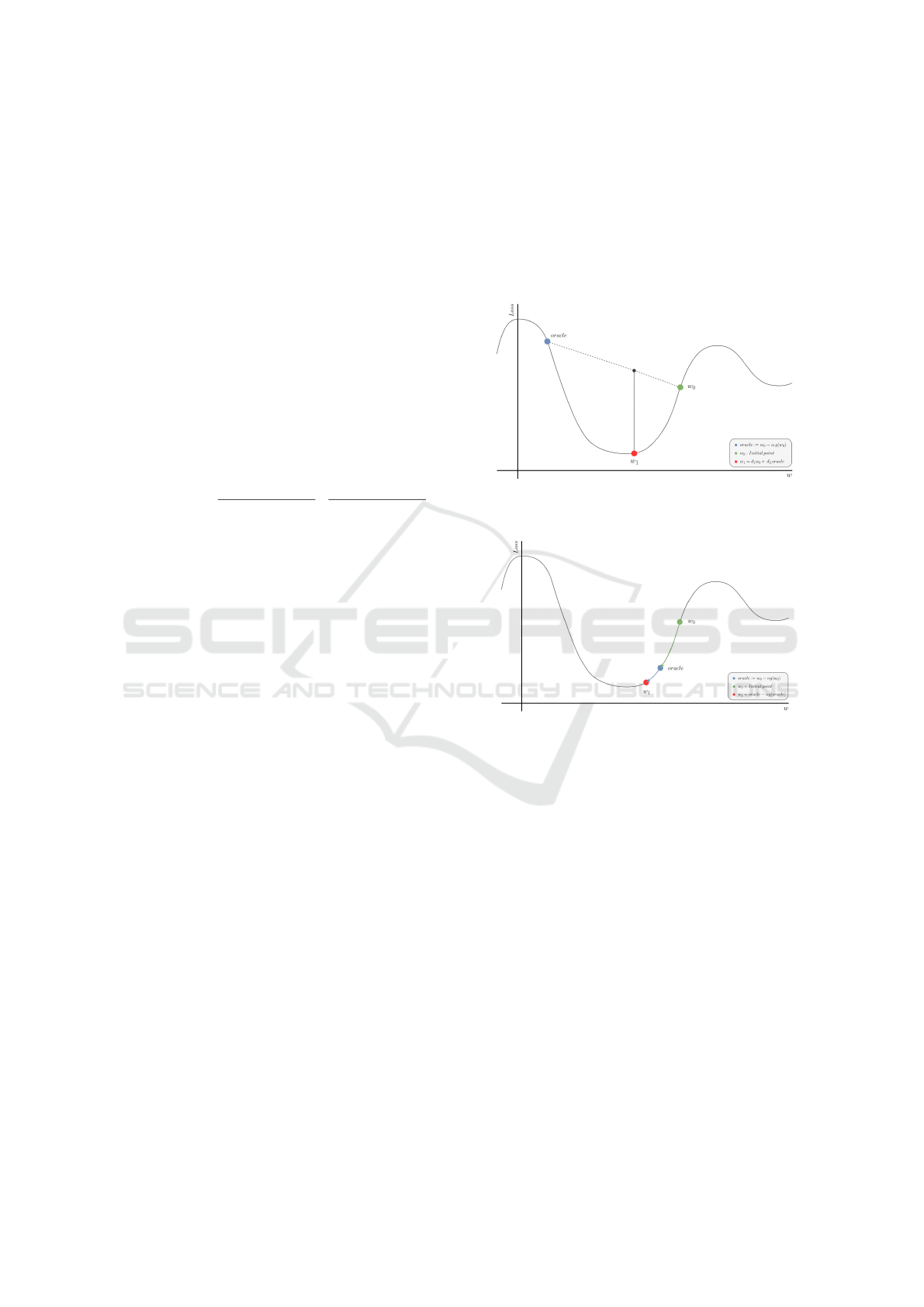
As apparent in Algorithm 1, BGD contains two

versions of the weight update. Where if the ﬁrst if

statement was triggered, the ﬁrst version of the form

t+1

= d

·w

+ d

·oracle will occur; implying that

the oracle has bounced off from the side of the loss

surface where the previous weight w

was at. The

updated weight w

t+1

in the ﬁrst version will be a

weighted average of previous weight w

and the or-

acle, causing w

t+1

to land somewhere in between the

two valleys around the loss basin. However, if the ﬁrst

if statement was not triggered, the second version of

the weight update will take place, which basically is

a gradient descent step from the oracle’s position to-

wards the local minimum. Both versions of the weight

update are illustrated in Figure 2.

Finally, since the step size for BGD does not need

to decay continuously to achieve stable convergence

as it does for SGD, allowing for a relatively large step

size to be utilized, which in turn leads to faster con-

vergence and the potential to converge to ﬂatter lo-

cal minima due to the random exploration of the loss

landscape.

(a) Description of the ﬁrst version of the weight update

which is applied when the ﬁrst if statement is evaluated as

True.

(b) Description of the second version of the weight update

which is applied when the ﬁrst if statement is evaluated as

False.

Figure 2: A simpliﬁed example that demonstrates the two

versions of the weight update presented in Algorithm 1.

4 EXPERIMENTATION AND

RESULTS

To begin, a comparison between GD and BGD is

made in terms of minimizing a simple β-smooth α-

strongly convex quadratic function f : R

→ R for

ﬁve iterations, in order to demonstrate the behavior

of the paths taken by each algorithm across differ-

ent step size values. As shown in the contour plots

of Figure 3, when a relatively proper step size is cho-

sen, GD weight updates follow a smooth trajectory to-

ward the minimum point of the function. Even though

this choice of step size does not fully capitalize on the

bouncing properties of BGD, it still manages to out-

perform GD signiﬁcantly thanks to its advantageous

VISAPP 2023 - 18th International Conference on Computer Vision Theory and Applications

244

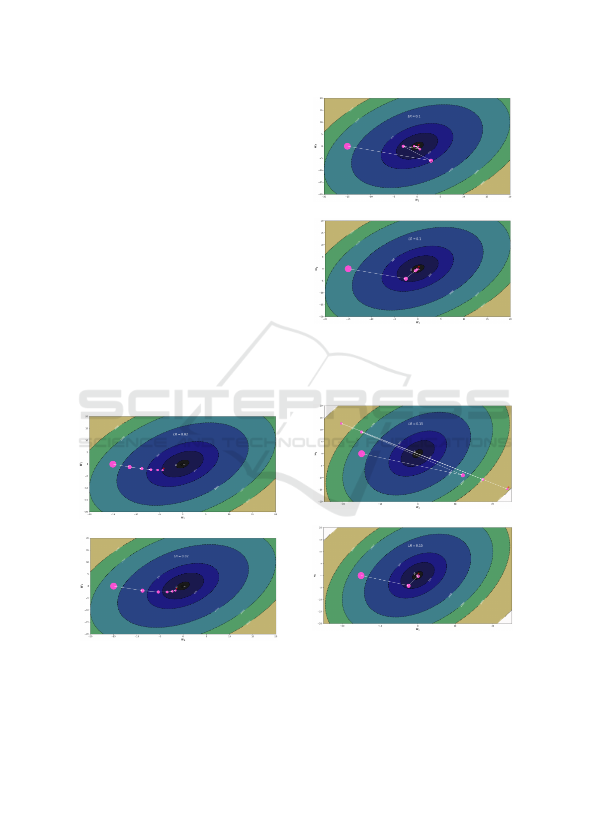
use of oracles. Figure 4 depicts the same comparison

made between the two algorithms, but this time, we

opted for a comparatively larger step size than the one

in Figure 3. As a result, we can see GD starting to

demonstrate oscillating behavior caused by bounces

around the basin of the function’s local minimum, in-

dicating that GD’s weight updates are overshooting

the minimum. On the other hand, BGD managed not

to overshoot the function’s minimum and bounce off

to the other side due to its utilization of the ﬁrst ver-

sion of the weight update in BGD, resulting in faster

and more stable convergence.

Finally, Figure 5 shows the most unfavorable case

for GD, yet the most favorable case for BGD, where

a relatively large step size is deployed. Consequently,

GD started diverging away from the function’s

minimum and would require additional manual

intervention in order to stabilize its weight updates by

incorporating a step size decay per iteration. Again,

however, BGD faces no issues and is successfully

able to leverage the large step size to its advantage,

converging stably in much fewer steps than usual.

Furthermore, surprisingly, BGD is able to handle

much larger step sizes than those used in the ﬁgures.

However, when using such step sizes, GD starts to

diverge heavily and goes beyond the visible bounds

of the contour plots.

(a) Trajectory of the weight updates taken by GD.

(b) Trajectory of the weight updates taken by BGD.

Figure 3: A comparison between the trajectories taken

by GD versus BGD when minimizing the function:

f (w

, w

) = 6w

+ 4w

−4w

using a relatively small

step size of 0.02. The the ﬁnal point is represented by the

asterisk symbol.

(a) Trajectory of the weight updates taken by GD.

(b) Trajectory of the weight updates taken by BGD.

Figure 4: A comparison between the trajectories taken by

GD and BGD when minimizing the function: f (w

, w

) =

+ 4w

− 4w

using a relatively modest step size

(learning rate) of 0.1. The the ﬁnal point is represented by

the asterisk symbol.

(a) Trajectory of the weight updates taken by GD.

(b) Trajectory of the weight updates taken by BGD.

Figure 5: A comparison between the trajectories taken by

GD and BGD when minimizing the function: f (w

, w

) =

+4w

−4w

using a relatively large step size (learn-

ing rate) of 0.15. The the ﬁnal point is represented by the

asterisk symbol.

BGD: Generalization Using Large Step Sizes to Attract Flat Minima

245

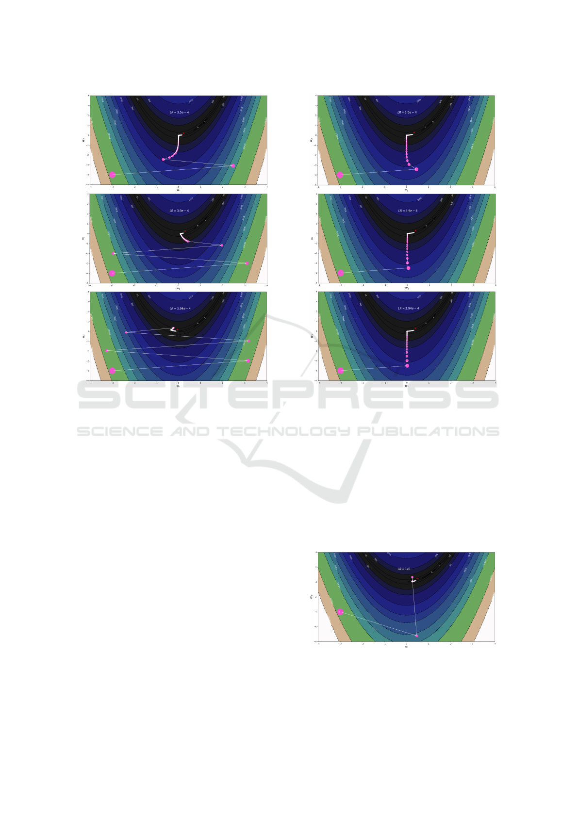
Figure 6: The trajectories taken by GD when minimizing

the Rosenbrock function: f (x, y) = (1 −x)

+100



y −x



across different values of the step size hyperparameter α,

where the ﬁnal point is represented by the asterisk symbol.

In addition, a comparison of the trajectory dynam-

ics of both algorithms GD and BGD on minimizing

the Rosenbrock function f : R

→R for 325 iterations

is conducted. The Rosenbrock function is unimodal,

and its global minimum lies in a narrow, parabolic

valley, which is notoriously difﬁcult to converge to

for gradient-based optimization algorithms. As shown

in Figure 6, GD’s convergence performance deterio-

rates as the step size increases due to the oscillations

around the valley of the function, failing to utilize the

increase in step size when approaching the minimum

of the Rosenbrock function. Moreover, GD’s conver-

gence performance is extremely sensitive to the step

size used, as relatively small adjustments made to the

step size result in extreme changes in the trajectories

and convergence of GD due to the non-convexity of

the Rosenbrock function. On the other hand, as illus-

trated in Figure 7, BGD’s convergence actually im-

proves as the step size increases, since BGD is able

to quickly land in the valley of the Rosenbrock func-

tion thanks to its ﬁrst version of the weight update

(illustrated in Figure 2 (a)). Another important thing

to note is that GD started to diverge to inﬁnity when

Figure 7: The trajectories taken by BGD when minimizing

the Rosenbrock function: f (x, y) = (1 −x)

+100



y −x



across different values of the step size hyperparameter α,

where the ﬁnal point is represented by the asterisk symbol.

the step size was slightly altered to 3.95e−4, while

conversely, BGD demonstrated faster convergence to-

wards the minimum.

Furthermore, BGD can handle exceptionally large

step sizes, achieving remarkable performance even

when using a step size of α =1e5, resulting in a solu-

tion with a function value of 0.319 in 325 iterations as

demonstrated in Figure 8 This shows that even while

algorithm tested for the extreme cases gives stable

Figure 8: The trajectories taken by BGD when minimizing

the Rosenbrock function: f (x, y) = (1 −x)

+100



y −x



using an exaggerated value of 100000 for the step size hy-

perparameter α, where the ﬁnal point is represented by the

asterisk symbol.

VISAPP 2023 - 18th International Conference on Computer Vision Theory and Applications

246

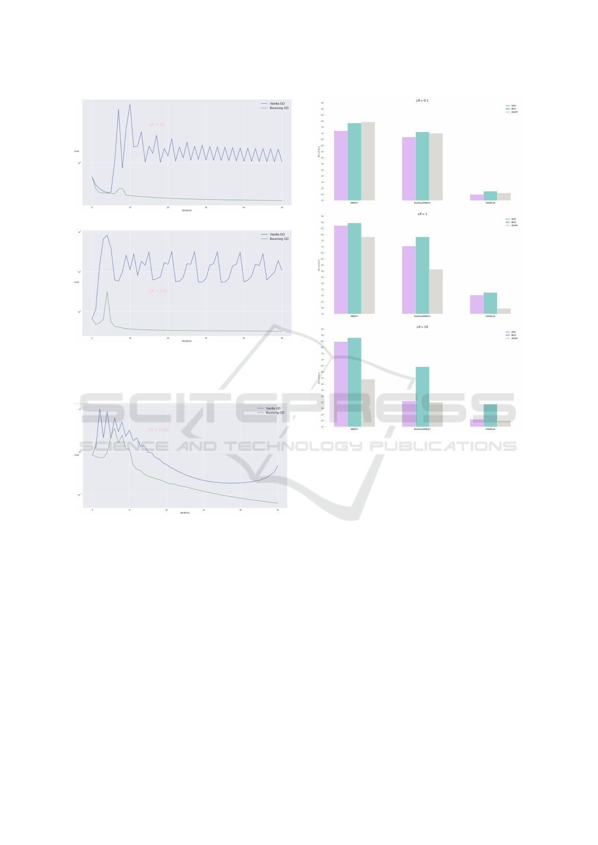
(a) Minimizing the logistic loss using a step size of 10.

(b) Minimizing the logistic loss using a step size of 100.

Figure 9: The log-scaled loss curves of each algorithm when

minimizing the logistic loss on the a1a dataset using two

different step sizes (learning rates).

Figure 10: The log-scaled loss curves of each algorithm

when minimizing the logistic loss on the news.20.binary

dataset using an exaggerated step size (learning rate) of

1000.

performance and it doesnot crash.

Next, we demonstrate yet another optimization

comparison between GD and BGD, though this time,

by observing how each algorithm minimizes the

logistic loss on two different binary classiﬁcation

datasets taken from the LIBSVM library (Chang and

Lin, 2011). The ﬁrst dataset is the simple a1a dataset,

which consists of 1,605 training examples, where

each example contains 123 input features. Figure 9 il-

lustrates the loss curves generated by training on each

algorithm. The second dataset is the more extensive

news.20.binary dataset, which contains 19,996 train-

ing examples and 1,355,191 input features per exam-

Figure 11: The classiﬁcation accuracy of the different opti-

mization algorithms evaluated on multiple benchmark clas-

siﬁcation datasets when using a batch-size of 1000.

ple. Its loss curves are depicted in Figure 10; even

though both algorithms suffered from loss oscillations

initially, they eventually managed to ﬁnd a relatively

smoother loss surface. However, GD started diverging

towards the end of the training phase, indicating that

the attracting basin of the loss function’s local min-

imum was relatively sharp; hence, GD bounced off

the minimum’s basin which resulted in a cascading

diverging effect, because unlike BGD, GD is unable

to handle large values of the step size α. Therefore

we cannot use very large learning rates with GD as it

will crash. While for the case of BGD we prove the

handling of even large learning rates with improved

convergence. That shows consistent performance of

our algorithm.

Finally, we conducted classiﬁcation performance

comparisons between SGD (with and without mo-

mentum), BGD, and ADAM on popular benchmark

image classiﬁcation datasets by minimizing the cate-

gorical cross-entropy loss of a three-layer non-linear

feedforward neural network, also known as a multi-

BGD: Generalization Using Large Step Sizes to Attract Flat Minima

247

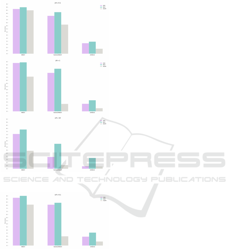
Figure 12: The classiﬁcation accuracy of the different opti-

mization algorithms evaluated on multiple benchmark clas-

siﬁcation datasets when using a batch-size of 100.

Figure 13: The classiﬁcation accuracy of the different opti-

mization algorithms evaluated on multiple benchmark clas-

siﬁcation datasets when using a batch-size of 10.

layer perceptron (MLP). For SGD, the best result be-

tween SGD versus SGD with momentum was cho-

sen for SGD’s performance evaluation. Each opti-

mizer was run using the same weight initialization,

same number of epochs, identical learning rates in

each run, and with the proper image normalization for

each dataset. Moreover, all the experiments were run

for ﬁve epochs while using the tanh non-linear acti-

vation for the hidden layers of the NN (other activa-

tion functions where also used such as ReLU and sig-

moid in the Appendix). Firstly, in Figure 11, a batch-

size of 1000 was used across different step sizes to

demonstrate each algorithms performance when uti-

lizing relatively stable gradients. Secondly, in Figure

12, a batch-size of 100 was used across different step

sizes, and ﬁnally, in Figure 13, a small batch-size of

10 was used with a relatively small learning rate to

demonstrate each algorithms performance when deal-

ing with comparatively high-variance (noisy) gradi-

ents. As illustrated in all the Figures, BGD consis-

tently outperforms both GD and ADAM under all set-

tings, and speciﬁcally, when a relatively large step

size is used, conﬁrming BGD’s superiority in utilizing

large step sizes. This algorithm shows stable perfor-

mance in all the different settings shown and proved

the usefulness of this algorithm. With better and opti-

mized learning rates this algorithm can be utilized for

downstream tasks with improved convegence.

5 CONCLUSION

The primary goal of this paper was to tackle the sig-

niﬁcantly practical problem of being able to train

a generic model that can generalize efﬁciently by

learning predictive knowledge from a limited train-

ing dataset, given that the gathered data is not a sta-

tistically signiﬁcant representation of the population

data due to selection bias. We introduced the BGD al-

gorithm, a novel and robust gradient-based optimiza-

tion algorithm aimed at capturing ﬂatter local min-

ima as compared to SGD and its variants for non-

convex objective functions. The BGD algorithm is

constructed in such a way as to leverage relatively

large step sizes to its advantage since the step size re-

stricts the set of local minima that the algorithm can

converge to, allowing the optimizer to better explore

the loss landscape in search of a ﬂatter set of local

minima. BGD also makes use of overshooting ora-

cles, which enable the optimizer to bounce across the

loss landscape’s basins and avoid as many undesir-

able sharp local minima as possible in order to eventu-

ally settle on a sufﬁciently ﬂat local minimum, which

induces model generalizability. This paper also aims

to push for intuitive, unorthodox approaches that uti-

lize large step sizes in weight updates to balance the

variance-stability ∼ exploration-exploitation tradeoff.

Currently, most proposed SGD variants rely heavily

on exploiting the local information about the loss sur-

face to stabilize training and convergence rather than

utilizing the inherent variance advantageously to fur-

ther explore the loss landscape, exposing the opti-

VISAPP 2023 - 18th International Conference on Computer Vision Theory and Applications

248

mizer to a broader set of minima in the hopes of at-

tracting a ﬂatter local minimum. The experimenta-

tions conducted empirically validate the superiority

and consistency of the proposed algorithm over the

baseline methods in improving classiﬁcation accuracy

and achieving model generalization. They also reveal

the robustness of BGD and demonstrate that it is well-

suited to a wide range of non-convex optimization

problems in machine learning.

REFERENCES

Ben-David, S., Blitzer, J., Crammer, K., Kulesza, A.,

Pereira, F., and Vaughan, J. W. (2010). A theory of

learning from different domains. Machine learning,

79(1):151–175.

Cha, J., Chun, S., Lee, K., Cho, H.-C., Park, S., Lee, Y.,

and Park, S. (2021). Swad: Domain generalization by

seeking ﬂat minima. Advances in Neural Information

Processing Systems, 34:22405–22418.

Chang, C.-C. and Lin, C.-J. (2011). LIBSVM: A library for

support vector machines. ACM Transactions on Intel-

ligent Systems and Technology, 2:27:1–27:27. Soft-

ware available at http://www.csie.ntu.edu.tw/

∼

cjlin/

libsvm.

Dauphin, Y. N., de Vries, H., Chung, J., and Ben-

gio, Y. (2015). Rmsprop and equilibrated adaptive

learning rates for non-convex optimization. CoRR,

abs/1502.04390.

Defazio, A., Bach, F., and Lacoste-Julien, S. (2014). Saga:

A fast incremental gradient method with support for

non-strongly convex composite objectives. Advances

in neural information processing systems, 27.

He, H., Huang, G., and Yuan, Y. (2019). Asymmetric val-

leys: Beyond sharp and ﬂat local minima. Advances

in neural information processing systems, 32.

Izmailov, P., Podoprikhin, D., Garipov, T., Vetrov, D., and

Wilson, A. G. (2018). Averaging weights leads to

wider optima and better generalization. arXiv preprint

arXiv:1803.05407.

James, G., Witten, D., Hastie, T., and Tibshirani, R. (2013).

An introduction to statistical learning, volume 112.

Springer.

Johnson, R. and Zhang, T. (2013). Accelerating stochastic

gradient descent using predictive variance reduction.

Advances in neural information processing systems,

26.

Keskar, N. S., Mudigere, D., Nocedal, J., Smelyanskiy, M.,

and Tang, P. T. P. (2016). On large-batch training for

deep learning: Generalization gap and sharp minima.

arXiv preprint arXiv:1609.04836.

Kingma, D. P. and Ba, J. (2014). Adam: A method

for stochastic optimization. arXiv preprint

arXiv:1412.6980.

Kone

y, J. and Richt

arik, P. (2013). Semi-stochastic gradi-

ent descent methods. arXiv preprint arXiv:1312.1666.

Lengyel, D., Jennings, N., Parpas, P., and Kantas, N. (2021).

On ﬂat minima, large margins and generalizability.

Nar, K. and Sastry, S. (2018). Step size matters in deep

learning. Advances in Neural Information Processing

Systems, 31.

Netrapalli, P. (2019). Stochastic gradient descent and its

variants in machine learning. Journal of the Indian

Institute of Science, 99(2):201–213.

Neyshabur, B., Li, Z., Bhojanapalli, S., LeCun, Y., and Sre-

bro, N. The 1359 role of over-parametrization in gen-

eralization of neural networks. In International, vol-

ume 1360.

Nguyen, L. M., Liu, J., Scheinberg, K., and Tak

c, M.

(2017). Sarah: A novel method for machine learning

problems using stochastic recursive gradient. In In-

ternational Conference on Machine Learning, pages

2613–2621. PMLR.

Ruder, S. (2016). An overview of gradient de-

scent optimization algorithms. arXiv preprint

arXiv:1609.04747.

Simsek, B., Ged, F., Jacot, A., Spadaro, F., Hongler, C.,

Gerstner, W., and Brea, J. (2021). Geometry of the

loss landscape in overparameterized neural networks:

Symmetries and invariances. In International Confer-

ence on Machine Learning, pages 9722–9732. PMLR.

Wen, W., Wang, Y., Yan, F., Xu, C., Wu, C., Chen, Y., and

Li, H. (2018). Smoothout: Smoothing out sharp min-

ima to improve generalization in deep learning. arXiv

preprint arXiv:1805.07898.

BGD: Generalization Using Large Step Sizes to Attract Flat Minima

249