Popularity Prediction for New and Unannounced Fashion Design

Images

Danny W. L. Yu

, Eric W. T. Ngai

and Maggie C. M. Lee

Department of Management and Marketing, The Hong Kong Polytechnic University, Hung Hom, Hong Kong

Keywords: Popularity, Attractiveness, Fashionability, Multi-Layer Perceptron Regression, Convolutional Neural

Network (CNN).

Abstract: People following the latest fashion trends gives importance to the popularity of fashion items. To estimate

this popularity, we propose a model that comprises feature extraction using Inception v3 (a kind of

Convolutional Neural Network) and a popularity score estimation using Multi-Layer Perceptron regression.

The model is trained using datasets from Amazon (5,166 items) and Instagram (98,735 items) and evaluated

by using mean-squared error, which is one of the many metrics of the performance of our model. Results

show that, even with a simpler structure and requiring less input, our model is comparable with other more

complicated methods. Our approach allows designers and manufacturers to predict the popularity of design

drafts for fashion items, without exposing the unannounced design at social media or comparing with a large

quantity of other items.

1 INTRODUCTION

The ability to know the next popular type of clothes

is highly prized for the fashion industry. By

successfully forecasting how likely customers may

buy pieces of clothing during the design process,

designers can make the most of resources to

manufacture the best-received styles, meeting heavy

demands and avoiding the waste of time and labor on

those that may have less sales. However, as fashion

tastes vary from person to person, these predictions

are often made under the influence of personal

preferences and are thus predominantly subjective.

To facilitate such prediction in a quantitative and

more objective manner, Simo-Serra et al. (2015) and

Wang et al. (2015), among others, devised fashion

popularity prediction models for assessing which

outfits are more “attractive”, “fashionable”, or “likely

to receive likes”. Despite such attempts, many

limitations remain. These models rely solely on

statistics from social media platforms, which may

mainly reflect the attractiveness of photography

styles and users who post the photos, instead of the

attractiveness of the fashion item itself. In addition,

https://orcid.org/0000-0002-5362-6547

https://orcid.org/0000-0001-6891-6750

https://orcid.org/0000-0002-5572-5629

these models ignore the sales that reflect the product

attractiveness to the market. In addition, several

models may pose operational issues by merely

comparing the popularity between clothes but not

providing a concrete index (Wang et al., 2015) or the

required input (e.g., number of comments, number of

followers) that are not available until its posting on

social media (Simo-Serra et al., 2015). Therefore,

these models are unsuitable to predict new and

unannounced fashion items to be sold in the market.

Based on our research problem and literature review,

we identify and articulate the need for such methods

that can meet the needs of fashion designers and

manufacturers, thereby motivating this study and

leading to the question: how can we predict

popularity of new fashion images to be sold in the

market?

Therefore, this study proposes a novel method to

measure the popularity score of a fashion item by

considering data from both e-commerce and social

media platforms. The model comprises feature

extraction and regression modules, which accept an

image of clothing and returns a numeral popularity

score. The eased input requirements make this model

Yu, D., Ngai, E. and Lee, M.

Popularity Prediction for New and Unannounced Fashion Design Images.

DOI: 10.5220/0011768500003393

In Proceedings of the 15th International Conference on Agents and Artiﬁcial Intelligence (ICAART 2023) - Volume 3, pages 729-736

ISBN: 978-989-758-623-1; ISSN: 2184-433X

 2023 by SCITEPRESS – Science and Technology Publications, Lda. Under CC license (CC BY-NC-ND 4.0)

729

suitable for estimating the popularity of a draft design

for fashion designers, without the need of evaluating

the responses from social media platforms (which can

lead to design copies) or comparing with a large

quantity of other items (which is computationally

inefficient and raises fairness issues).

The rest of this paper is arranged as follows.

Section 2 summarizes the related works and

highlights their current limitations. Section 3

elaborates on how the method evaluates the image

popularity of an outfit, and Section 4 explains our

model architecture. Section 5 evaluates the model

using datasets and discusses the effects of several of

our design choices. The study is finally summarized

in Section 6.

2 RELATED WORKS

In this section, we discuss two areas of literature that

are related to the current study, namely, fashion

popularity prediction and fashion recommendation.

2.1 Fashion Popularity Prediction

In predicting whether an outfit can be trending or

popular, the most commonly used indicator is the

number of likes received in social networks. In social

media, users that find a post interesting can leave

“likes”. This measure often exhibits a long tailed

distribution, and thus the common practice is to

perform a logarithmic transform before further

processing, as in Simo-Serra et al. (2015) and Lo et

al. (2019).

Simo-Serra et al. (2015) investigated the

relationship between “fashionability”, defined based

on the number of likes received by a post on a

fashion-dedicated social media network named

Chictopia, and the information from the post. In their

work, they created a Conditional Random Field

model that predicts “fashionability” by using a score

from 0 to 10 on factors ranging from the attributes of

the clothes (e.g., color, garment) to contextual

information (e.g., the follower count and location of

the poster). Although this previous study laid the

foundation of many fashion popularity prediction

models, the measure relies heavily on the tags

provided by users but neglects the images themselves.

As such, several more intricate visual patterns on the

clothes can be missed out in the prediction. Wang et

al. (2015), given a pair of garment images, report

which one is expected to receive more likes on social

media platforms. The method considers the

appearance and visual attributes of the outfit and

predicts which image can receive more likes by using

classification and feature extraction. Based on the

classification labels and deep features of the image,

the method deduces which one is more “attractive”

using Sum Product Network. While this previous

work provides a means to compare fashion images,

the method becomes inefficient when the number of

images increases due to the required pairwise

comparison. Lo et al. (2019) feature a model that, in

addition to the deep image feature and garment type,

considers the chronological order of social media

posts. Thus, this sequential model accepts—instead

of a single image and its meta-data—a series of

images and their garment types, ordered by time and

with the number of likes known for all images except

the last, which the model aims to predict. However,

all the abovementioned works ignore the sales records

that reflect the attractiveness of products to the

market.

2.2 Fashion Recommendation

Another area of related work, albeit distantly, is

fashion recommendation. The goal of this type of

system is to recommend an outfit that is in line with

trends, or in which users may be interested. Simo-

Serra et al. (2015) suggest the types and colors of

clothing and accessories that the poster may have

worn by formulating the recommendation as a

maximization problem of “fashionability” score. As

their model predicts scores using the clothing

attribute labels, the system tests each garment-related

attribute and finds those with the best scores.

In enabling personalized recommendations, these

systems consider user preferences in the form of

ratings to other outfits or purchase history, in addition

to image features and/or their description. The

simplest systems can be designed using collaborative

filtering techniques, such as Singular Value

Decomposition. One sophisticated model is that of

Kang et al. (2017), who extract the image features

using the Siamese Convolutional Neural Network and

recommend items using Bayesian Personalized

Ranking model trained on the review histories and

interaction logs from e-commerce platforms along

with the item images. Zhang and Caverlee (2019)

recommend a time-aware model based on Recurrent

Recommendation Network and consider the users’

review history on Amazon with pictures of fashion

influencers on Instagram. However, these works

recommend for individuals based on personal

preferences only but do not predict the popularity.

ICAART 2023 - 15th International Conference on Agents and Artiﬁcial Intelligence

730

3 FASHION POPULARITY

PREDICTION

3.1 Problem Definition

In this study, we consider fashion popularity

prediction for the overall score of a fashion item, in

which the score reflects the sales, such as count and

ranking in e-commerce websites, and the number of

likes and comments on social media platforms. This

score ranges from 0 to 1 as the least and most popular,

respectively. This scoring naturally fits our model.

The scoring scheme is further explained in the next

section. Specifically, given an image I and its garment

type, we predict the popularity score 𝑠



 , which must

be as close as the actual popularity score 𝑠



3.2 Score Calculation

As the data from different sources have different

measures of popularity, we have different formulae to

evaluate the scores. Despite the difference in data

availability between each source, the scoring scheme

yields a single numeral output, and thus data from

different kinds can be combined. Fairness across

different platforms is attained by calibrating the

scores to align the mean and standard deviation. Our

scoring method is inspired by Simo-Serra et al. (2015)

and their logarithmic transform followed by

bucketing and fitting the data into a normal

distribution. Although we adopt the Gaussian

distribution to facilitate training, we set the score to a

continuous range of (0, 1) instead of their integer

range [1…10]. This section elaborates on the

calculation and combination methods.

3.2.1 e-Commerce-Based Scores

For the items from the e-commerce platforms, we

consider the sales rank, average review scores, and

the review count. The contribution to sales rank is

evaluated using the formula:

𝑆



=max



1 −

𝑅

𝑇

, 0



∈



0,1



(1)

where R is the rank of the item and T is the threshold.

We adopt a normalization approach by standardizing

the average review scores followed by a transform

using the cumulative distribution function (CDF) of

the normal distribution. Thus, the score is mapped

back to the range (0, 1). Formally, the formula is:

𝑆



= Φ

𝑟−𝑟

𝑠





(2)

where 𝑟 is the average score of the item; 𝑟̅ and 𝑠



are

the mean and standard deviation of the average

review score across all items in the dataset,

respectively; and Φ is the CDF of standard normal

distribution, namely:



𝑥



√

2𝜋

𝑒









𝑑𝑡





(3)

We use a similar normalization for the review

count component and other count-based metrics.

However, compared with the review score, such

metrics exhibit long tailed distributions. Therefore,

we perform a natural logarithmic transform

beforehand. Formally, for the count metric c:

c′=ln



𝑐+1



(4)

𝑆



= Φ

𝑐′−c





𝑠







(5)

where 𝑐





and 𝑠





are the mean and standard deviation

respectively of the count metric after

logarithmic transform. The overall score for an item

from an e-commerce platform is the weighted sum of

these factors, specifically,

𝑆



= 𝑤



𝑆



+ 𝑤



𝑆



+ 𝑤



𝑆



(6)

with 𝑤



+ 𝑤



+ 𝑤



=1 to fix the score in

the range (0,1).

3.2.2 Social Media-Based Scores

For items from social media posts, we adopt the

number of likes and comments as metrics for

popularity. The calculation methods for both

components are the same as that of the review score

for the e-commerce items. The overall score for an

image from a social media platform is calculated as

𝑆





= 𝑤



𝑆



+ 𝑤



𝑆



(7)

with 𝑤



+ 𝑤



=1.

3.2.3 Incorporating the Two Scores

To incorporate the different scores from different

sites, we adjust the mean and standard deviation of

the social media datasets to match those of e-

commerce platforms and clamp the scores to the

range (0, 1). Formally, we use the following formula

to shift the distribution of the two datasets:

𝑆



=minmax 

𝑠







𝑠





∙𝑆





−𝑆









+ 𝑆





,1,0

(8)

Popularity Prediction for New and Unannounced Fashion Design Images

731

where 𝑠







and 𝑠





are standard deviations of

unadjusted social media scores and e-commerce

scores respectively.

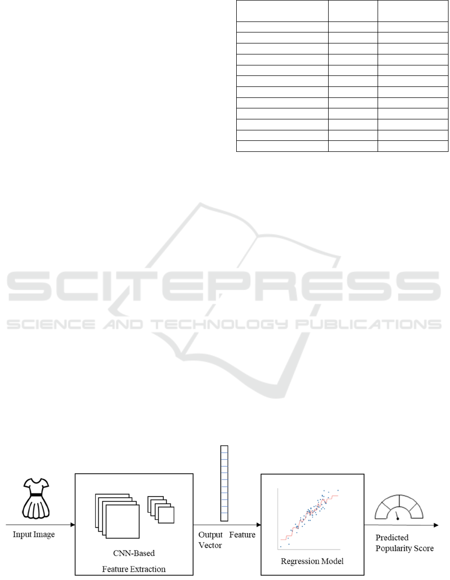
4 PROPOSED METHOD

In this study, we propose a model that comprises

feature extraction and regression modules, which

accept an image of clothing and return a numeral

popularity score, as outlined in Figure 1. We use a

modified Inception v3, a Convolutional Neural

Network architecture proposed by Szegedy et al.

(2016), as our feature extraction module, while the

second last layer of Inception v3 is used as an output

feature vector representing the image. This feature

vector is then fit into a regression model database to

estimate the popularity score. In the following

subsections, the feature extraction and score

prediction methods are described in detail.

4.1 Feature Extraction

The first part of our model (

Table 1

) extracts and thus

“perceives” the “features” from images. This process,

usually implemented by Convolutional Neural

Network, is known as feature extraction, which takes

a bitmap image as input and returns several vectors.

Our feature extraction method is based on the

Inception v3 model, with its structure shown in Table

1. We fine-tuned a pre-trained model from PyTorch

model zoo, Inception v3 introduced by Szegedy et al.

(2016) and trained it on the FashionMNIST dataset

(Xiao et al., 2017). Despite its inclusion of images of

different types of garments, this dataset does not

sufficiently provide responses on the details of the

clothing items. Therefore, we fine-tuned the model

using our dataset to improve the quality while saving

on training time.

Table 1: Structure of modified Inception v3 used, excerpted

from Szegedy et al. (2016).

Type of Layer

Patch Size

/ Stride

Input Size

Convolution 3×3/2 299×299×3

Convolution 3×3/1 149×149×32

Convolution Padde

3×3/1 147×147×32

Pooling 3×3/2 147×147×64

Convolution 3×3/1 73×73×64

Convolution 3×3/2 71×71×80

Convolution 3×3/1 35×35×192

3×Ince

tion 35×35×288

5×Inception 17×17×768

2×Inception 8×8×1280

Poolin

8×8 8×8×2048

Out

ut 2048

To obtain the feature vector, we need to modify

the network structure, which serves as a classifier of

1,000 classes; thus, its final fully connected layer has

1,000 output features. However, we are not bound to

the classes of the original dataset. The final layer is

not necessary, and the result of the second final layer

can be taken as the output image feature vector.

4.2 Score Prediction

The feature vector is then fed to the regression, with

the core assumption that clothes similar to popular

outfits are more likely to be popular. This model

remembers the feature vectors and its prediction

scores. Then, the model compares the input and the

known feature vectors and returns the average of the

score associated with the closest ones to provide a

prediction. Such comparison can be made for each of

the 2,048 dimensions, or holistically as the Euclidean

distance in k-Nearest Neighbor (kNN) regression.

Figure 1: The architecture diagram of the proposed method.

ICAART 2023 - 15th International Conference on Agents and Artiﬁcial Intelligence

732

In this study, the selected regression model is

Multi-Layer Perceptron (MLP) based on a neural

network, after a series of experiments documented in

the next section. We use scikit-learn, a software

machine learning library tool for predictive data

analysis of the regression model.

5 EXPERIMENTS AND RESULTS

5.1 Dataset and Experimental Setting

In our experiment, we use two datasets, namely, from

an e-commerce and a social media platform. Thus, the

datasets can reflect the trends of both sources, which

often exhibit different tastes and preferences. Dress

and blouse images are selected from the databases,

and the numbers of images used in Amazon and

Instagram datasets are 5,166 and 98,735,

respectively.

5.1.1 Dataset from Amazon

The e-commerce dataset is derived from McAuley et

al. (2015). Data on sales ranks, descriptions, and

prices of the items sold on Amazon are provided

along with their reviews, which include the reviewer

ID, score, and a timestamp of the user comment. In

which, the clothing and jewelry parts of the dataset

comprise the information of 1.5 million items and

5.74 million ratings. Given the scope of this study, we

are only interested in the dress and blouse parts of the

dataset, which comprise the information of 5,166

items (1,230 dresses and 3,936 blouses). As Amazon

provides rankings in different categories, we adopt

the sales rank of “Clothing” category and set the

threshold T to 1 million. The weights 𝑤



, 𝑤



and 𝑤



as shown in equation (6) are set to 0.5,

0.25, and 0.25, respectively. As the sales rank

component directly reflects how popular an item is

among customers, this factor is assigned to have a

double weight compared to the rating score and the

review count. The rating score and review count

components are assigned equal weights to diminish

the distortion caused by items having only a small

number of reviews but many of which are with high

scores.

5.1.2 Dataset from Instagram

To incorporate the community trend on social media

platforms, we use the images from Instagram derived

by Kim et al. (2020). This dataset, released in 2020,

contains 3.4 million images from approximately

30,000 influencers of different domains, 11,913 of

which are classified as “fashion” influencers whose

photos are used in this study. In this study, 98,735

images (85,675 dresses and 13,060 blouses) are used.

Along with the images, the dataset also includes the

numbers of likes and comments for each post, as well

as the post and follower counts for each influencer.

The weights for these posts 𝑤



and 𝑤



are

both set to 0.5 in equation (6), as we consider both

types of engagement equally important.

5.1.3 Pre-Processing

Due to the different natures of the platforms, the

images from two sources require different treatments.

For the Amazon dataset, the backgrounds are

relatively plain, and the images are resized such that

it fits the input size, namely, 299x299, of the feature

extraction model. For Instagram, the diversity of its

images requires more processing before feeding into

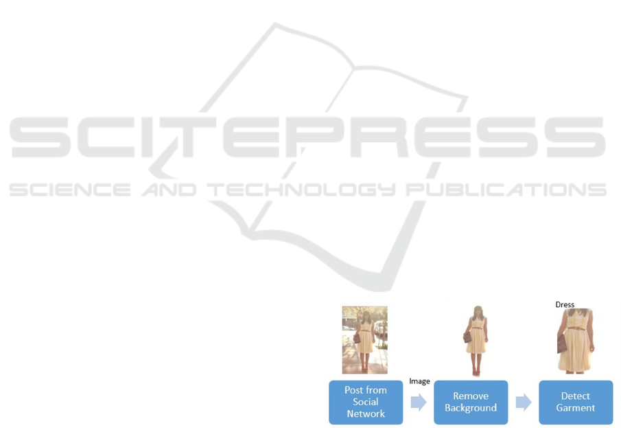
our model. Figure 2 illustrates the procedure. First,

we detect the background using U2-Net (Qin et al.,

2020) and remove it from each Instagram image, to

avoid the undesirable possibility that our model uses

the background to predict whether an outfit is

fashionable. According to an experiment with a

dataset of 16,409 dress images, removing the

background by using U2-Net can reduce the score

prediction error rate by 5.63%. Afterward, a garment

detector that uses YOLOv5 (Jocher et al., 2022)

identifies the regions in the images that contain the

garment and states its type. Thus, the irrelevant

objects and details that may affect the feature

extraction can be removed from the images. Finally,

the regions are resized appropriately to fit in our

feature extraction model, similar to the images from

Amazon.

Figure 2: An illustration of image pre-processing.

To attain a fair comparison, we train a separate

model for each garment type. The data from Amazon

are filtered based on the category of the items, which

is mostly accurate. By contrast, the images from

Instagram are filtered using the label assigned by the

detector, given that the users are not required to tag

Popularity Prediction for New and Unannounced Fashion Design Images

733

their clothes in their descriptions. 80% of the data is

used for training and the rest is for testing.

5.1.4 Evaluation Metrics

To evaluate and compare the performance of our

models, we measure the difference between the

estimated and actual scores using the mean-squared

error (MSE) metric, which has been commonly used

in related studies (e.g. Lo et al. (2019)).

Mathematically speaking, for an input image set 𝒥,

we evaluate the model based on quantity:

𝑀𝑆𝐸𝒥=

𝒥



𝑠



−𝑠





∈

𝒥

(9)

5.2 Choosing Regression Models and

Parameters

Experiments are carried out to choose the appropriate

regression methods and parameters. Table 2

summarizes the performance of using different

regression methods. While kNN has a lower mean

squared error when using the training dataset, its error

for the testing set is higher than those of Stochastic

Gradient Descent (SGD) and MLP. Passive

aggressive regression shows the worst performance

for all trials. In terms of errors, the differences

between SGD and MLP are small, but we choose the

latter because of its more options for tuning the

model.

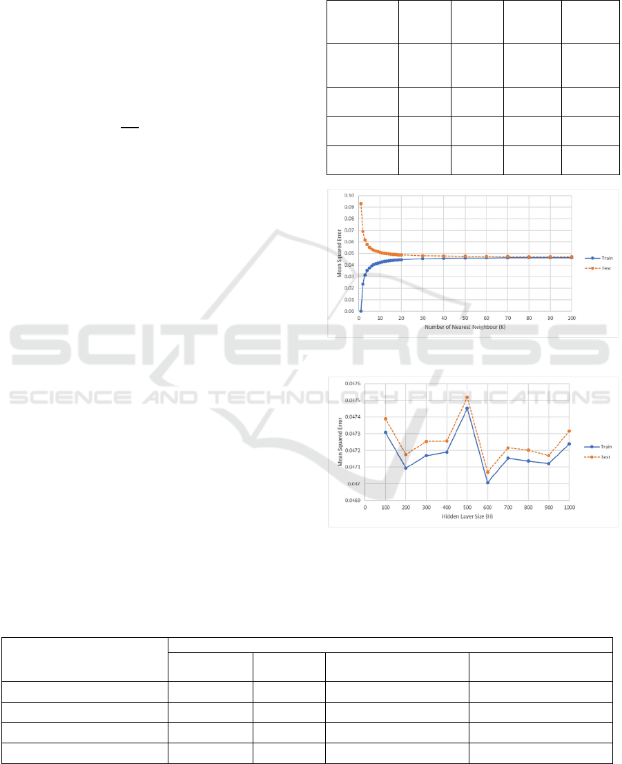
We also test different values of the nearest

neighbors to consider (K) when kNN regression is

used, and of the hidden layer size (H) when MLP

regression is used. The results of these experiments

are shown in Figure 3 and Figure

, respectively.

As K increases, the error in the testing set

decreases as that of the training set increases.

However, by increasing K, the prediction results tend

to have less deviation, an undesirable effect as the

small differences between items can cause difficulties

in interpreting their popularity. This result also

suggests that the kNN model may be over-fitted.

As for H, no general trend is observed with its

changes, but the error is highest at H = 500 and lowest

at H = 600.

Table 2: Comparison of different regression methods.

Regression

Model

Train

MSE

(

Dress

)

Test

MSE

(

Dress

)

Train

MSE

(

Blouse

)

Test

MSE

(

Blouse

)

Stochastic

Gradient

Descent

0.0471 0.0472 0.0549 0.0552

Passive

ressive

0.0530 0.0533 0.0758 0.0782

kNN

(

= 20)

0.0446 0.0487 0.0518 0.0579

MLP

(

= 600

)

0.0469 0.0471 0.0549 0.0556

Figure 3: MSE against the number of nearest neighbours.

Figure 4: MSE against hidden layer size.

Table 3: MSE of models for datasets for dresses.

Models Datasets for Dresses

Amazon Instagram Amazon and Instagram

(

without Shiftin

Amazon and Instagram

(

with Shiftin

Inception v3 only (baseline) 0.0639 0.0679 0.0785 0.0608

Inception v3 + LSTM (L = 8) 0.0401 0.0692 0.0782 0.0516

Inceptionv3 + kNN (K = 20) 0.0581 0.0704 0.0800 0.0487

Inceptionv3 + MLP (H = 600 0.0543 0.0668 0.0765 0.0471

ICAART 2023 - 15th International Conference on Agents and Artiﬁcial Intelligence

734

Table 4: MSE of models for datasets for blouses.

Models Datasets for Blouses

Amazon Instagram Amazon and Instagram

(without Shifting)

Amazon and Instagram

(with Shifting)

Ince

tionv3 onl

(

baseline

)

0.0783 0.0666 0.0791 0.0559

Ince

tionv3 + LSTM

(

= 8

)

0.0471 0.0632 0.0732 0.0556

Inceptionv3 + kNN (

= 20) 0.0541 0.0686 0.0771 0.0577

Inceptionv3 + MLP (

= 600 0.0532 0.0656 0.0752 0.0556

5.3 Performance Comparison

In this study, we compare three models to that

considered by the MLP regression. The first model,

which we refer to as the baseline, uses a modified

Inception v3 model, to predict the score. It is an end-

to-end CNN model, in which we replace its original

final layer, which is a fully connected network, with

one that contains only one neuron. The second model

is an Inception-Long Short-Term Memory (LSTM)

architecture similar to that of Lo et al. (2019). Given

that our models are designed for a specific garment

type, the garment type tag as a “textual” feature is

redundant and therefore discarded. However, the

model outputs depend on the input of previous trends

and thus may vary when the popularity scores of

different images are provided. The reason is that the

lack of a strict requirement on which image must be

fed as long as the sequence is chronological. Notably,

in our experiments, the feature extraction and the

LSTM modules are back-propagated. We set the

length of sequence L to 8, as suggested by Lo et al.

(2019). The third model used is the kNN regression

model, which compares the Euclidean distance of the

input and the known feature vectors and returns the

mean of the associated scores of the closest

neighbors.

Table 3 and Table 4 report the mean square errors

while using the consolidated datasets for dresses and

blouses respectively. MLP regression consistently

outperforms the baseline and kNN regression.

Although the LSTM model performs better in general

with its more complicated network architecture and

more input, MLP regression provides a more accurate

prediction when the dress datasets include the images

from Instagram.

We also attempt to combine the Instagram dataset

without aligning the mean and standard deviation, or

formally, setting 𝑆



= 𝑆





. The results show that

the performances of the models are better with the

alignment. By aligning the distribution of the

Instagram dataset, the MSE for all our models

decreases by approximately 25% compared with the

unaligned ones. The difference in popularity score

distribution might cause difficulties in providing

consistent results.

5.4 Challenging Cases

Predicting the popularity solely by image remains to

be a challenge, given the relevance to other factors

that are irrelevant to the appearance of the image

itself. As pointed out by Simo-Serra et al. (2015), one

of the more useful factors for predicting popularity is

the follower count of the poster. This measure may

suggest that the popularity score can highly differ

depending on the poster, even when the posts contain

identical images.

Another difficulty lies in the behavior of sellers on

e-commerce platforms. In the Amazon dataset,

several types of clothes may be listed repeatedly but

in different sizes or colors. Due to technical

constraints on Amazon, these clothes are regarded as

different items and thus have different popularity

indexes. For example, for the same image of three

maxi dress items with different sizes, the sales ranks

are 478,580 for Large, 484,586 for Medium, and

1,823,102 for Small. The regression helps predict the

popularity of the dress image by averaging, but we

cannot separately and reliably predict the popularity

of the three sizes unless more information is known,

such as the item title.

6 CONCLUSIONS

This study provides a comprehensive measurement of

the popularity of a fashion item by considering not

only its presence on social media platforms but also

its sales in e-commerce. With such metrics, we have

developed a model capable of predicting the

popularity of a clothing item through its image. Using

the output score of the model, the popularity of

different items can be compared intuitively given the

numerical result.

The eased input requirements make this model

suitable for estimating the popularity of a draft design

for fashion designers, without the need of evaluating

Popularity Prediction for New and Unannounced Fashion Design Images

735

the responses from social media platforms (which can

lead to design copies) or comparing with a large

quantity of other items (which is computationally

inefficient and raises fairness issues). This model can

help fashion designers and practitioners identify

popular fashion products in the market and more

effectively plan their production.

While this model has a rather simple input that

facilitates ease of use, this advantage comes with the

cost of reduced sensitivity to the text describing the

product. To address such limitation, we can

incorporate sentiment analysis on the review

comments on the garment items. Therefore,

combining image and text analysis can point to a

future research direction for fashion popularity

prediction.

ACKNOWLEDGEMENTS

The authors are grateful for the constructive

comments of the referees on an earlier version of this

article. This research was supported in part by

Innovation and Technology Commission, HKSAR

under grant number ZR2J.

REFERENCES

Jocher, G., Chaurasia, A., Stoken, A., Borovec, J.,

NanoCode012, Kwon, Y., et al. (2022). YOLOv5

classification models, Apple M1, reproducibility,

ClearML and Deci.ai integrations. Retrieved from

https://doi.org/10.5281/zenodo.7002879.

Kang, W.-C., Fang, C., Wang, Z., & McAuley, J. (2017).

Visually-aware fashion recommendation and design

with generative image models. In 2017 IEEE

International Conference on Data Mining (ICDM).

Kim, S., Jiang, J. Y., Nakada, M., Han, J., & Wang, W.

(2020). Multimodal post attentive profiling for

influencer marketing. In The Web Conference.

Lo, L., Liu, C. L., Lin, R. A., Wu, B., Shuai, H., H., &

Cheng, W. H. (2019). Dressing for attention: Outfit

based fashion popularity prediction. In IEEE

International Conference on Image Processing (ICIP)

McAuley, J., Targett, C., Shi, Q., & van den Hengel, A.

(2015). Image-based recommendations on styles and

substitutes. In 38th International ACM SIGIR

Conference on Research and Development in

Information Retrieval.

Qin, X., Zhang, Z., Huang, C., Dehghan, M., Zaiane, O. R.,

& Jagersand, M. (2020). U2-Net: Going deeper with

nested U-structure for salient object detection. Pattern

recognition, 106.

Simo-Serra, E., Fidler, S., Moreno-Noguer, F., & Urtasun,

R. (2015). Neuroaesthetics in fashion: Modeling the

perception of fashionability. In IEEE Conference on

Computer Vision and Pattern Recognition.

Szegedy, C., Vanhoucke, V., Ioffe, S., Shlens, J., & Wojna,

Z. (2016). Rethinking the inception architecture for

computer vision. In IEEE Conference on Computer

Vision and Pattern Recognition.

Wang, J., Nabi, A. A., Wang, G., Wan, C., & Ng, T.-T.

(2015). Towards predicting the likeability of fashion

images. arXiv preprint arXiv:1511.05296.

Xiao, H., Rasul, K., & Vollgraf, R. (2017). Fashion-mnist:

a novel image dataset for benchmarking machine

learning algorithms. arXiv preprint arXiv:1708.07747.

Zhang, Y., & Caverlee, J. (2019). Instagrammers,

fashionistas, and me: Recurrent fashion

recommendation with implicit visual influence. In 28th

ACM International Conference on Information and

Knowledge Management (CIKM '19).

ICAART 2023 - 15th International Conference on Agents and Artiﬁcial Intelligence

736