Wearable Data Generation Using Time-Series Generative Adversarial

Networks for Hydration Monitoring

Farida Sabry

1 a

, Wadha Labda

1 b

, Tamer Eltaras

1 c

, Fatima Hamza

1 d

, Khawla Alzoubi

2 e

and Qutaibah Malluhi

1 f

Qatar University, Doha, Qatar

Engineering Technology Department, Community College of Qatar, Doha, Qatar

Keywords:

Data Generation, Synthetic Data, GAN, Wearable Devices, Biosignals.

Abstract:

Collection of biosignals data from wearable devices for machine learning tasks can sometimes be expensive

and time-consuming and may violate privacy policies and regulations. Successful and accurate generation

of these signals can help in many wearable devices applications as well as overcoming the privacy concerns

accompanied with healthcare data. Generative adversarial networks (GANs) have been used successfully in

generating images in data-limited situations. Using GANs for generating other types of data has been actively

researched in the last few years. In this paper, we investigate the possibility of using a time-series GAN

(TimeGAN) to generate wearable devices data for a hydration monitoring task to predict the last drinking

time of a user. Challenges encountered in the case of biosignals generation and state-of-the-art methods for

evaluation of the generated signals are discussed. Results have shown the applicability of using TimeGAN

for this task based on quantitative and visual qualitative metrics. Limitations on the quality of the generated

signals were highlighted with suggesting ways for improvement.

1 INTRODUCTION

The recent advances in wearable technology have mo-

tivated researchers and industry to investigate many

machine learning based applications that can learn

from the vast amount of signals from wearable sen-

sors (Sabry et al., 2022a). There are a variety of non-

invasive signals that can be captured from the human

body using different sensors to learn about the health

condition of the user for a wide variety of machine

learning healthcare applications (Sabry et al., 2022a).

Some of the problems that arise with these types of

applications are the cost and time associated with the

data collection phase, the limited size of datasets used

for training (Sabry et al., 2022b; Delmastro et al.,

2020). Additionally, the collection of biosignals data

is erroneous which increases the cost and time even

more. Data collection of health data is subjected to

https://orcid.org/0000-0001-5639-983X

https://orcid.org/0000-0001-6097-2395

https://orcid.org/0000-0002-8664-9091

https://orcid.org/0000-0002-3689-7003

https://orcid.org/0000-0002-2797-2673

https://orcid.org/0000-0003-2849-0569

many regulations to ensure the safety of subjects and

preserve the privacy of their sensitive data. Though

anonymizing this sensitive data by removing identi-

fying features or adding noise and grouping individu-

als into broader categories is sometimes done to over-

come this privacy problem, it is usually not effective

with small dataset sizes used in research from wear-

able devices.

One way to overcome these problems is to gener-

ate synthetic training data that follows the same dis-

tribution for real world data (Piacentino et al., 2021;

Zhou et al., 2019; Yoon et al., 2019). Synthetic data

can be used with various objectives such as data un-

derstanding, data imputation (Luo et al., 2018), data

correction and noise removal (Kiranyaz et al., 2022;

Lu et al., 2021; Zargari et al., 2021), data augmenta-

tion (Um et al., 2017; Kiyasseh et al., 2020; Lo et al.,

2021; Montero et al., 2021), and data privacy (Xin

et al., 2020; Nguyen et al., 2020; Piacentino et al.,

2021).

A synthetically generated dataset must have the

same mathematical and statistical properties as the

real-world dataset. For biosignals generation, there

are additional constraints on the shape and repeated

pattern of some signals which must be preserved in

Sabry, F., Labda, W., Eltaras, T., Hamza, F., Alzoubi, K. and Malluhi, Q.

Wearable Data Generation Using Time-Series Generative Adversarial Networks for Hydration Monitoring.

DOI: 10.5220/0011757200003414

In Proceedings of the 16th Inter national Joint Conference on Biomedical Engineering Systems and Technologies (BIOSTEC 2023) - Volume 4: BIOSIGNALS, pages 94-105

ISBN: 978-989-758-631-6; ISSN: 2184-4305

 2023 by SCITEPRESS – Science and Technology Publications, Lda. Under CC license (CC BY-NC-ND 4.0)

synthetic data. The generated data has to be realis-

tic enough to gain true insights from it when used in

different machine learning tasks (Sabry et al., 2022a).

Synthetic data is less subjected to data privacy con-

cerns or missing values problems. Synthetic data gen-

eration has been approached using many techniques

that either change the real data to guarantee its pri-

vacy such as differential privacy (Ping et al., 2017;

Xin et al., 2020; Um et al., 2017) or learn from the

real data using a variety of machine-learning tech-

niques (Reiter, 2005; Zhang et al., 2017; Xu et al.,

2019; Yoon et al., 2019) to learn the distribution of

the data and then sample the distribution to generate

the synthetic data.

Generative adversarial networks (GANs) are

among the machine learning techniques that can be

used to generate synthetic data that is similar to the

actual data in terms of data distribution and statisti-

cal features. The authors in (Goodfellow et al., 2014)

were the ﬁrst to introduce GAN to generate new syn-

thetic image data that are difﬁcult to be distinguished

from real data images but at the same time not memo-

rized from the training set. With the potential of GAN

and development of research for its variants, GAN has

been used to generate various other types of data such

as tabular data with discrete and continuous values

(Xu et al., 2019). Although there are some similar-

ities in the used techniques, there are differences in

implementation for every type of data which requires

some adjustments in the GAN architecture. In this

study, we investigate the use of a variant of GAN, spe-

ciﬁc for time-series data (Yoon et al., 2019), to gener-

ate synthetic data of different biosignals which have

special characteristics such as amplitude thresholds,

repetitive pattern, positions of peaks and troughs to

be used for hydration monitoring based on the real

dataset we collected in (Sabry et al., 2022b). Though

there are some studies (Furdui et al., 2021; Belo et al.,

2017; Zhou et al., 2019) that used other types of

GANs to generate electrocardiogram (ECG) or gal-

vanic skin response (GSR) signals for other classiﬁ-

cation tasks, but few studied using GANs for a regres-

sion problem (Ning et al., 2018) and for the best of our

knowledge this is the ﬁrst study to use GAN for hy-

dration monitoring data generation to predict the last

drinking time.

The rest of the paper is organized as follows. Sec-

tion 2 reviews brieﬂy the background for this re-

search giving a summarized overview for GAN and

its variants. Related work for using GANs for biosig-

nals generation and challenges for biosignals data are

discussed in this section as well. Section 3 brieﬂy

describes the dataset (Sabry et al., 2022b) used in

this research. In section 4, the methodology for us-

ing times-series GAN for synthetic data generation

for hydration monitoring is presented, together with

the used evaluation metrics. Results and discussion

are presented in section 5. The paper is then con-

cluded in section 6 with a summary of the research,

its results, its limitations and future improvements are

highlighted.

2 BACKGROUND AND RELATED

WORK

Generative adversary network (GAN) is a machine

learning model that is simply based on two deep neu-

ral networks; one is called the generator network (G)

and the other is called discriminator network (D) and

both of them compete in a zero-sum game to reach

Nash equilibrium with a value function V (D, G) given

in Equation 1 where x represents the input real sam-

ples to the discriminator and z represents the input

noise samples to the generator from which it starts

to generate fake data G(z). While G works on gener-

ating realistic data by minimizing V, D is a classiﬁer

that is used to differentiate the real and fake data as

genuinely as possible by maximizing V . A typical

GAN model is shown in Figure 1, both the generator

and discriminator typically have multiple convolution

layers to capture the details of the input data. GAN

was ﬁrst introduced by Goodfellow et al (Goodfellow

et al., 2014) in 2014 and since then research has been

developing different GAN variants that were able to

generate images, videos, music notes, etc with high

quality. The authors in (Jabbar et al., 2022) review the

different variants of GANs, their wide range of appli-

cations, shortcomings affecting the training stability

and different training solutions.

min

max

V (D, G) =

x∼p

data

(x)



logD (x)



z∼p

(z)



log (1 − D (G(z)))



(1)

The basics for generative modeling in GAN can be

seen as improvements to autoencoders. Autoencoder

and its probabilistic version, variational autoencoder,

are used to represent high-dimensionality data and

compress it into a small representation with simple

neural networks (encoder and decoder) without mas-

sive data loss (Jabbar et al., 2022). Generative models

were then used to to improve the quality of the gener-

ated data and guarantee better privacy protection mea-

sures. Here we list some examples for GAN variants

used in literature for generation of different biosignals

which have special characteristics and challenges dif-

Wearable Data Generation Using Time-Series Generative Adversarial Networks for Hydration Monitoring

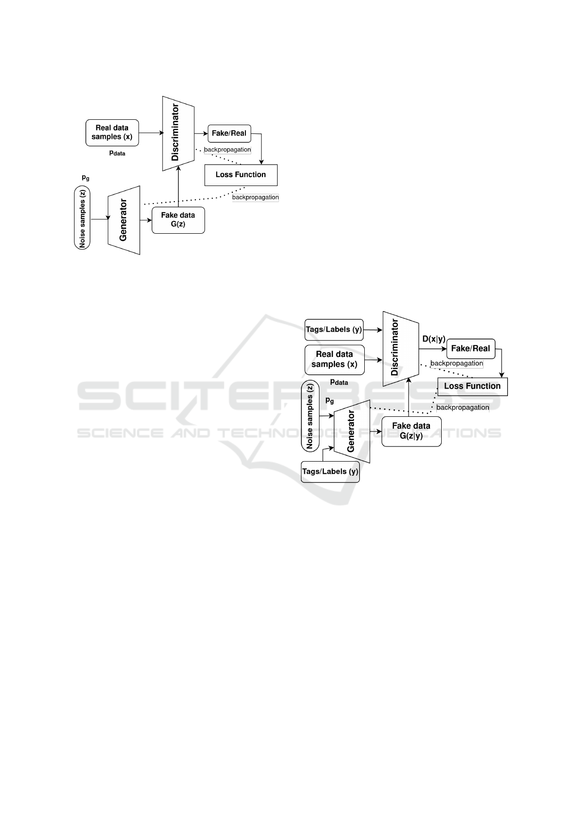
Figure 1: General GAN architecture.

ferent from images that will be discussed in the next

subsection.

• Conditional GAN: It is very similar to the sim-

ple GAN in Figure 1 but with the output of the

generator and discriminator conditioning on la-

bels y or any additional information in general for

both the real samples and the noise samples as

shown in Figure 2 with modiﬁed objective func-

tion in Equation 2 to improve the diversity of the

generated dataset. The ﬁrst term in the objec-

tive function is the expected log likelihood of the

real data samples under the discriminator, given

the label or context y that the discriminator is

trying to predict. The second term is the ex-

pected log likelihood of the synthetic data sam-

ples under the discriminator, given the label or

context y. It has been used in (Kiyasseh et al.,

2020) for the generation of pathological photo-

plethysmogram (PPG) signals in order to boost

medical classiﬁcation performance for different

cardiac classes. PPG signals were downsampled

and split into overlapping 5sec-frames and fed to

three different CGANs which may not handle the

temporal behavior of the data and produce un-

realistic data. They modiﬁed the loss functions

with different terms to improve inter-class diver-

sity and penalize the network for generating unre-

alistic samples. In (Harada et al., 2018), they pro-

posed forming each neural network in GAN based

on a recurrent neural network (RNN) using long

short-term memories (LSTM) for its hidden lay-

ers to deal with the time-series data generation for

ECG and EEG signals. An ICU dataset record-

ing oxygen saturation, heart rate, respiratory rate

and mean arterial pressure has been used in (Es-

teban et al., 2017) to generate synthetic data for

various ICU prediction tasks of whether a patient

will go in a critical condition deﬁned by thresh-

olds for these variables. They showed that the

prediction accuracy decreases when training with

synthetic data by a maximum of 12%. Generating

synthetic signals for four kinds of biomedical sig-

nals (electrocardiogram (ECG), electroencephalo-

gram (EEG), electromyography (EMG), photo-

plethysmography (PPG)) was done in (Hazra and

Byun, 2020). They used a CGAN with bidirec-

tional grid long short-term memory for the gener-

ator network and convolutional neural network for

the discriminator network to capture time-series

dependency.

min

max

V (D, G) =

x∼p

data

(x)



logD (x|y)



z∼p

(z)



log (1 − D (G(z|y)))



(2)

Figure 2: Conditional GAN architecture.

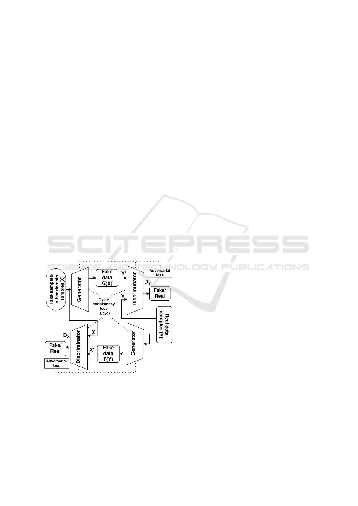
• Cycle GAN (Zhu et al., 2017): It is a special kind

of conditional GAN where the condition is not a

label or tag but rather a sample data from a dif-

ferent domain, in the case of data generation it

can be mapping of a sample from synthetic data

to real data or vice versa, one GAN works in the

forward cycle and the other in the backward, or

it can be to transform one raw signal to a de-

rived signal. General architecture for a cycle GAN

can be modeled as shown in Figure 3 and its full

objective function is given in Equation 3 where

adversarial losses for the forward and backward

GANs are calculated as in Equation 1 and L

cyc

calculated according to Equation 4 to ensure cy-

cle consistency by reducing the possibilities for

the mapping function so that an individual input

can be mapped to a desired output y

. How-

ever, cycle GANs require a relatively big dataset

BIOSIGNALS 2023 - 16th International Conference on Bio-inspired Systems and Signal Processing

to reduce the replication percentage of the gener-

ated data. For biosignals generation, Cycle GAN

has been used in (Aqajari et al., 2021) for respi-

ratory rate estimation through learning a mapping

of PPG signals to respiratory signals and updat-

ing the objective function to include a weighted

term that takes into account the respiratory rate of

the generated respiratory signals. It has been used

in (Zargari et al., 2021) too, for noise artifacts re-

moval without depending on accelerometer data

through PPG signal to image transformation. The

authors in (Kiranyaz et al., 2022) also used oper-

ational cycle-GANs for ECG signals restoration,

not whole signal generation. They used quanti-

tative evaluation by measuring the performance

gain for peak detection as well as the visual qual-

itative evaluation.

L (G, F, D

, D

) = L

GAN

(G, D

, X, Y )+

GAN

(F, D

, Y, X )+

λL

cyc

(G, F)

(3)

cyc

(G, F) =

x∼p

data

(x)



∥(F (G (x))) − x∥



y∼p

data

(y)



∥(G(F (y))) − y∥



(4)

Figure 3: Cycle GAN architecture.

• Wasserstein GAN (W-GAN) (Arjovsky et al.,

2017): It is very similar to the traditional GAN

but with calculating the loss function based on

Wasserstein distance between the real data distri-

bution and the generated data distribution rather

than depending on Jensen–Shannon divergence.

This GAN variant was introduced to solve mode

collapse problem which is a GAN training chal-

lenge. In the context of biosignal generation, an

auxiliary conditioned WGAN has been used in

(Furdui et al., 2021) to generate galvanic skin re-

sponse (GSR) and electocardiogram (ECG) sig-

nals that can be used for arousal classiﬁcation by

combining the Wasserstein loss with the gradi-

ent penalty and classiﬁcation loss to discard sig-

nals that doesn’t improve the classiﬁcation to en-

hance the generalizability of emotion recognition

algorithms. WGAN was also used with modiﬁed

Gate Recurrent Units (GRUs) in (Luo et al., 2018)

for imputation of data in physionet dataset, au-

thors were able to model the temporal irregularity

of the incomplete time series. Their results out-

performed the baselines in terms of accuracy of

imputation for the missing data during recording

process.

• Style Generator Architecture for GAN (Style

GAN): It is a modiﬁed architecture to GAN where

more complexity is added to the generator to have

26.2M trainable parameters (Karras et al., 2021).

This is done through adding a mapping network of

fully connected layers to map the input to a latent

representation, followed by a synthesis network

which is controlled by this representation through

adaptive instance normalization (AdaIN) at each

convolution layer. This aims to achieve better in-

terpolation and also model the factors of variation

better, its usage has vastly improved the gener-

ation of images that feel-like real. A variant of

style GAN was used in (Montero et al., 2021) for

fetal brain ultrasound plane classiﬁcation. It was

used in (Thambawita et al., 2021) for generation

of gastroenterology data images. To the best of

our knowledge, styleGAN hasn’t been applied to

biosignals with time-series patterns.

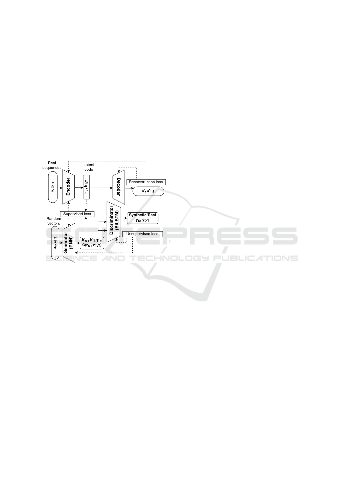
• Time-series GAN (Yoon et al., 2019) is another

type of GAN that combines the traditional un-

supervised GAN network with a supervised au-

toregressive model to model the temporal dynam-

ics of a time-series. A typical architecture of the

TimeGAN is shown in Figure 4. Weights are up-

dated based on three losses; the supervised loss,

the unsupervised loss and the reconstruction loss

of the autoregressive model deﬁned as in Equa-

tions 5, 6 and 7 respectively where the expected

log likelihood is calculated over all time steps for

both real and synthetic data. It has been used to

generate stock and energy prediction data and re-

ported improvement over other CGANs with units

that capture temporal dynamics such as RNN and

LSTM (Brophy et al., 2021). It hasn’t been ap-

plied before for biosignals data generation as we

Wearable Data Generation Using Time-Series Generative Adversarial Networks for Hydration Monitoring

propose in this paper.

supervised

s,x

1:T

∼p



∑

∥h

− G

, h

t−1

, z

)∥



(5)

unsupervised

s,x

1:T

∼p



log(y

) +

∑

log(y

)



s,x

1:T

∼p

′



log(1 − y

′

) +

∑

log(1 − y

′

)



(6)

reconstruction

s,x

1:T

∼p



∥s − s

′

∥

∑

∥x

− x

′

∥



(7)

Figure 4: Time-series GAN architecture.

2.1 Challenges of Biosignals Generation

Biosignals dataset collection is considered very chal-

lenging for many reasons. Most of the time, the real

dataset is with a limited number of subjects due to

the cost involved and the privacy constraints. The

collected data may suffer from missing/incorrect data

due to errors in sensors’ attachment or noisy sig-

nals due to motion artifacts (Elgendi, 2016). There

are other inadequacies that might appear in the col-

lected data which include insufﬁcient measurement

time, different sensors’ conﬁgurations used by dif-

ferent subjects and inconsistent measurement times

(Hernang

omez et al., 2022). Generative modeling to

generate synthetic data based on the real biosignals

dataset collected consequently becomes challenging.

In addition to the paucity of the collected data and

its aforementioned inadequacies, class imbalance data

(Kiyasseh et al., 2020) for infected or abnormal sam-

ples pose other difﬁculties for synthetic data genera-

tion.

Real-world tabular data collected for biosignals

usually consists of mixed types; continuous data for

signals from sensors such as photoplethysmography

(PPG), ECG, GSR, accelerometer, magnetometer, gy-

roscope and discrete data such as sex, age, medicine

intake, etc. To generate a mix of these discrete and

continuous data simultaneously, GANs must apply

both softmax and tanh on the output (Xu et al., 2019).

Modeling this kind of mixed tabular data in general

to generate realistic data is a non-trivial task (Xu

et al., 2019). A review for some approaches to han-

dle discrete data is presented in (Jabbar et al., 2022).

Continuous data for biosignals usually follow a non-

Gaussian distribution unlike the images pixel values

which follow a Gaussian-like distribution. In GANs,

the last layer has a tanh function which can success-

fully output a value in the range [-1,1] for images data

after normalization using a min-max transformation

whereas continuous non-Gaussian data will lead to

vanishing gradient problem.

As well known in the machine learning ﬁeld,

highly imbalanced data poses many challenges for

learning in general and for learning a GAN model

in particular as minority classes are underrepresented

making a GAN susceptible to severe mode collapse.

In this case, the generator produce outputs with small

diversity leading to only slight changes to the data dis-

tribution that may be hardly detected by the discrim-

inator. To decrease this effect and prevent the gener-

ator from optimizing for a single ﬁxed discriminator,

Wasserstein loss is used to avoid the discriminator be-

ing stuck in local minima. Unrolled GAN (Metz et al.,

2017) is another way to face this problem which uses

a generator loss function based on the current and fu-

ture discriminator’s classiﬁcations so that the genera-

tor don’t optimize for a single discriminator.

In the next subsection, we review the sate-of-art

evaluation metrics to evaluate GANs.

2.2 Evaluation Metrics

Evaluation of GAN models is an active research area

regarding unstable training (Jabbar et al., 2022) as

there is no standard function for evaluation. In this

section, we brieﬂy review the different evaluation

metrics used in literature to evaluate the GAN and

outputs generated by it.

Evaluation metrics can be classiﬁed as qualitative

or quantitative. Qualitative evaluation refers to human

visual assessment for the generated samples from the

GAN but it lacks a suitable objective evaluation met-

ric. Quantitative evaluation refers to objective metrics

that either assess the similarity of the generated syn-

thetic data to the real data, calculate the distance be-

BIOSIGNALS 2023 - 16th International Conference on Bio-inspired Systems and Signal Processing

tween the two distributions or evaluate the accuracy

for the classiﬁcation task or regression error when

replacing the real dataset with synthetic dataset for

training the machine learning model. Most of the pro-

posed metrics in literature are applicable to the image

data (Brophy et al., 2021).

For image data, inception-score (IS) and Fr

echet

inception distance (FID) are most commonly used to

evaluate the diversity and quality of the generated

samples for its correlation with human ﬁndings of the

generated samples (Jabbar et al., 2022).

Pearson correlation coefﬁcient was used in (Hazra

and Byun, 2020) to verify the quality of synthetic

data when compared to the original data as well as

root mean square error (RMSE), percent root mean

square difference (PRD), mean absolute error (MAE),

and Frechet distance (FD) for statistical analysis.

However, they were used as one-to-one measure be-

tween synthetic data and original data used to gener-

ate it with assumption of having the same sequence

length as the original data (aligned sequences of ﬁxed

length).

Propensity score which represents the probabil-

ities of whether a record is real or synthetic, has

been used for many record data (Dankar and Ibrahim,

2021). It involves building a binary classiﬁcation

model for classiﬁcation but not formulated for time-

series data. To deal with time-series data, authors in

(Yoon et al., 2019) introduced a discriminative score

as a quantitative measure for similarity using a 2-

layer LSTM to classify sequences as either synthetic

or original. The classiﬁcation error is the score and

the less error means the generated sequences are simi-

lar to the original data. They also introduced a predic-

tive score which is similar to the Train on Synthetic,

Test on Real where a sequence-prediction model with

2-layer LSTM is trained to predict next-step tem-

poral vectors over each input sequence. Then, the

trained model is tested on the original dataset. For

visualizing how closely the distribution of generated

data represents that of the original, authors in (Yoon

et al., 2019) used t-Stochastic Neighbor Embedding

(t-SNE) (van der Maaten and Hinton, 2008) and prin-

cipal component analysis (PCA) (Bryant and Yarnold,

2001) by ﬂattening the temporal dimension on both

the original and synthetic datasets and results are as-

sessed visually.

As can be deduced from the above brief review,

there are no standard evaluation metric for fair model-

to-model comparison and specially when it comes

to time-series data. The development of a quantita-

tive evaluation metric for the synthetic data genera-

tion still requires future research, especially for time-

series data. As this is not the main focus of the pa-

per, we chose to use the scores used by (Yoon et al.,

2019) as they are the only ones developed for time

sequences. Additionally, we used Train on Synthetic

Test on Real (TSTR) metric as this is the main goal

for the generation of synthetic data to use more data

for learning a model that can predict the output value

in the regression problem of hydration monitoring for

the last drinking time.

3 DATASET

For generating wearable device data for the task of

hydration monitoring, we used the real dataset we col-

lected in (Sabry et al., 2022b) using sensors from the

calibrated Shimmer Galvanic Skin Response (GSR)

unit

. The last time for water and food intake was

recorded for subjects wearing the GSR unit who

fasted during Ramadan or were voluntary fasting with

no restrictions on movement or the time of wear-

ing the device and also in non-fasting conditions, i.e.

the last drinking time is within 1 hour. The signals

are recorded from the shimmer device at a frequency

of 512 Hz and include PPG, GSR Skin Resistance,

GSR Skin Conductance, accelerometer in the three

directions (X,Y,Z), magnetometer (X,Y,Z), gyroscope

(X,Y,Z), ambient temperature and pressure. A total of

3386 min (56.4 h) data were collected from 11 healthy

subjects (9 females and 2 males). All data collection

was subject to Qatar University Institutional Review

Board (IRB) approval procedures covered by the IRB

approval: QU-IRB 1538-EA/21. The raw dataset is

available at Zenodo

4 WEARABLE DATA

GENERATION

The approach followed for generating wearable data

that can be used for hydration monitoring task in

(Sabry et al., 2022b) can be presented as shown in

Figure 5. First, a real dataset was built of the biosig-

nals from the wearable device (PPG, GSR) as well

as that of the movement sensors (accelerometer, mag-

netometer and gyroscope) and the ambient tempera-

ture and pressure sensors as discussed in the previous

section. Preprocessing of the dataset included down-

sampling the signals at 1 min intervals and extract-

ing features from signals aggregating the mean val-

http://www.shimmersensing.com/products/gsr-optical

-pulse-development-kit (accessed on 16 Nov. 2022)

https://zenodo.org/record/6299964 (accessed on 16

Nov. 2022)

Wearable Data Generation Using Time-Series Generative Adversarial Networks for Hydration Monitoring

ues and calculating the accumulated changes in the

magnitude for accelerometer, magnetometer and gy-

roscope data (Sabry et al., 2022b) as in Equations

8, 9, 10, 11, 12 and 13. |ACC| refers to the mag-

nitude of the accelerometer from the components in

the three directions (acc

, acc

). cumAcc is

the accumulative change in accelerometer magnitude

over time. |MAG| refers to the magnitude of the

magnetometer from the components in the three di-

rections (mag

, mag

). cumMag is the ac-

cumulative change in magnetometer magnitude over

time. |GY RO| refers to the magnitude of the gyro-

scope from the components in the three directions

(gyro

, gyro

). cumGyro is the accumulative

change in gyroscope magnitude over time. These

magnitude values for accelerometer, magnetometer

and gyroscope as well as the accumulative changes

in them that represent the motion jerk can reﬂect the

effort and state of activity of the subject. For the hy-

dration monitoring task, the ﬁne details of the signals

is not as relevant as the big changes of it through

time so downsampling and aggregation can be seen

feasible. It also helps in speeding up the training of

the generative adversary network for time-series data

(TimeGAN).

The output signals together with the column for

the recorded last drinking time for each of the fasting

and non-fasting samples for each subject are then in-

put to the TimeGAN module and are considered the

real sequences. The TimeGAN generator uses gated

recurrent units in its recurrent neural network with 20

hidden nodes in each of its three layers and the dis-

criminator uses bidirectional long short-term memory

units to increase the amount of information available

to the network. The generated synthetic signals are

then updated with the objective to minimize the three

loss functions in Equations 5, 6 and 7 for 500 iter-

ations. The TimeGAN is then evaluated using dis-

criminative score (Yoon et al., 2019) mentioned in

section 2.2 with lower value means better. It repre-

sents the post-hoc classiﬁcation error for a supervised

classiﬁer fed with original signals labeled as real ex-

amples and generated signals labeled as synthetic ex-

amples and tested with a held-out test set. A predic-

tive score is also calculated to evaluate the effective-

ness of TimeGAN to capture the conditional distribu-

tions over time. It represents the mean absolute error

(MAE) in predicting the next-step temporal vectors

over each input sequence in the original dataset using

an LSTM model trained with the synthetic generated

dataset.

Training on synthetic data and testing on real was

done for the main problem of hydration monitoring

where we trained the three models that achieved the

Table 1: Mean discriminative and predictive scores for gen-

erated fasting and non-fasting data.

Discriminative score Predictive score

fasting 0.319 3.9

non-fasting 0.225 0.276

best performance in (Sabry et al., 2022b); random for-

est, gradient boosted regression and extra trees.

|ACC| =

(acc

+ acc

) (8)

cumAcc =

t−1

∑

j=1

|ACC|

j+1

− |ACC|

(9)

|MAG| =

(mag

+ mag

) (10)

cumMag =

t−1

∑

j=1

|MAG|

j+1

− |MAG|

(11)

|GY RO| =

(gyro

+ gyro

) (12)

cumGyro =

t−1

∑

j=1

|GY RO|

j+1

− |GY RO|

(13)

5 RESULTS

5.1 Quantitative Evaluation

The synthetic output of the TimeGAN is evaluated

quantitatively using the discriminative and predic-

tive scores for the output of TimeGAN obtained after

training for 500 iterations as shown in Table 1. The re-

sults show that the average predictive score for gener-

ating fasting samples is relatively high, this can be at-

tributed to the smaller number of samples and shorter

sequences used in training the TimeGAN with fasting

sequences as well as the missing of some other fea-

tures in the original dataset we used in (Sabry et al.,

2022b) such as height, weight, sex and age which af-

fect these signals differently during fasting.

The generation with different fasting and nonfast-

ing samples in the dataset from different subjects was

used to check for the relation between the discrimina-

tive and predictive scores and the length of the gen-

erated sequences. The results are shown in Figure 6

and no relation can be inferred for the dependence of

theses scores on the length of the generated sequence.

BIOSIGNALS 2023 - 16th International Conference on Bio-inspired Systems and Signal Processing

100

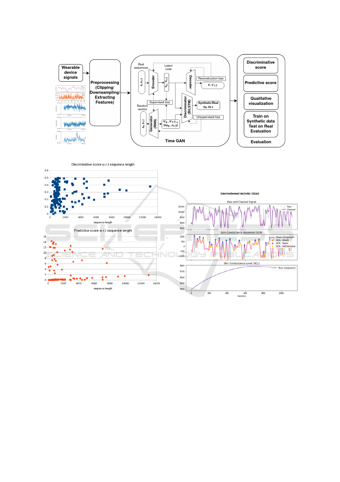
Figure 5: Overview of the wearable data generation steps.

Figure 6: Discriminative score (a) and predictive score (b)

vs generated sequence length.

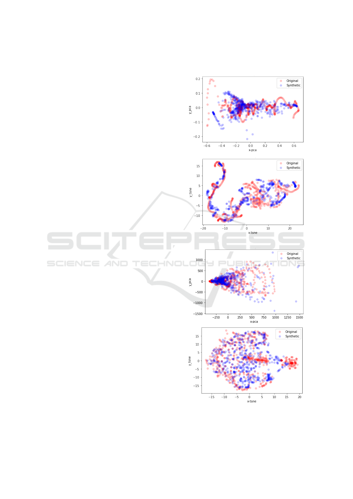
5.2 Qualitative Visualization

As for the qualitative visualization to assess how the

distribution of the generated signals is close to that of

the real signal, ﬂattening of the time-series sequence

for all signals was done using the functions provided

by the authors of (Yoon et al., 2019). PCA and t-SNE

visualizations are shown in Figure 8 for both fasting

and non-fasting sequences. The ﬁgure shows the syn-

thetic data projections are closely following that of

the original data for these groups of sequences and

the rest of sequences show similar closeness with few

exceptions. A collective quantitative metric is prefer-

ably to be introduced to evaluate the overall distance

from the original distribution for all sequences.

Plotting samples of the generated signals sepa-

rately however doesn’t show good quality signals

most of the time e.g. an electrodermal activity signal

in Figure 7 plotted from a GSR generated signal.

Figure 7: Galvanic skin response generated sample.

5.3 Training on Synthetic Test on Real

The results of the hydration monitoring task for pre-

dicting the last drinking time were evaluated by gen-

erating balanced synthetic data for fasting and non-

fasting since the original data was having more non-

fasting samples. Different synthetic data sizes were

generated and used for training the best performing

models in (Sabry et al., 2022b), namely random for-

est, gradient boosted regression and extra trees. The

average results for 10 runs are shown in Figure 9. It

can be shown in the three graphs in Figure 9 that us-

ing synthetic data has decreased the root-mean-square

error for prediction with respect to training with the

small unbalanced real dataset (TRTR) represented by

Wearable Data Generation Using Time-Series Generative Adversarial Networks for Hydration Monitoring

101

the red line on top of the graphs with a best case of

approximately 1 hour difference in the case of using

Gradient Boosted Regressor to predict the last drink-

ing time. The best RMSEs are achieved especially for

cases when the real dataset sizes used for training are

less than 1500 samples, after that the differences in

the accuracy in prediction between using generated

data and real data in training start to shrink. This

suggests the feasibility of generation of wearable data

biosignals using TimeGAN to predict the last drink-

ing time in a hydration monitoring application espe-

cially in cases of small real dataset sizes collected. As

pointed out in (Sabry et al., 2022b), predicting the last

drinking time can provide the ﬂexibility of adjusting

the alerting threshold on the wearable device based

on the health conditions, needs, and activity of the

user. The alerted user/caregiver can then choose to in-

put the correct drinking time if the prediction was not

accurate for his/her situation to enable a closed-loop

solution with online training to take place to improve

the model’s accuracy.

6 CONCLUSION

In this paper, we proposed using a generative adver-

sarial networks model, speciﬁcally designed for time-

series data, known as TimeGAN (Yoon et al., 2019)

to test its applicability for generating wearable biosig-

nals data. It was able to generate the synthetic wear-

able data signals with low discriminative and predic-

tive scores. Low discriminative score means a clas-

siﬁer can’t distinguish between original and synthetic

dataset samples. Low predictive score means that the

post-hoc sequence-prediction model is able to pre-

dict next-step temporal data signals for each input se-

quence. Visual evaluation also showed that most of

the generated signals are following the same distri-

bution of the original data. Training with synthetic

data and testing on real (TSTR) also showed that us-

ing synthetic data has decreased the root mean square

error (RMSE) for the regression task of predicting the

last drinking time compared to the training on real

testing on real (TRTR) for using different synthetic

data sizes.

One of the main objectives of biosignal wear-

able data generation is to protect the privacy of the

users’ data used in training, another evaluation met-

ric needs to be added to assess TimeGAN’s privacy

and its resistance to leak real data that participated in

the training by just the GAN memorising it (Boun-

liphone et al., 2016; Esteban et al., 2017). Another

metric for every type of synthetic biosignal generated

could be evaluated to test the quality of the generated

signals and possibly categorize them like classifying

PPG signals quality in (Elgendi, 2016).

(a) For fasting sequences.

(b) For non fasting sequences.

Figure 8: Qualitative PCA and tSNE visualization for fast-

ing and non-fasting sequences.

BIOSIGNALS 2023 - 16th International Conference on Bio-inspired Systems and Signal Processing

102

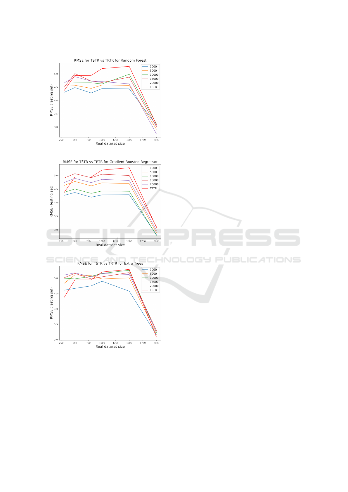
(a) Random Forest.

(b) Gradient Boosted Regressor.

Figure 9: Train Synthetic Test Real vs Train Real Test Real

for different models.

ACKNOWLEDGEMENTS

This publication was made possible by a grant from

the Qatar National Research Fund (QNRF), Project

Number ECRA 01-006-1-001. The contents of this

research are solely the responsibility of the authors

and do not necessarily represent the ofﬁcial views of

the Qatar National Research Fund (QNRF).

REFERENCES

Aqajari, S. A. H., Cao, R., Zargari, A. H. A., and

Rahmani, A. M. (2021). An End-to-End and Ac-

curate PPG-based Respiratory Rate Estimation Ap-

proach Using Cycle Generative Adversarial Net-

works. arXiv:2105.00594 [cs, eess]. arXiv:

2105.00594.

Arjovsky, M., Chintala, S., and Bottou, L. (2017). Wasser-

stein gan.

Belo, D., Rodrigues, J., and Vaz, J. (2017). Biosignals

learning and synthesis using deep neural networks.

BioMed Eng Online, 16.

Bounliphone, W., Belilovsky, E., Blaschko, M. B.,

Antonoglou, I., and Gretton, A. (2016). A test of rela-

tive similarity for model selection in generative mod-

els. In Bengio, Y. and LeCun, Y., editors, 4th Interna-

tional Conference on Learning Representations, ICLR

2016, San Juan, Puerto Rico, May 2-4, 2016, Confer-

ence Track Proceedings.

Brophy, E., Wang, Z., She, Q., and Ward, T. (2021). Gen-

erative adversarial networks in time series: A survey

and taxonomy. arXiv.

Bryant, F. and Yarnold, P. (2001). Principal-component

analysis and exploratory and conﬁrmatory factor

analysis. American Psychological Association.

Dankar, F. K. and Ibrahim, M. (2021). Fake it till you make

it: Guidelines for effective synthetic data generation.

Applied Sciences, 11(5).

Delmastro, F., Martino, F. D., and Dolciotti, C. (2020).

Cognitive Training and Stress Detection in MCI Frail

Older People Through Wearable Sensors and Machine

Learning. IEEE Access, 8:65573–65590.

Elgendi, M. (2016). Optimal signal quality index for

photoplethysmogram signals. Bioengineering (Basel,

Switzerland), 3(21).

Esteban, C., Hyland, S. L., and R

atsch, G. (2017). Real-

valued (Medical) Time Series Generation with Recur-

rent Conditional GANs.

Furdui, A., Zhang, T., Worring, M., Cesar, P., and El Ali,

A. (2021). Ac-wgan-gp: Augmenting ecg and gsr sig-

nals using conditional generative models for arousal

classiﬁcation. In Adjunct Proceedings of the 2021

ACM International Joint Conference on Pervasive and

Ubiquitous Computing and Proceedings of the 2021

ACM International Symposium on Wearable Comput-

ers, UbiComp ’21, page 21–22, New York, NY, USA.

Association for Computing Machinery.

Goodfellow, I., Pouget-Abadie, J., Mirza, M., Xu, B.,

Warde-Farley, D., Ozair, S., Courville, A., and Ben-

gio, Y. (2014). Generative adversarial nets. In Ghahra-

mani, Z., Welling, M., Cortes, C., Lawrence, N., and

Weinberger, K., editors, Advances in Neural Infor-

mation Processing Systems, volume 27. Curran Asso-

ciates, Inc.

Wearable Data Generation Using Time-Series Generative Adversarial Networks for Hydration Monitoring

103

Harada, S., Hayashi, H., and Uchida, S. (2018). Biosig-

nal data augmentation based on generative adversarial

networks. volume 2018, pages 368–371.

Hazra, D. and Byun, Y.-C. (2020). SynSigGAN: Gener-

ative Adversarial Networks for Synthetic Biomedical

Signal Generation. Biology, 9(12):441.

Hernang

omez, R., Visentin, T., Servadei, L., Khod-

abakhshandeh, H., and Sta

nczak, S. (2022). Im-

proving Radar Human Activity Classiﬁcation Using

Synthetic Data with Image Transformation. Sensors,

22(4):1519.

Jabbar, A., Li, X., and Omar, B. (2022). A Survey on Gen-

erative Adversarial Networks: Variants, Applications,

and Training. ACM Computing Surveys, 54(8):1–49.

Karras, T., Laine, S., and Aila, T. (2021). A style-based

generator architecture for generative adversarial net-

works. IEEE Transactions on Pattern Analysis and

Machine Intelligence, 43(12):4217–4228.

Kiranyaz, S., Devecioglu, O., Ince, T., Malik, J., Chowd-

hury, M., Hamid, T., Mazhar, R., Khandakar, A.,

Tahir, A., Rahman, T., and Gabbouj, M. (2022). Blind

ecg restoration by operational cycle-gans. IEEE Trans

Biomed Eng.

Kiyasseh, D., Tadesse, G. A., Nhan, L. N. T., Van Tan,

L., Thwaites, L., Zhu, T., and Clifton, D. (2020).

PlethAugment: GAN-Based PPG Augmentation

for Medical Diagnosis in Low-Resource Settings.

IEEE Journal of Biomedical and Health Informatics,

24(11):3226–3235.

Lo, J., Cardinell, J., Costanzo, A., and Sussman, D. (2021).

Medical Augmentation (Med-Aug) for Optimal Data

Augmentation in Medical Deep Learning Networks.

Sensors, 21(21):7018.

Lu, H., Han, H., and Zhou, S. K. (2021). Dual-GAN:

Joint BVP and Noise Modeling for Remote Physio-

logical Measurement. In 2021 IEEE/CVF Conference

on Computer Vision and Pattern Recognition (CVPR),

pages 12399–12408, Nashville, TN, USA. IEEE.

Luo, Y., Cai, X., Zhang, Y., and Xu, J. (2018). Multivariate

Time Series Imputation with Generative Adversarial

Networks. page 12.

Metz, L., Poole, B., Pfau, D., and Sohl-Dickstein, J. (2017).

Unrolled generative adversarial networks. In Interna-

tional Conference on Learning Representations.

Montero, A., Bonet-Carne, E., and Burgos-Artizzu, X. P.

(2021). Generative Adversarial Networks to Improve

Fetal Brain Fine-Grained Plane Classiﬁcation. Sen-

sors, 21(23):7975.

Nguyen, H., Zhuang, D., Wu, P.-Y., and Chang, M.

(2020). AutoGAN-based dimension reduction for pri-

vacy preservation. Neurocomputing, 384:94–103.

Ning, X., Yao, L., Wang, X., Benatallah, B., Zhang, S.,

and Zhang, X. (2018). Data-Augmented Regression

with Generative Convolutional Network. In Hacid,

H., Cellary, W., Wang, H., Paik, H.-Y., and Zhou,

R., editors, Web Information Systems Engineering –

WISE 2018, volume 11234, pages 301–311. Springer

International Publishing, Cham. Series Title: Lecture

Notes in Computer Science.

Piacentino, E., Guarner, A., and Angulo, C. (2021). Gen-

erating synthetic ecgs using gans for anonymizing

healthcare data. Electronics, 10(4):389.

Ping, H., Stoyanovich, J., and Howe, B. (2017). Data-

synthesizer: Privacy-preserving synthetic datasets. In

Proceedings of the 29th International Conference on

Scientiﬁc and Statistical Database Management, SS-

DBM ’17, New York, NY, USA. Association for Com-

puting Machinery.

Reiter, J. P. (2005). Using cart to generate partially synthetic

public use microdata. Journal of Ofﬁcial Statistics,

21:441–462.

Sabry, F., Eltaras, T., Labda, W., Alzoubi, K., and Malluhi,

Q. (2022a). Machine learning for healthcare wearable

devices: The big picture. Journal of Healthcare Engi-

neering.

Sabry, F., Eltaras, T., Labda, W., Hamza, F., Alzoubi, K.,

and Malluhi, Q. (2022b). Towards on-device dehy-

dration monitoring using machine learning from wear-

able device’s data. Sensors, 22(5).

Thambawita, V., Hicks, S., Isaksen, J., Stensen, M., Hau-

gen, T., Kanters, J., Parasa, S., de Lange, T., Johansen,

H., Johansen, D., Hammer, H., Halvorsen, P., and

Riegler, M. (2021). Deepsynthbody: the beginning

of the end for data deﬁciency in medicine. pages 1–8.

Um, T. T., Pﬁster, F. M. J., Pichler, D., Endo, S., Lang, M.,

Hirche, S., Fietzek, U., and Kuli

c, D. (2017). Data

Augmentation of Wearable Sensor Data for Parkin-

son’s Disease Monitoring using Convolutional Neural

Networks. In Proceedings of the 19th ACM Interna-

tional Conference on Multimodal Interaction, pages

216–220. arXiv:1706.00527 [cs].

van der Maaten, L. and Hinton, G. (2008). Visualizing data

using t-sne. Journal of Machine Learning Research,

9(86):2579–2605.

Xin, B., Yang, W., Geng, Y., Chen, S., Wang, S., and

Huang, L. (2020). Private FL-GAN: Differential Pri-

vacy Synthetic Data Generation Based on Federated

Learning. In ICASSP 2020 - 2020 IEEE International

Conference on Acoustics, Speech and Signal Process-

ing (ICASSP), pages 2927–2931, Barcelona, Spain.

IEEE.

Xu, L., Skoularidou, M., Cuesta-Infante, A., and Veera-

machaneni, K. (2019). Modeling Tabular data using

Conditional GAN. arXiv, page 11.

Yoon, J., Jarrett, D., and Schaar, M. (2019). Time-

series generative adversarial networks. In Wallach,

H., Larochelle, H., Beygelzimer, A., d'Alch

e-Buc, F.,

Fox, E., and Garnett, R., editors, Advances in Neural

Information Processing Systems, volume 32. Curran

Associates, Inc.

Zargari, A. H. A., Aqajari, S. A. H., Khodabandeh,

H., Rahmani, A. M., and Kurdahi, F. (2021).

An Accurate Non-accelerometer-based PPG Mo-

tion Artifact Removal Technique using CycleGAN.

arXiv:2106.11512 [cs]. arXiv: 2106.11512.

Zhang, J., Cormode, G., Procopiuc, C. M., Srivastava, D.,

and Xiao, X. (2017). Privbayes: Private data release

via bayesian networks. ACM Trans. Database Syst.,

42(4).

BIOSIGNALS 2023 - 16th International Conference on Bio-inspired Systems and Signal Processing

104

Zhou, B., Liu, S., Hooi, B., Cheng, X., and Ye, J. (2019).

BeatGAN: Anomalous Rhythm Detection using Ad-

versarially Generated Time Series. In Proceedings

of the Twenty-Eighth International Joint Conference

on Artiﬁcial Intelligence, pages 4433–4439, Macao,

China. International Joint Conferences on Artiﬁcial

Intelligence Organization.

Zhu, J.-Y., Park, T., Isola, P., and Efros, A. A. (2017).

Unpaired image-to-image translation using cycle-

consistent adversarial networks.

Wearable Data Generation Using Time-Series Generative Adversarial Networks for Hydration Monitoring

105