Content Based Image Retrieval Using Depth Maps for
Colonoscopy Images
Md Marufi Rahman
1a
, JungHwan Oh
1b
, Wallapak Tavanapong
2
and Piet C. de Groen
3
1
Dept. of Comp. Sci. and Eng., University of North Texas, Denton, TX 76203, U.S.A.
2
Computer Science Department, Iowa State University, Ames, IA 50011, U.S.A.
3
Division of Gastroenterology Hepatology and Nutrition, University of Minnesota, MN 55455, U.S.A.
Keywords: CBIR, Deep Learning, Depth Map, Colonoscopy, Vision Transformer (ViT).
Abstract: Content Based Image Retrieval (CBIR) finds similar images given a query image. Effective CBIR has been
actively studied over several decades. For measuring image similarity, low-level visual features (i.e., color,
shape, texture, and spatial layout), combination of low-level features, or Convolutional Neural Network
(CNN) are typically used. However, a similarity measure based on these features is not effective for some
type of images, for example, colonoscopy images captured from colonoscopy procedures. This is because the
low-level visual features of these images are mostly very similar. We propose a new method to compare these
images and find their similarity in terms of their surface topology. First, we generate a grey-scale depth map
image for each image, then extract four straight lines from it. Each point in the four lines has a grey-scale
value (depth) in its depth map. The similarity of the two images is measured by comparing the depth values
on the four corresponding lines from the two images. We propose a function to compute a difference (distance)
between two sets of four lines using Mean Absolute Error. The experiments based on synthetic and real
colonoscopy images show that the proposed method is promising.
1 INTRODUCTION
QBE (Query by Example) is a query method in CBIR
(Content Based Image Retrieval) in which a query
image is compared with the images in a database, and
several most similar images are retrieved as a result
(Meenalochini et al., 2018;
Öztürk et al., 2021; Chen
et al., 2021). The underlying comparison algorithms
may vary depending on the application but result
images should have common elements with the given
query image. These comparison algorithms use low-
level visual features (i.e., color, shape, texture, and
spatial layout), low-level feature fusion, local feature
(sparse representation), or Convolutional Neural
Network (CNN) (Latif et al., 2019). However, we
found that the aforementioned features are not
effective for similarity comparisons for some type of
images (see Figure 1(a) and Figure 3). These images
are from colonoscopy videos (Mokter et al., 2022;
Rahman et al., 2021; Mokter et al., 2020; Tejaswini
et al., 2019), in which low-level visual features (i.e.,
a
https://orcid.org/0000-0001-8402-420X
b
https://orcid.org/0000-0001-5173-6788
color, shape, texture, and spatial layout) are very
similar. Therefore, we define the similarity among
this type of images in terms of their surface topology.
For example, all images in Figure 3 are similar in
terms of their surface topology.
In this paper, we propose a new method to
compare these images and find their similarity (in
term of their surface topology). First, we generate a
grey-scale depth map image (Ranftl et al., 2021 –
more details can found in Section 3.1) for each image
(see Figure 1. (b)), then extract four straight lines:
Horizontal Line (called Blue line), Vertical Line
(called Green line), Primary Diagonal Line (called
Orange line), and Secondary Diagonal Line (called
Red line). Given a depth map image, the dark areas in
the image are closer to the camera and the bright areas
are relatively further from the camera.
Each point in the four lines has a grey-scale value
in its depth map. If we plot the four lines into two-
dimensional space such that the x-axis is a position of
each point in the line, and the y-axis is a grey-scale
Rahman, M., Oh, J., Tavanapong, W. and C. de Groen, P.
Content Based Image Retrieval Using Depth Maps for Colonoscopy Images.
DOI: 10.5220/0011749100003414
In Proceedings of the 16th International Joint Conference on Biomedical Engineering Systems and Technologies (BIOSTEC 2023) - Volume 4: BIOSIGNALS, pages 301-308
ISBN: 978-989-758-631-6; ISSN: 2184-4305
Copyright
c
 2023 by SCITEPRESS – Science and Technology Publications, Lda. Under CC license (CC BY-NC-ND 4.0)
301

value of each point in the line, its result can be seen
in Figure 1(c). A comparison between two given
images, Image A and Image B can be a comparison
between the four lines from Image A and the four lines
from Image B. We also propose a function to compute
a difference (distance) between a set of four lines
from one image and that from the other image using
Mean Absolute Error (MAE) (Willmott et al., 2005)
(details in section 3.2). By applying this distance
function to a pair of images, we can find most similar
images for a given query image.
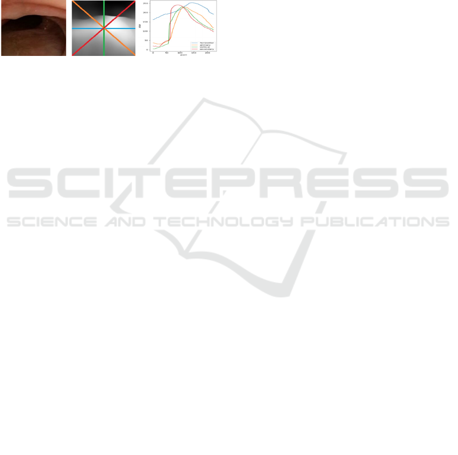
(a) (b) (c)
Figure 1: (a) Original color image, (b) Its depth map with
four lines (Blue: Horizontal Line, Green: Vertical Line,
Orange: Primary Diagonal Line, and Red: Secondary
Diagonal Line), and (c) Grey-scale value plots for the four-
lines.
The main contributions of this work are as
follows. First, we propose to use depth maps for an
image comparison for the first time to the best of our
knowledge. Second, we propose a function to
compare two depth maps very effective for the first
time as far as we know. The rest of the paper is
organized as follows. Section 2 discusses the related
work. Section 3 describes the proposed methodology.
Section 4 shows our experimental results. Finally,
Section 5 summarizes our concluding remarks.
2 RELATED WORK
In this section we provide a brief overview of recent
studies about depth estimation. We use the result of
these studies in our technique.
Almost all existing architectures for depth
estimation are based on convolutional architectures
with an encoder and a decoder. Encoders
progressively downsample the input image to extract
features at multiple scales. However, downsampling
has distinct drawbacks that are particularly salient in
depth estimation tasks. That is feature resolution and
granularity are lost in the deeper stages of the model
and can thus be hard to recover in the decoder (Ranftl
et al., 2021). Instead of using the downsampling, the
authors of (Ranftl et al., 2021) proposed to use vision
transformer (ViT) which foregoes explicit
downsampling operations after an initial image
embedding has been computed and maintains a
representation with constant dimensionality
throughout all processing stages. They reported a
performance increase of more than 28% when
compared to the top-performing fully-convolutional
network on the various datasets.
A conditional generative adversarial network,
Pix2pix based method was proposed to transform
monocular endoscopic image to depth map (Rau et
al., 2019). To overcome the lack of labelled training
data in endoscopy, the authors proposed to use
simulation environments and to additionally train the
generator and discriminator of the model on
unlabelled real video frames in order to adapt to real
colonoscopy environments. They reported promising
results on synthetic, phantom and real datasets and
showed that generative models outperform
discriminative models when generating depth maps
from colonoscopy images, in terms of both accuracy
and robustness.
A method using DenseNet-169 was proposed in
(Alhashim & Wonka, 2018) to generate a high-
resolution depth map given a single RGB color image
with the help of transfer learning. Following the
standard encoder-decoder architecture, the authors
leverage features extracted using high performing
pre-trained networks when initializing their encoder
along with augmentation and training strategies that
lead to more accurate results. They reported that the
proposed method with fewer parameters and training
iterations, outperformed the other two methods
(Laina et al., 2016; Fu et al., 2018) on two datasets.
We used these three approaches discussed above
to generate depth maps for the proposed work. For
convenience, we call the approach in (Ranftl et al.,
2021) as ‘MiDas’, the approach in (Rau et al., 2019)
as ‘Pix2pix’, and the approach in (Alhashim &
Wonka, 2018) as ‘DenseNet-169’.
3 PROPOSED METHOD
We discuss Depth map generation, feature extraction,
and comparison in this section.
3.1 Depth Map Generation
For MiDas we used the code from the web page
(https://github.com/isl-org/dpt) provided in (Ranftl et
al., 2021). We implemented the code with Python 3.7,
PyTorch 1.8.0, OpenCV 4.5.1, and PyTorch Image
Models (timm 0.4.5) per the webpage
(https://github.com/isl-org/dpt). We generated depth
BIOSIGNALS 2023 - 16th International Conference on Bio-inspired Systems and Signal Processing
302

map of our input image by calling the monocular
depth estimation model.
For Pix2pix we used code from TensorFlow
GitHub page which cites the original paper (Isola et
al., 2017) for the implementation (https://
www.tensorflow.org/tutorials/generative/Pix2pix).
For DenseNet-169 we used code from the web page
(https://github.com/ialhashim/DenseDepth) provided
in (Alhashim & Wonka, 2018).
To generate depth maps using Pix2pix and
DenseNet-169, we needed to train them using a
relevant data while MiDas does not need any training.
We used the dataset in (http://cmic.cs.
ucl.ac.uk/ColonoscopyDepth/) provided in (Rau et al.,
2019). This dataset has 16,016 synthetic colonoscopy
images with their corresponding ground truth depth
map images. We split these images to training
samples: 10,346, validation samples: 4,435, and
testing samples: 1,235. We used these three methods
(MiDas, Pix2pix, DenseNet-169) to generate depth
map images for the experiments, and their
performance comparison is reported in Section 4.
3.2 Feature Extraction and Depth Map
Comparison
To compare depth map images, four straight lines are
extracted as discussed before (see Figure 1). Each
point in the four lines has a grey-scale value in its
depth map. Assume that a given image, A is a square
size of S (width) × S (height) pixels in which its width
and height are same. It consists of S
2
pixels in which
a pixel is denoted as p
ij
where i is a row number and j
is a column number. Horizontal Line (HL), Vertical
Line (VL), Primary Diagonal Line (PL), and
Secondary Diagonal Line (SL) of an image A are
defined as follows.
HL
A
= {p
A
ij
} where i = 


, j = 1, 2, … S (1)
VL
A
= {p
A
ij
} where i = 1, 2, … S, j = 


 (2)
PL
A
= {p
A
11
, p
A
22
, p
A
33
, … p
A
SS
} (3)
and
SL
A
= {p
A
1S
, p
A
2(S-1)
, p
A
3(S-2)
, … p
A
S1
} (4)
All the four lines have the same number of pixels,
which are used to derive features to represent a given
image.
A comparison between two given images, Image
A and Image B can be a comparison between the four
lines from Image A and the four corresponding lines
from Image B. A difference (distance) between Image
A and Image B, D
AB
can be calculated using Mean
Absolute Error (MAE) (Willmott et al., 2005) and
defined as follows.
(5)
where,
HL
A
−HL
B
= |p
A
ij
−p
B
ij
| where i=


, j = 1, 2, … S (6)
VL
A
−VL
B
= |p
A
ij
−p
B
ij
| where i = 1, 2, … S, j = 


 (7)
PL
A
−PL
B
= |p
A
11
−p
B
11
|+| p
A
22
−p
B
22
|
+ |p
A
33
−p
B
33
| + … + |p
A
SS
−p
B
SS
|
(8)
SL
A
−SL
B
= |p
A
1S
−p
B
1S
| + | p
A
2(S-1)
−p
B
2(S-1)
|
+ |p
A
3(S-2)
−p
B
3(S-2)
| + … + |p
A
S1
−p
B
S1
|
(9)
Choosing an effective comparison method to
measure the difference (distance) between the two
sets of the four lines is challenging. We tested several
different methods (see Equations (5), (10) – (12)
below) to calculate the difference (distance).
Equation (10) is using Root Mean Square Error
(RMSE - Willmott et al., 2005). Equation (11) called
Metric1 is calculating absolute differences between
the first derivatives of the feature lines (Equations (1),
(2), (3), (4)), and taking a summation of those
differences. Equation (12) called Metric2 is
calculating a difference (distance) in the same way as
Equation (11), using the second derivatives instead.
Among them, MAE in Equation (5) provided a better
accuracy (i.e., F1 score) compared to the others. More
details can be found in Section 4.4.
(10)
(11)
(12)
4 EXPERIMENTS AND RESULTS
In this section we discuss the datasets used for the
experiments, an accuracy comparison of the three
depth map generation methods discussed in Section
3, and a performance evaluation of the proposed
feature extraction with deep learning-based feature
extraction method. We used a workstation with
Intel(R) Core (TM) i7–10700 CPU @ 2.9 GHz 8
Core(s), 16 Logical Processor(s), and NVIDIA
Geforce RTX 2070 Super with 8GB RAM for our
experiments.
𝐷
𝐴
𝐵
𝑀𝐴𝐸
=
1
𝑆
×(
(
𝐻𝐿
𝐴
−𝐻𝐿
𝐵
)
+
(
𝑉𝐿
𝐴
−𝑉𝐿
𝐵
)
+
(
𝑃𝐿
𝐴
−𝑃𝐿
𝐵
)
+
(
𝑆𝐿
𝐴
−𝑆𝐿
𝐵
)
)
𝐷
𝐴
𝐵
𝑅𝑀𝑆𝐸
=

1
𝑆
×((𝐻𝐿
𝐴
−𝐻𝐿
𝐵
)
2
+(𝑉𝐿
𝐴
−𝑉𝐿
𝐵
)
2
+(𝑃𝐿
𝐴
−𝑃𝐿
𝐵
)
2
+(𝑆𝐿
𝐴
−𝑆𝐿
𝐵
)
2
2
𝐷
𝐴
𝐵
𝑀𝑒𝑡𝑟𝑖𝑐1
=

𝑑
𝑑𝑥
(𝐻𝐿
𝐴
)−
𝑑
𝑑𝑥
(𝐻𝐿
𝐵
)

+

𝑑
𝑑𝑥
(𝑉𝐿
𝐴
)−
𝑑
𝑑𝑥
(𝑉𝐿
𝐵
)

+

𝑑
𝑑𝑥
(𝑃𝐿
𝐴
)−
𝑑
𝑑𝑥
(𝑃𝐿
𝐵
)

+

𝑑
𝑑𝑥
(𝑆𝐿
𝐴
)−
𝑑
𝑑𝑥
(𝑆𝐿
𝐵
)

𝐷
𝐴
𝐵
𝑀𝑒𝑡𝑟𝑖𝑐2
=

𝑑
2
𝑑𝑥
2
(𝐻𝐿
𝐴
)−
𝑑
2
𝑑𝑥
2
(𝐻𝐿
𝐵
)

+

𝑑
2
𝑑𝑥
2
(𝑉𝐿
𝐴
)−
𝑑
2
𝑑𝑥
2
(𝑉𝐿
𝐵
)

+

𝑑
2
𝑑𝑥
2
(𝑃𝐿
𝐴
)−
𝑑
2
𝑑𝑥
2
(𝑃𝐿
𝐵
)

+

𝑑
2
𝑑𝑥
2
(𝑆𝐿
𝐴
)−
𝑑
2
𝑑𝑥
2
(𝑆𝐿
𝐵
)

Content Based Image Retrieval Using Depth Maps for Colonoscopy Images
303

4.1 Datasets
We used two datasets for the experiments. The first
dataset (Rau et al., 2019) has 16,016 synthetic
colonoscopy images with their corresponding ground
truth depth map images. More details of the dataset
can be found in the paper (Rau et al., 2019) as
mentioned in Section 3.1. From this dataset, we
selected 200 images in which there are 20 groups with
10 images per group. For convenience, we call it
Dataset1. All images in one group are all similar in
term of their contents (i.e., their surface topology).
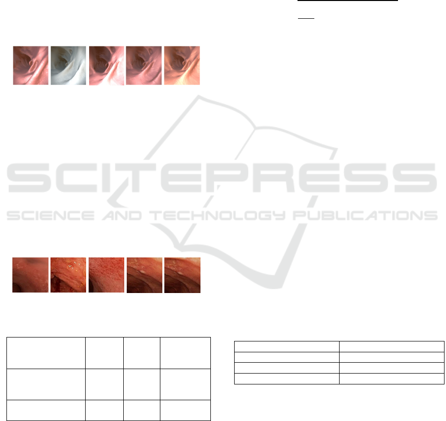
Figure 2 shows five similar images of one group in
this dataset. The resolution of each image is 256
× 256 pixels.
Figure 2: Five similar images in one group from Dataset1.
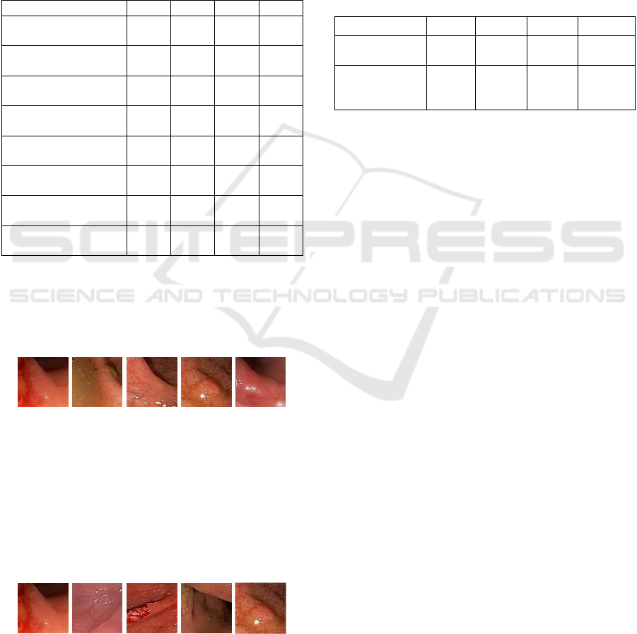
The second dataset has 140 real colonoscopy
images which was used in our previous work
(Author1; Author2; Author3; Author4; Author5;
Author6). For this dataset, we selected 140 images
from 140 colonoscopy procedures to create a more
practical and challenging dataset, in which there are
28 groups with 5 images per group. For convenience,
we call it Dataset2. All images in one group are all
similar in terms of their contents (i.e., their surface
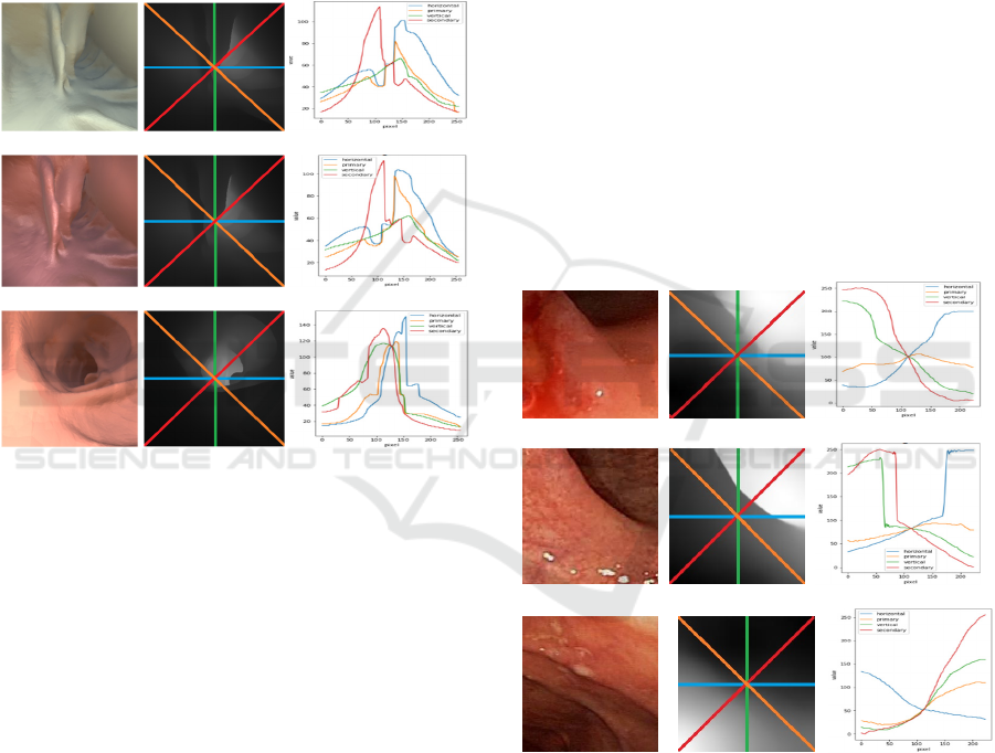
topology). Figure 3 shows five images of one group
in this dataset. The resolution of each image is 224
× 224 pixels. Table 1 summarizes these two datasets.
Figure 3: Five similar images in one group from Dataset2.
Table 1: Dataset details.
Dataset type No. of
Images
No. of
groups
No. of
frames per
groups
Synthetic
colonoscopy
ima
g
e
(
Dataset1
)
200 20 10
Real colonoscopy
image (Dataset2)
140 28 5
4.2 Depth Map Generation
The dataset of the synthetic colonoscopy images
already has their corresponding ground truth depth
map images. However, the dataset with the real
colonoscopy images does not have any depth map, so
we need to generate them. We discussed the three
methods generating depth maps in Section 3.1. Here,
we compared the performance of these methods to
find the best method. First, we applied the three
methods to the synthetic colonoscopy images in
Dataset1 and generated their corresponding depth
map images. And the generated depth maps were
compared with the corresponding ground truth depth
map images using Root Mean Square Error (RMSE)
as follows.
𝑅𝑀𝑆𝐸=

1
𝑀x𝑁
𝐼
(
𝑖,𝑗
)
−𝐾
(
𝑖,𝑗
)


,
,
(13)
where I and K are two images to be compared, the
resolution of each image is M (width) x N (height)
pixels. RMSE is a square root of an average of pixel
differences in the same position. Its value is always
non-negative, and a value closed to zero indicates that
two images are very similar. We calculated a mean
RMSE value for all 200 images in Dataset1. We did
this testing for Dataset1 since Dataset2 does not have
any ground truth depth map images, so there is
nothing to be compared.
Table 2 shows that the mean RMSE values from
the three depth map generation methods are very
close to zero, which indicates all the methods provide
reasonable accuracies. The mean RMSE value of
MiDas is a bit larger than those of the other two
methods. These two methods (Pix2pix and
DenseNet-169) were trained using Dataset1 and
tested with 200 images (not used for training) in
Dataset1. Pix2pix and DenseNet-169 are more
accurate since the training and testing images are
from the same synthetic image dataset, but MiDas
was not trained using any dataset since its structure
does not need any training.
Table 2: Comparison of three depth map generation
methods with their mean RMSE values using Dataset1.
Depth Map method Mean RMSE value
MiDas 0.030345
Pix2pix 0.012239
DenseNet-169 0.016127
4.3 Feature Extraction and
Comparison Examples
In this section, we show some examples about the
feature extraction and comparison discussed in
Section 3.2. The two synthetic images from Dataset1
in Figure 4(a) and (b) are very similar in terms of their
surface topology even if they are different in terms of
BIOSIGNALS 2023 - 16th International Conference on Bio-inspired Systems and Signal Processing
304

their colors. The image in Figure 4(c) is not similar
with them. Figure 4(d), (e) and (f) show their
corresponding ground truth depth maps and four
lines. Figure 4(g), (h) and (i) are showing their
corresponding grey-scale value plots for the four-
lines. The difference (distance) between the two
images in Figure 4(a) and (b) using Equation (5) is
24.39. The same difference (distance) between the
two images in Figure 4(a) and (c) using Equation (5)
is 85.14. This means that Figure 4(a) is relatively
more similar with Figure 4(b), but it is less similar
with Figure 4(c).
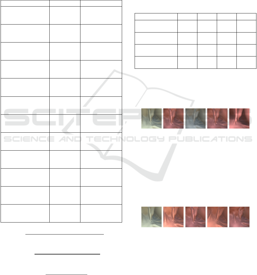
(a) (d) (g)
(b) (e) (h)
(c) (f) (i)
Figure 4: (a), (b) (c): Original Color Images from Dataset1,
(d), (e), (f) Corresponding depth maps with four lines, and
(g), (h), (i): Corresponding Grey-scale value plots for the
four-lines.
The two real Colonoscopy images from Dataset2
in Figure 5(a) and (b) are very similar in term of their
surface topology. The image in Figure 5(c) is not
similar with them. Figure 5(d), (e) and (f) show their
corresponding depth maps and four lines. These depth
maps were generated using MiDas. Figure 5(g), (h)
and (i) show their corresponding grey-scale value
plots for the four-lines. The difference (distance)
between the two images in Figure 5(a) and (b) using
Equation (5) is 78.08. The same difference (distance)
between the two images in Figure 5(a) and (c) using
Equation (5) is 411.60. This means that Figure 5(a) is
relatively more similar with Figure 5(b), but it is less
similar with Figure 5(c).
4 .4 Depth Map Comparison Results
For a comprehensive comparison, we compared our
proposed feature-based method with a deep learning
based CBIR method. In this method, Resnet50 (He et
al., 2016) was used as a feature extractor. This feature
extractor collects a feature vector of 1,024
dimensions for each image. Euclidian distance was
used to calculate a similarity between the feature
vectors of images.
These two methods (Proposed feature-based and
Resnet50 feature-based) were applied to the different
Image sets such as the ground truth depth maps of
Dataset1, the depth maps generated using the three
depth map generation methods in Section 3.1 applied
to Dataset2, and the original color images from
Dataset1 and Dataset2. We included the original color
images from Dataset1 and Dataset2 for a fair and
comprehensive comparison with the Resnet50 based
method. All these cases are summarized in Table 3
below. For convenience, we call the proposed feature
based method as DepthSim (DS), and the Resnet 50
feature based method as Resnet50 (R50).
(a) (d) (g)
(b) (e) (h)
(c) (f) (i)
Figure 5: (a), (b) (c): Original Color Images from Dataset1,
(d), (e), (f) Corresponding depth maps with four lines, and
(g), (h), (i): Corresponding Grey-scale value plots for the
four-lines.
We report the F1 score (Alsmadi et al., 2017) since it
is a combination of Precision and Recall, which are
defined as follows. A high F1 score value is desirable.
For both Dataset1 and Dataset2, we tested four
different query types (Top1, Top2, Top3 and Top4).
Top1 means a single most similar image is retrieved
Content Based Image Retrieval Using Depth Maps for Colonoscopy Images
305

using the corresponding method, and we check if it is
similar with the given query image, in other words, if
it is in the same group of the query image. Similarly,
Top2, Top3 and Top4 mean most similar two, three
and four images are retrieved, and we check if they
are in the same group of the query image.
Table 3: All cases for two methods applied to Dataset1 and
Dataset2.
Cases Methods Images used
Case 1
(DS-Dep-D1)
DepthSim
(DS)
Ground truth
Depth maps in
Dataset1
Case 2
(R50-Dep-D1)
Resnet50
(R50)
Ground truth
Depth maps in
Dataset1
Case 3
(DS-RGB-D1)
DepthSim
(DS)
Original color
Images in
Dataset1
Case 4
(R50-RGB-D1)
Resnet50
(R50)
Original color
Images in
Dataset1
Case 5
(DS-MiDas-D2)
DepthSim
(DS)
Depth maps by
MiDas for
Dataset2
Case 6
(R50-MiDas-D2)
Resnet50
(R50)
Depth maps by
MiDas for
Dataset2
Case 7
(DS-DenseNet-D2)
DepthSim
(DS)
Depth maps by
DenseNet-169
for Dataset2
Case 8
(R50-DenseNet-D2)
Resnet50
(R50)
Depth maps by
DenseNet-169
for Dataset2
Case 9
(DS-Pix2pix-D2)
DepthSim
(DS)
Depth maps by
Pix2pix for
Dataset2
Case 10
(R50-Pix2pix-D2)
Resnet50
(R50)
Depth maps by
Pix2pix for
Dataset2
Case 11
(DS-RGB-D2)
DepthSim
(DS)
Original color
Images in
Dataset2
Case 12
(R50-RGB-D2)
Resnet50
(R50)
Original color
Images in
Dataset2
(14)
(15)
(16)
Table 4 shows F1 scores for Case1 (DS-Dep-D1)
through Case 4 (R50-RGB-D1) in Table 3, and
indicates the proposed feature-based method
performs better than Resnet50 feature-based method
for all different image sets from Dataset1. As seen in
Table 4, the proposed method achieves around 86.8 ~
92.5 % of accuracy on the ground truth depth map
images from Dataset1.
Table 4: Two methods and their accuracies of four different
retrievals on Dataset1.
Experiment Top1 Top2 Top3 Top4
Case 1
(DS-Dep-D1)
0.925 0.905 0.883 0.868
Case 2
(R50-Dep-D1)
0.855 0.793 0.742 0.705
Case 3
(
DS-RGB-D1
)
0.695 0.633 0.567 0.524
Case 4
(R50-RGB-D1)
0.520 0.450 0.401 0.368
Figure 6 shows an example of a query image
(Figure 6(a) from Dataset1) and the retrieved images
(Figure 6(b), (c), (d) and (e)) using the proposed
method. They are all very similar in terms of surface
topology regardless of their colors.
(a) (b) (c) (d) (e)
Figure 6: (a) query image, (b), (c), (d), and (e) retrieved
images based on the proposed method.
Figure 7 shows an example of a query image and
retrieved images. Figure 7(a) is the query image
(same image in Figure 6 (a)), and Figure 7(b), (c), (d)
and (e) are retrieved images using the Resnet50 based
method. Only Figure 7 (c) is similar with the query
(Figure 7 (a)). All others are not very similar in terms
of surface topology.
(a) (b) (c) (d) (e)
Figure 7: (a) query image, (b), (c), (d), and (e) retrieved
images based on Resnet50 based method.
Table 5 shows F1 scores for Case 5 (DS-MiDas-D2)
through Case 12 (R50-RGB-D2), and indicates the
proposed feature-based method outperforms the
Resnet50 feature-based method for all different
image sets from Dataset2. As seen in Table 5, the
proposed method achieves around 86.9 ~ 92.8 % of
𝑅𝑒𝑐𝑎𝑙𝑙=
𝑛𝑢𝑚𝑏𝑒𝑟 𝑜𝑓 𝑠𝑖𝑚𝑖𝑙𝑎𝑟 𝑖𝑚𝑎𝑔𝑒𝑠 𝑟𝑒𝑡𝑟𝑖𝑒𝑣𝑒𝑑
𝑡𝑜𝑡𝑎𝑙 𝑛𝑢𝑚𝑏𝑒𝑟 𝑜𝑓 𝑠𝑖𝑚𝑖𝑙𝑎𝑟 𝑖𝑚𝑎𝑔𝑒𝑠 𝑖𝑛 𝑑𝑎𝑡𝑎𝑏𝑎𝑠𝑒
𝑃𝑟𝑒𝑐𝑖𝑠𝑖𝑜𝑛=
𝑛𝑢𝑚𝑏𝑒𝑟 𝑜𝑓 𝑠𝑖𝑚𝑖𝑙𝑎𝑟 𝑖𝑚𝑎𝑔𝑒𝑠 𝑟𝑒𝑡𝑟𝑖𝑒𝑣𝑒𝑑
𝑡𝑜𝑡𝑎𝑙 𝑛𝑢𝑚𝑏𝑒𝑟 𝑜𝑓𝑖𝑚𝑎𝑔𝑒𝑠 𝑟𝑒𝑡𝑟𝑖𝑒𝑣𝑒𝑑
𝐹1 𝑠𝑐𝑜𝑟𝑒=
2×(𝑝𝑟𝑒𝑐𝑖𝑠𝑖𝑜𝑛×𝑟𝑒𝑐𝑎𝑙𝑙)
𝑝𝑟𝑒𝑐𝑖𝑠𝑖𝑜𝑛+ 𝑟𝑒𝑐𝑎𝑙𝑙
BIOSIGNALS 2023 - 16th International Conference on Bio-inspired Systems and Signal Processing
306

accuracy on the depth maps by MiDas for Dataset2,
which indicates that our proposed method is
promising for practical use. As seen in Cases 5 (DS-
MiDas-D2), 7 (DS-DenseNet-D2), and 9 (DS-
Pix2pix-D2) in Table 5, the depth maps generated by
MiDas provided much better accuracies. The reason
is that Pix2pix and DenseNet-169 trained using
Dataset1 were applied to Dataset2, so they did not
generate accurate depth maps.
Table 5: Two methods and their accuracies of four different
retrievals on Dataset2.
Experiment Top1 Top2 Top3 Top4
Case 5
(
DS-MiDas-D2
)
0.928 0.925 0.907 0.869
Case 6
(
R50-MiDas-D2
0.386 0.318 0.269 0.243
Case 7 (DS-
DenseNet-D2)
0.135 0.139 0.114 0.107
Case 8
(
R50-DenseNet-D2
)
0.107 0.096 0.090 0.086
Case 9
(
DS-Pix2
p
ix-D2
)
0.121 0.143 0.131 0.127
Case 10
(R50-Pix2pix-D2)
0.093 0.103 0.095 0.082
Case 11
(DS-RGB-D2)
0.143 0.114 0.114 0.100
Case 12
(
R50-RGB-D2
)
0.114 0.104 0.093 0.086
Figure 8 shows an example of query and retrieval in
which Figure 8(a) is a query image in Dataset2, and
Figure 8(b), (c), (d) and (e) are retrieved images using
the proposed method. They are all very similar in
terms of surface topology regardless of their colors.
(a) (b) (c) (d) (e)
Figure 8: (a) query image, (b), (c), (d), and (e) retrieved
images based on the proposed method.
Figure 9 shows an example of query and retrieval in
which Figure 9(a) is a query image (same image in
Figure 8 (a)), and Figure 9(b), (c), (d) and (e) are
retrieved images using Resnet50 based method. All
retrieved images are not very similar in terms of
surface topology.
(a) (b) (c) (d) (e)
Figure 9: (a) query image, (b), (c), (d), and (e) retrieved
images based on the Resnet50 based method.
We compared four distance functions (Equation
(5), Equations (10), (11) and (12)) discussed in
Section 3.2, and their results are in Table 6. Table 6
shows Cases 1 (DS-Dep-D1) and 5 (DS-MiDas-D2)
in which the proposed method was applied to the
ground truth depth maps in Dataset1, and the depth
maps by MiDas for Dataset2. The F1-scores in Table
6 are the results of Top1 query where a most similar
single image is retrieved. As seen in table 6, Equation
(5) provided a best result among them.
Table 6: Comparison of four distance functions and their
F1-scores.
Experiment Eq. (5)
Eq. (10) Eq. (11) Eq. (12)
Case1
(
DS-De
p
-D1
)
0.925 0.925 0.380 0.130
Case5
(DS-MiDas-
D2
)
0.928 0.907 0.579 0.421
5 CONCLUDING REMARK AND
FUTURE WORK
This paper presents a new technique to compare
images in which low-level visual features (i.e., color,
shape, texture, and spatial layout) or Convolutional
Neural Network features are not effective. This new
technique finds image similarity in terms of the
surface topology using the depth map images. The
experiments based on synthetic and real colonoscopy
images show that the proposed technique achieves
around 90% accuracy, indicating it can potentially be
used in practice. In the future, to improve the
accuracy of the proposed method, we will consider an
enhancement of the depth map generation methods
discussed in Section 3.1, and investigate a different
method (i.e., Jensen–Shannon divergence (Frank
Nielsen, 2021)) of measuring the similarity between
two lines as discussed in Section 3.2.
ACKNOWLEDGEMENTS
For MiDas, we used the code from the web page
(https://github.com/isl-org/dpt), under MIT license.
For Pix2pix, we used the code from TensorFlow
GitHubpage (https://www.tensorflow.org/tutorials/
generative/Pix2pix) under Apache license version
V2.0. For DenseNet-169, we used code from the
webpage (https://github.com/ialhashim/DenseDepth)
under GNU General Public License v3.0. All those
three types of licenses are in the permissive category
Content Based Image Retrieval Using Depth Maps for Colonoscopy Images
307

and free to use for individual. For the synthetic data
(Dataset1 in Table1) we acknowledge (Rau et al.,
2019) for the synthetic dataset based on the condition
to cite their study paper.
REFERENCES
Meenalochini, M., Saranya, K., Rajkumar, G. V., & Mahto,
A. (2018, October). Perceptual hashing for content
based image retrieval. In 2018 3rd International
Conference on Communication and Electronics
Systems (ICCES) (pp. 235-238). IEEE.
Öztürk, Ş. (2021). Class-driven content-based medical
image retrieval using hash codes of deep
features. Biomedical Signal Processing and
Control, 68, 102601.
Chen, W., Liu, Y., Wang, W., Bakker, E., Georgiou, T.,
Fieguth, P., Liu, L., & Lew, M. S. (2021). Deep
Learning for Instance Retrieval: A Survey.
https://doi.org/10.48550/arxiv.2101.11282
Latif, A., Rasheed, A., Sajid, U., Ahmed, J., Ali, N., Ratyal,
N. I., ... & Khalil, T. (2019). Content-based image
retrieval and feature extraction: a comprehensive
review. Mathematical Problems in Engineering, 2019.
Mokter, M.F., Idris , Azeez Idris., Oh, J., Tavanapong, W.,
Wong, J., & Groen, P. C. D. (2022, October). Severity
Classification of Ulcerative Colitis in Colonosco-py
Videos by Learning from Confusion. In 17th
International Symposium on Visual Computing.
Springer, Cham.
Rahman, M. M., Oh, J., Tavanapong, W., Wong, J., &
Groen, P. C. D. (2021, October). Automated Bite-block
Detection to Distinguish Colonoscopy from Upper
Endoscopy Using Deep Learning. In International
Symposium on Visual Computing (pp. 216-228).
Springer, Cham.
Mokter, M. F., Oh, J., Tavanapong, W., Wong, J., & Groen,
P. C. D. (2020, October). Classification of ulcerative
colitis severity in colonoscopy videos using vascular
pattern detection. In International Workshop on
Machine Learning in Medical Imaging (pp. 552-562).
Springer, Cham.
Tejaswini, S. V. L. L., Mittal, B., Oh, J., Tavanapong, W.,
Wong, J., & Groen, P. C. D. (2019, October). Enhanced
approach for classification of ulcerative colitis severity
in colonoscopy videos using CNN. In International
Symposium on Visual Computing (pp. 25-37). Springer,
Cham.
Willmott, C. J., & Matsuura, K. (2005). Advantages of the
mean absolute error (MAE) over the root mean square
error (RMSE) in assessing average model
performance. Climate research, 30(1), 79-82.
Ranftl, R., Bochkovskiy, A., & Koltun, V. (2021). Vision
transformers for dense prediction. In Proceedings of the
IEEE/CVF International Conference on Computer
Vision (pp. 12179-12188).
Ranftl, R., Lasinger, K., Hafner, D., Schindler, K., &
Koltun, V. (2020). Towards robust monocular depth
estimation: Mixing datasets for zero-shot cross-dataset
transfer. IEEE transactions on pattern analysis and
machine intelligence.
Rau, A., Edwards, P. J., Ahmad, O. F., Riordan, P., Janatka,
M., Lovat, L. B., & Stoyanov, D. (2019). Implicit
domain adaptation with conditional generative
adversarial networks for depth prediction in
endoscopy. International journal of computer assisted
radiology and surgery, 14(7), 1167-1176.
Li, Z., & Snavely, N. (2018). Megadepth: Learning single-
view depth prediction from internet photos.
In Proceedings of the IEEE conference on computer
vision and pattern recognition (pp. 2041-2050).
Isola, P., Zhu, J. Y., Zhou, T., & Efros, A. A. (2017). Image-
to-image translation with conditional adversarial
networks. In Proceedings of the IEEE conference on
computer vision and pattern recognition (pp. 1125-
1134).
Alhashim, I., & Wonka, P. (2018). High quality monocular
depth estimation via transfer learning. arXiv preprint
arXiv:1812.11941.
Laina, I., Rupprecht, C., Belagiannis, V., Tombari, F., &
Navab, N. (2016, October). Deeper depth prediction
with fully convolutional residual networks. In 2016
Fourth international conference on 3D vision
(3DV) (pp. 239-248). IEEE.
Fu, H., Gong, M., Wang, C., Batmanghelich, K., & Tao, D.
(2018). Deep ordinal regression network for monocular
depth estimation. In Proceedings of the IEEE
conference on computer vision and pattern
recognition (pp. 2002-2011).
He, K., Zhang, X., Ren, S., & Sun, J. (2016). Deep residual
learning for image recognition. In Proceedings of the
IEEE conference on computer vision and pattern
recognition (pp. 770-778).
Alsmadi, M. K. (2017). An efficient similarity measure for
content based image retrieval using memetic
algorithm. Egyptian journal of basic and applied
sciences, 4(2), 112-122.
Frank Nielsen (2021). "On a variational definition for the
Jensen-Shannon symmetrization of distances based on
the information radius". Entropy. MDPI. 23 (4): 464.
doi:10.3390/e21050485. PMID 33267199.
BIOSIGNALS 2023 - 16th International Conference on Bio-inspired Systems and Signal Processing
308