Estimating Workforce Attrition Rate Parameters: A Controlled

Comparison

Robert Mark Bryce and Jillian Anne Henderson

Defence Research and Development Canada (DRDC)-Centre for Operational Research and Analysis (CORA),

Department of National Defence (DND), 60 Moodie Drive, Ottawa, Canada

Keywords:

Attrition, Workforce Analytics, Memoryless, Survival Time, Stochastic Process, Estimator.

Abstract:

Here we consider workforce attrition rate parameter estimators (three continuous, three discrete), demonstrat-

ing that they originate in the Ordinary Differential Equation (ODE) describing a memoryless survival time

population. This demonstration reveals how to craft estimators and reason about them. Setting up controlled

numerical experiments we test this family of estimators to determine their relative performance, both in steady

state and under dynamic change of population level. Additionally, we ﬁnd the analytic expressions for the

residual error of the estimators which provides insight into their bias properties. Our results suggest that, out

of common simple estimators, the two-point average population and half-intake estimators are robust choices.

1 INTRODUCTION

Determining the attrition properties of a workforce

is informative as a diagnostic (e.g., are more mem-

bers leaving than typical?) and for planning purposes

(e.g., if we want to grow by 10% within three years

how many hires per annum will we need to take on?).

Comparison to peers can be valuable, providing in-

sight on the relative position ones institution holds,

and forecasting is useful for a “heads up” view on in-

stitutional health. To this end having a good estimate

of the attrition rate parameter describing one’s work-

force is valuable, where good means, among other

things, providing precision and accuracy for mod-

elling and forecasting purposes. In this work we com-

pare estimators of the attrition rate parameter which

are in use by various militaries, who have a keen inter-

est in managing occupation levels (sub-populations)

that deliver mandated capability, with the aim of pro-

viding a controlled comparison. To this end we set up

numerical experiments with known attrition rate prop-

erties and quantitatively check the performance of the

estimators.

We take a simple model of workforce attrition

as foundational: workforce attrition is viewed as

a stochastic process. A quasi-stationary survival

time distribution is taken to describe member life-

time within the institution. This viewpoint allows for

stochastic simulations, such as Discrete Event Sim-

ulation (DES), to generate population trajectories via

random assignment of lifetime from the survival dis-

tribution. Notable, the historical record is a particu-

lar realization of a stochastic process describing the

population. The stochastic process view takes the

additional step of positing that other realizations are

informative and meaningful, including future popu-

lation trajectories. The validity of this assumption

hinges on the survival distribution capturing the vari-

ation expected, and, for forecasts, that the institute

and embedding social conditions do not qualitatively

change or show “signiﬁcant” quantitative change over

the forecast horizon.

One key advantage of the stochastic process view

is contact can be made with theory, for the case of a

memoryless population (see Section 2, where the the-

ory is outlined) which maps directly, and uniquely,

to an exponential survival distribution (Feller, 1957).

Furthermore the theoretical framework speaks to the

majority of attrition rate parameter estimators (Sec-

tion 3), with the possible exception of heuristic es-

timators where contact with theory is more opaque.

As the estimators can be viewed as a family which

assumes an identical underlying model (memoryless

attrition) it is expected that all estimators will, broadly

speaking, be in agreement. Despite this one can ex-

pect differences in performance and, for example, one

can imagine some estimators showing bias in various

contexts. To identify possible bias and speak to rel-

ative performance we consider three scenarios: (1)

steady, (2) growing, and (3) reduction of populations,

Bryce, R. and Henderson, J.

Estimating Workforce Attrition Rate Parameters: A Controlled Comparison.

DOI: 10.5220/0011748600003396

In Proceedings of the 12th International Conference on Operations Research and Enterprise Systems (ICORES 2023), pages 82-93

ISBN: 978-989-758-627-9; ISSN: 2184-4372

 2023 by SCITEPRESS – Science and Technology Publications, Lda. Under CC license (CC BY-NC-ND 4.0)

by constructing numerical experiments with known

attrition properties (Section 4). These experiments

mainly consider the “best case”—a memoryless pop-

ulation—as interpretation is facilitated here, but we

also consider a population with a distinctly non-

exponential survival distribution (Canadian Armed

Forces (CAF) Regular Force (Reg F), Primary Re-

serves (P Res), and Naval Warfare Ofﬁcer (NWO)) to

extend analysis and speak to practical issues.

2 MODELS OF ATTRITION

It appears that, in practice, the concept of workforce

attrition is associated with the number of members of

a population leaving in some set period and is mea-

sured by a churn, or attrition, rate. The churn rate is

deﬁned as the number of members who leave on an

interval, out, divided by the population size, P, a con-

ceptually viable deﬁnition. As, in general, the popula-

tion level changes when members leave and, typically,

new members enter over time there are questions re-

garding what “the” population is and there are differ-

ing speciﬁc choices one can make—take the popula-

tion level at the start of the interval, at the end, the

average, etc.

Despite the ambiguity and apparent ad hoc choice

in how to measure attrition, we will show that there is

essentially a single model of attrition—the memory-

less model—plus the stochastic process view, which

can either match this model (when the survival dis-

tribution is exponential) or be general (e.g., non-

parametric distributions such as a histogram or cu-

mulative distribution function (CDF), or parametric

forms). Viewed from the lens of the memoryless

model common means of measuring “attrition rate”,

which we term the attrition rate parameter (for rea-

sons that will become apparent), will be seen as mem-

bers of the same family and which all naturally follow

from the same originating equation.

It should be noted that even a loose deﬁnition of

churn will approximately measure the attrition and,

unless dramatic change in population levels occurs

over the interval in question, these will all be simi-

lar due to the same originating concept. While this is

unarguably true it should be noted that 1) churn rate of

customer contracts or employees, say, is used to make

ﬁnancial and hiring decisions and so bias and error

in estimates can have real impact on decisions, 2) a

careful development will provide a means to select a

“good” means of estimating, as even if the choices are

similar perhaps some are better in some sense, and

3) the development here can speak towards improve-

ments beyond the current estimators in use.

2.1 The Memoryless Model

A simple continuous differential model describing the

change of a homogenous population over time due to

attrition at a rate αP (outﬂow) and a constant intake

rate in (inﬂow) is

= −αP + in (1)

where P

is the time derivative of the population. This

Ordinary Differential Equation (ODE) has an exact

solution

P(t) =



−



−αt

, (2)

where P

is the initial population, as can be veriﬁed by

plugging this solution back into the originating differ-

ential equation. Evaluating the solution (2) at discrete

multiples of the unit time t = 0,1,2. . . we recast (2)

as a recurrence relation and ﬁnd

t+1



−



−α

= P

−α

(1 −e

−α

)

= (1 −γ)P

+ in





(3)

where the last expression foreshadows the corrected

discrete approximation we will consider in the next

section, and which makes use of the mapping between

the continuous time attrition rate parameter and the

discrete time probability γ = 1 −e

−αT

, where T is the

unit time.

Here it is clear that the attrition rate αP is the at-

trition rate parameter α times the population level,

which matches simple dimensional analysis where α

has units of inverse (unit) time and P units of mem-

bers as so multiplied together they have units of a rate

(members per (unit) time leaving).

It should be noted that in (1) a constant intake rate

is assumed. This facilitates solution (2), but does not

lead to meaningful loss of generality as functions with

a ﬁnite number of jump discontinuities can be approx-

imated by piecewise constant functions with arbitrary

precision—one simply solves (1) on each piecewise

constant region.

2.2 Discrete Approximation

Discrete Time Markov Models (DTMMs) have long

been a popular approach to workforce analysis (Seal,

1945; Young and Almond, 1961; Merck and Hall,

1971; Vajda, 1978; Bartholomew and Forbes, 1979),

most likely due to the ease of implementation and

widespread knowledge of Markov chains. However,

they are typically misspeciﬁed in that entry events can

happen between the time steps and therefore as time

Estimating Workforce Attrition Rate Parameters: A Controlled Comparison

steps increase in size error will increasingly accrue.

We will ﬁrst outline the standard discrete time ap-

proach, in the single component workforce case, pro-

vide an approximate correction given in (Okazawa,

2007), and demonstrate the exact correction which re-

covers equation (3).

The basic idea behind the DTMM for workforces

is that entry processes occur at discrete points in time.

For a homogeneous population only two processes

occur: entry into the population, and exit from the

population (for heterogeneous populations ﬂow be-

tween subcomponents also occurs). Entry is treated

deterministically with a set number of entrants en-

tering at the end of a time period, while exit is con-

sidered probabilistically with a given probability of

γ = 1 −e

−αT

of leaving (Vajda, 1978; Bartholomew

and Forbes, 1979); note the explicit relationship with

the continuous time attrition rate parameter. The re-

sult is the following equation describing the popula-

tion over time

t+1

= P

−out + in = (1 −γ)P

+ in, (4)

where out = γP

is the number of personnel who leave,

in expectation, over a time step and in is the intake

occurring at the end of the time period.

Notice that (3) differs from (4) in that in has a

modifying factor—this is due to the discrete time

steps neglecting intake events happening between the

time steps. The main limitation of (4), for modelling

continuous entry into a population, is that entry can

occur between the time steps leading to error. In

(Okazawa, 2007) an approximate correction that ac-

counts for continuous entry between time steps is de-

veloped leading to

t+1

= (1 −γ)P

+ (1 −γ/2)in. (5)

This correction is denoted the “half-intake” formu-

lation for obvious reasons. With regards to this ap-

proximate correction we note that by assuming con-

tinuous intake over the time period one models situa-

tions where entry happens uniformly over time, where

in is considered as an intake density (number who

enter, divided by the time period; for simplicity we

will work with unit time). The density entering at

time t will experience exponential decay for a time of

(1 −t), i.e., to the end of the time step. This modiﬁes

(4) in the following manner

t+1

= (1 −γ)P

in ·e

−α(1−t)

= (1 −γ)P

+ in



1 −e

−α



= (1 −γ)P

+ in





(6)

and (3) is recovered exactly.

Finally, we note that the multiple component

DTMM model is a simple (matrix) extension of the

single component model outlined here (Bartholomew

and Forbes, 1979). While not widely recognized, one

can also directly solve the matrix version of (1) either

exactly (Higham, 2008; Henderson and Bryce, 2019)

or approximately by ﬁnding the Linear Dynamical

System (LDS) associated with the matrix version of

(1) (i.e., use Euler’s method). The LDS is identi-

cal in form with the DTMM, with the discrete tran-

sition probabilities replaced with continuous attrition

rate parameters. Note that as the time step diminishes

to zero the LDS and DTMM converge to the same

(exact) limit. If a continuous entry process describes

a population the continuous model is a better ﬁt than

a discrete time model, and as the LDS is identical in

form to the DTMM the advantages of DTMM (mainly

simple implementation) can be had in the continu-

ous domain while reducing modelling error due to

taking ﬁnite time steps. It should also be noted that

simply reducing the time step towards zero will lead

to improved results, for either approximate approach

(DTMM, LDS).

2.3 The General Formula (GF)

The GF for the attrition rate parameter is an heuris-

tically derived approach (Vincent et al., 2021; Vin-

cent, 2019; Vincent et al., 2018). The GF approach

offers an alternative perspective on attrition to that

taken here; Ref. (Vincent et al., 2021) is a readable

and careful overview of the GF approach which in-

cludes empirical results and reviews prior work.

Brieﬂy, the approach taken is to consider sub-

intervals deﬁned by intake events and imposing the

constraint that the attrition formula should have some

desired properties (namely, the attrition rate parame-

ter is the proportion that departs and the overall rate

is related to the sub-period rates) which leads to

1 −γ =

∏

i=1

+ out

(GF)

where γ is the discrete attrition rate parameter, i in-

dexes the n sub-intervals, p

is the population at the

end of the i-th sub-interval, and out

is the attrition on

the i-th sub-interval.

Note that there is no explicit time scale in the GF

and that a change in sub-interval size does not affect

the measured attrition rate parameter; as the attrition

rate parameter describes the expected time to attrition

there must be a time scale, and so the GF relies on an

implicit unit time (e.g., the measurement period). Fur-

ther note that as intake events deﬁne the sub-intervals

ICORES 2023 - 12th International Conference on Operations Research and Enterprise Systems

these are free fall (no intake) regions, on which dis-

crete time approaches are expected to perform well,

with the important distinction that the time intervals

are not ﬁxed.

2.4 Stochastic Processes

We ﬁrst remark on the relationship γ = 1 −e

−αT

that

maps the continuous attrition rate α to the discrete

one γ. This relationship describes decay between im-

pulse intakes at discrete times and can be obtained

directly from Equation 2 by setting in to zero to ﬁnd

the exponential decay on free fall periods P

−αT

and

noting that the fraction of the initial population re-

maining will be P

(1 −γ) where we introduce γ as

the fraction of the population that will attrite on the

interval. We can generalize our view by considering

the stochastic process perspective where for some ini-

tial population members have lifetimes that will dic-

tate their eventual exit time. Here, for an exponential

survival curve the decay is, by deﬁnition, exponential

and the continuous-discrete relationship holds. A sur-

vival curve is deﬁned as 1 −CDF(t), where CDF(t)

is the cumulative distribution function, and for an ex-

ponential survival curve the distribution is the expo-

nential distribution. We see then that a stochastic

process with an exponential survival distribution will

match, in expectation, the ODE describing a memory-

less population—at least when intake occurs at ﬁxed

discrete times.

We strengthen the connection between a (expo-

nential survival distribution) stochastic processes and

the memoryless population ODE view by noting the

following. First, we do not need intake to occur at

ﬁxed points in time. Rather we can allow variable free

fall periods with boundaries deﬁned by intake events

(e.g., as for the GF), and again the survival curve will

match the ODE, in expectation, on the intervals and

the continuous-discrete relationship holds. Second,

if we have uniform intake of in over a unit time in-

terval than the solution to the ODE with intake rate

in (Equation (2)) is recovered, in expectation, as can

be seen by considering Equation (6) and associated

discussion. We see that a stochastic process, deﬁned

by an exponential survival distribution and (piecewise

constant) uniform intake regions, will have average

behaviour described by the memoryless ODE describ-

ing the population.

One can consider a more general stochastic pro-

cess, where instead of drawing from an exponential

survival distribution we draw from a general distri-

bution and again have uniform piecewise constant in-

take. While the ODE (1) describing a memoryless

population will no longer fully describe the dynam-

ics we can simulate under historical and planned in-

take plans using, for example, DES (Devroye, 1998).

For this work we will be using stochastic simulations

where we uniformly create entry events at a given

annual intake rate, and for each entry draw a sur-

vival time from a distribution (either exponential or

an empirical histogram) to ﬁnd the corresponding exit

event. From a given realization we will measure the

population at an annual frequency, and measure the

outﬂow out on the annual time intervals and use these

measurements to assess attrition rate parameter esti-

mators (see next section). Details on the numerical

experiments are provided in Section 4.

This direct match between a stochastic process

view of the population and the ODE (1) describing

the mean population trajectory, for the appropriate in

proﬁle, is advantageous as one can verify stochastic

simulations against theory in this special (memory-

less population) case (Henderson and Bryce, 2019)

and then extend to more complex survival distribu-

tions (Bryce and Henderson, 2020) if warranted by

modelling needs. In particular, modelling error due

to assuming the memoryless case can be probed; de-

pending on the modelling context this error can be

quite limited (Bryce and Henderson, 2020), and for

mild changes in intake the memoryless assumption is

a reasonable simpliﬁcation.

3 MEASURING α FROM DATA

3.1 Estimators

Provided a model one would like to determine the pa-

rameters, given data. To do this an estimator has to be

constructed. In Equation 1 the instantaneous attrition

rate (outﬂow volume per unit time) is out

= αP(t),

where the prime is used here to emphasize this is a

rate, and we have

out =

out

dt = α

P(t)dt (7)

where we take α as constant and pull it out of the inte-

gral. We can deﬁne an interval (t

−t

), measure the

number out who attrite over this interval, and solve

the integral of the population to obtain an estimator

of the attrition rate parameter

α =

out

P(t)dt

(8)

where we use a hat to emphasize this is an estimator.

Here we focus on simple numerical estimates of

the population integral, as these relate to commonly

Estimating Workforce Attrition Rate Parameters: A Controlled Comparison

used estimators, but we note that the population in-

tegral over an interval can be determined from Hu-

man Resources records and also found for simulated

and forecast populations. We construct three estima-

tors using simple numerical integration schemes on

a single interval, and then introduce three other esti-

mators used in practice. In the following we use an

annual interval, as this is a natural unit for organiza-

tions and human resources, and so (t

−t

) falls out

as it is unit—but is implicitly present.

• Steady State Estimator (Continuous).

We consider the ideal case of a constant (steady

state) population, where P(t) = P

P(t)dt =

exactly. This gives

out

. (E0)

This estimator is only suitable when the popula-

tion does not change which, in general, we do not

expect to hold even in steady state (due to stochas-

tic ﬂuctuations). The change in population levels

is what motivates a need for various estimators.

Here we do not empirically test E0, due to it’s

limited applicability, but instead derive it to make

contact with intuitive development of estimators,

which often start with E0 based on the conceptual

deﬁnition of attrition, as well as to support its use

in reasoning about steady state conditions.

• Left Estimator (Continuous).

We consider the left Riemann sum on a single in-

terval,

P(t)dt ≈ P(t

) which, substituting into

Equation 8, leads to

out

(E1)

where we use P

to denote P(t

) for convenience.

The Korea Institute for Defence Analyses uses

this estimator (Vincent, 2019).

• Mean Estimator (Continuous).

Using the trapezoidal rule on a single interval

P(t)dt ≈ (P(t

) + P(t

))/2 leads to

out

mean

2 out

+ P

(E2)

where we again change notation for the starting

and end populations on the interval. We denote

this the mean estimator as the two-point average

over the interval is used to estimate the popula-

tion. This estimator is used by the Australian

Army, Swedish Defence Research Agency, and

U.K.’s Royal Air Force (Vincent, 2019).

• Right Estimator (Continuous).

Using the right Riemann sum on a single interval

leads to

out

(E3)

where we use P

for P(t

• Half-Intake Estimator (Discrete).

out

+ in/2

(E4)

This estimator is used by the CAF (Vincent,

2019), and is a correction of a DTMM approxi-

mation (Okazawa, 2007). This is a semi-discrete

model as it does not correspond to a probability, as

in the discrete case, as can be seen by considering

the high attrition steady state limit where in and

out P

such that the estimate could take on val-

ues > 1. At lower attrition and time steps the esti-

mator should become increasingly well behaved.

• Markov Estimator (Discrete).

Here attrition is measured in free fall conditions

(no intake) over a single time step.

P(t)dt =

γ, which is obtained by plugging in the solution

to Equation 1 (i.e., Equation 2) with an intake rate

of zero, and using the discrete-continuous map

deﬁnition of γ. Plugging this into Equation 8 al-

lows us to cancel the α from both sides and move

the γ to the left-hand side and we ﬁnd

out

. (E5)

Note that free fall conditions is misspeciﬁed when

there is a non-zero intake rate, e.g. a discrete time

step process is misspeciﬁed for continuous entry

populations. This estimator is recommended in

(Bartholomew and Forbes, 1979) as this form is

known to be the Maximum Likelihood Estima-

tion (MLE) for DTMM (Anderson and Goodman,

1957).

• General Formula (GF) Estimator (Discrete).

Here we start as for the Markov estimator. In free

fall the following holds: P

= P

−out, we use

this constraint to ﬁnd the GF estimator as follows.

Apply the constraint to the numerator and denom-

inator of E5, and simplify to get the single time

interval GF estimator

= 1 −

+ out

. (E6)

As for the Markov estimator this will be misspec-

iﬁed for non-zero intake over an interval. This es-

timator is recommended in Ref. (Vincent et al.,

2021).

ICORES 2023 - 12th International Conference on Operations Research and Enterprise Systems

It should be noted that, in general, there can be confu-

sion between whether the discrete or continuous attri-

tion rate parameter is being estimated from the data,

for example (E1) and (E5) are identical in form but

measure the continuous and discrete rate parameters,

respectively. For comparison and modelling purposes

it is important to be clear on this point. For clarity

here we map all discrete estimates back to the contin-

uous domain by inverting γ = 1 −e

−αT

, this allows

all estimators to be directly compared to each other

and to the set attrition rate. For example, for (E5) we

report as

= −ln(1 −

) = −ln(1 −

out

The discrete approach follows the same underly-

ing attrition model and is a discrete time approxima-

tion to the ODE describing a memoryless population,

and so the discrete estimators (E4–E6) fall into the

same fundamental family of estimators. For ﬁnite

time steps these estimators will have discretization er-

ror, but for small α this error will be small and in gen-

eral all estimators are expected to converge and per-

form well in the vanishing α limit.

We can relate the three continuous estimators we

constructed from single step numerical integration, as

out

2(P

+ P

)

2out

(9)

and so

. (10)

We note the following mnemonic to help iden-

tify which index refers to which estimator: the left

estimator takes the ﬁrst point in the interval (“one”),

the mean estimator uses the midpoint approximation

(“two”), and the right estimator takes the last point

(“three”).

3.2 Residual Error of Estimators

As we are considering the performance of the estima-

tors we derive analytic forms for the expected residual

error. We ﬁrst consider correlation effects in combi-

nation with steady state considerations to ﬁnd residu-

als for the continuous estimators, and then use steady

state arguments to ﬁnd residuals for the discrete esti-

mators. We note that the residual is equivalent to the

bias of the estimator, and emphasize that the residuals

apply in steady state.

3.2.1 Residual Error for Continuous Estimators

Observe the following. In steady state if there is an

atypically large loss in an interval (out) then the pop-

ulation level at the end (P

) will be smaller than nor-

mal; in this case E3 be strongly effected as the nu-

merator increases while the denominator decreases.

Likewise for unusually small outﬂow. This makes E3

strongly (anti) correlated with P

. Note that both E1

and E2 do not suffer from such a strong effect, and in

particular we expect less correlation for E1 and mod-

erate correlation for E3. We will make use of these

observations below.

To assess the performance of the estimators we

will consider the residual error between the average

over simulations (expectation) and the set α. We de-

rive an analytic expression for the residual, making

use of covariance between estimators and population

level, where we use

∗

and P

∗

as placeholders

COV [

∗

] ≡ E[

∗

] −E[

∗

]E[P

∗

] (11)

where E is the expectation. We expand the deﬁnition

∗

and use the steady state result E[P

∗

] = in/α (see

E0)

COV [

∗

] = E[

out

∗

] −E[

∗

]

(12)

in steady state E[out] = in and so

COV [

∗

] = in −E[

∗

]

(13)

multiplying both sides by −α/in we obtain the fol-

lowing for the residual

∗

] −α = −

COV [

∗

]. (R1–R3)

Note that the observations above suggests that the

residual (error) of E3 will be the largest, E1 the small-

est, and E2 intermediate. As we expect anti correla-

tion the form of the residual indicates a positive bias.

It is worth noting that α can be considered as a

time dilation factor (see Equation 2) and so as α ap-

proaches zero we expect ‘time to slow’ relative to

larger α. The result is P

∗

will be quasi-static in a

time region and out (and hence

∗

) will be ≈ 0, and

so the covariance in Equation R1–R3 will go to zero

likewise. Applying the time dilation argument in the

other direction, we expect covariance to grow with α.

3.2.2 Residual Error for Discrete Estimators

To ﬁnd the residual of the discrete estimators we con-

sider steady state arguments, where we use E0 to as-

sert that E[P

∗

] = in/α and the fact that E[out] = in

to eliminate all occurrences of variables, other than

α, in the estimator equations (where we take the ex-

pectation to allow elimination). Applying algebraic

simpliﬁcation leads to the following:

• Half intake estimator residual

] −α = −ln



1 −

1 +



−α. (R4)

Estimating Workforce Attrition Rate Parameters: A Controlled Comparison

• Markov estimator residual

] −α = −ln(1 −α) −α. (R5)

• General Formula (GF) estimator residual

] −α = ln (1 + α) −α. (R6)

By inspection, we see that the Markov and half-intake

estimator residuals will have a positive bias (i.e., the

estimates are expected to be too large), which disap-

pears as α goes to zero. In contrast the GF estimator

residual is negative in expectation, and again goes to

zero as α does.

We note two simplifying aspects about our deriva-

tion of discrete residual error here. First, we do not

consider correlation effects as we expect (and will see

in Section 4) these will be small relative to the mis-

speciﬁcation error inherent in the discrete estimators.

Second, we take E[1/X] ≈ 1/E[X] which is strictly

untrue (Jensen’s inequality) as we, again, expect the

introduced error to be relatively small.

4 NUMERICAL EXPERIMENTS

To test the performance of the estimators we will mea-

sure them on a workforce population for which we

control the parameters. We chose a single component

(i.e., homogenous) population described by the ODE

(1) for simplicity allowing us to investigate bias due

to estimator choice without complicating factors.

As previewed in Section 2.4, we use stochastic

simulations to create realizations of our population

which is deﬁned by a characteristic survival distribu-

tion and grown from zero to steady state under a con-

stant intake rate. After considering this steady state

regime we introduce an intake rate step growth or de-

cline to examine the dynamic regime. The estimators

from Section 3.1 were measured over each simula-

tion run (1000 replications) and on an annual interval

(chosen as it is a common frequency used in insti-

tutional planning and reporting). Estimator bias was

then determined by examining the residual error be-

tween the ﬁnal mean estimator,

α, and the set attrition

rate parameter, α.

We start with the case of memoryless (exponen-

tial) attrition, where the attrition rate parameter is

varied over a wide range in order to observe both

typical and more extreme, but plausible, behaviour

(α ∈ [0.01,2.0]). We then extend the experiment with

the general stochastic process case by using historical

personnel records of several CAF sub-groups.

The CAF considers various sub-populations of in-

terest for strategic planning and here we include the

two largest groups: Regular Force (Reg F) and Pri-

mary Reserves (P Res) (∼120,000 and ∼80,000 ob-

servations, respectively). Also included is the Reg F

sub-population of Naval Warfare Ofﬁcer (NWO)–

a single occupation of particular interest for study

to the Royal Canadian Navy (RCN) during ongoing

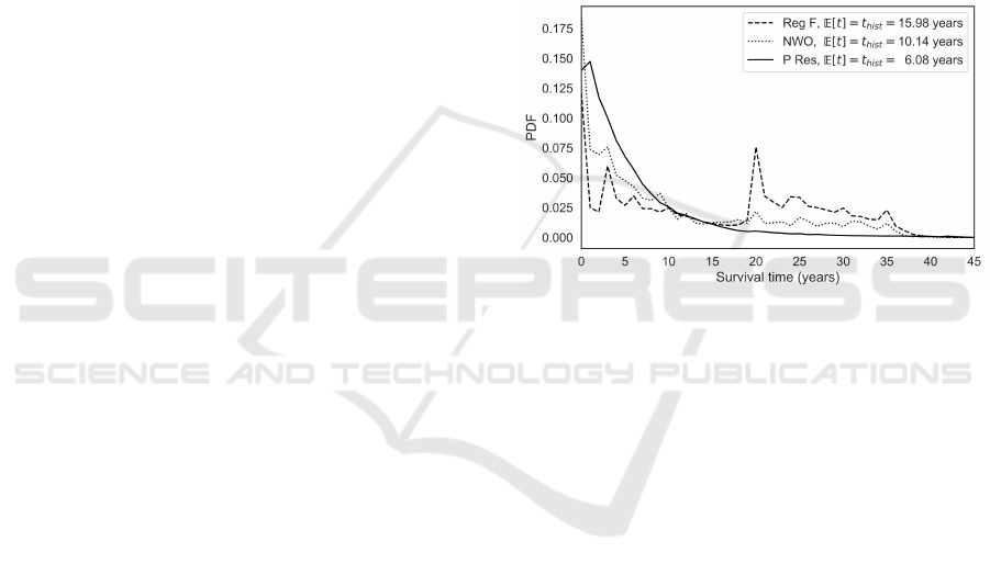
ﬂeet recapitalization (∼ 3600 observations). Figure

1 shows the probability distribution functions (PDFs)

constructed from the histograms of empirical service

lifetime data (binned annually). We determine the

average lifetime E[t] = t

hist

from the empirical his-

togram and use this to determine the effective at-

trition rate parameter α

hist

= 1/t

hist

(α

RegF

≈ 0.063,

NWO

≈ 0.099, α

PRes

≈ 0.164) (see (Bryce and Hen-

derson, 2020) for further details).

Figure 1: Empirical survival time PDFs for three CAF sub-

populations: Reg F, P Res, and NWO [Reg F].

4.1 Steady State Regime

Each population is grown from zero to a steady state

population of P

= 1000. The intake rate is constant

year over year and set to the steady state value given

by in

= αP

(E0). Intake times are uniformly dis-

tributed over the yearly interval with associated at-

trition times determined by sampling lifetimes from

the population’s survival distribution. A total simula-

tion time of 1300 years was chosen in order to give

an abundance of time for each population to reach

steady state. Recall that the e-folding time for a mem-

oryless population is given by the characteristic mean

lifetime according to e

−αt

= e

−t/E[t]

(1 e-folding time

ranges from 100 to 0.5 years for α ∈ [0.01,2.0]). Re-

fer to (Bryce and Henderson, 2020) for a discussion

on transient time to steady state for the populations

considered here.

Estimator bias was measured over each replica-

tion and for every interval during the steady state re-

gion (600 simulation years). Relative residual error

([

α −α]/α) for all simulated populations is presented

in Figure 2 (solid curves) with precision shown us-

ing the standard error of the mean (SEM) (shaded re-

ICORES 2023 - 12th International Conference on Operations Research and Enterprise Systems

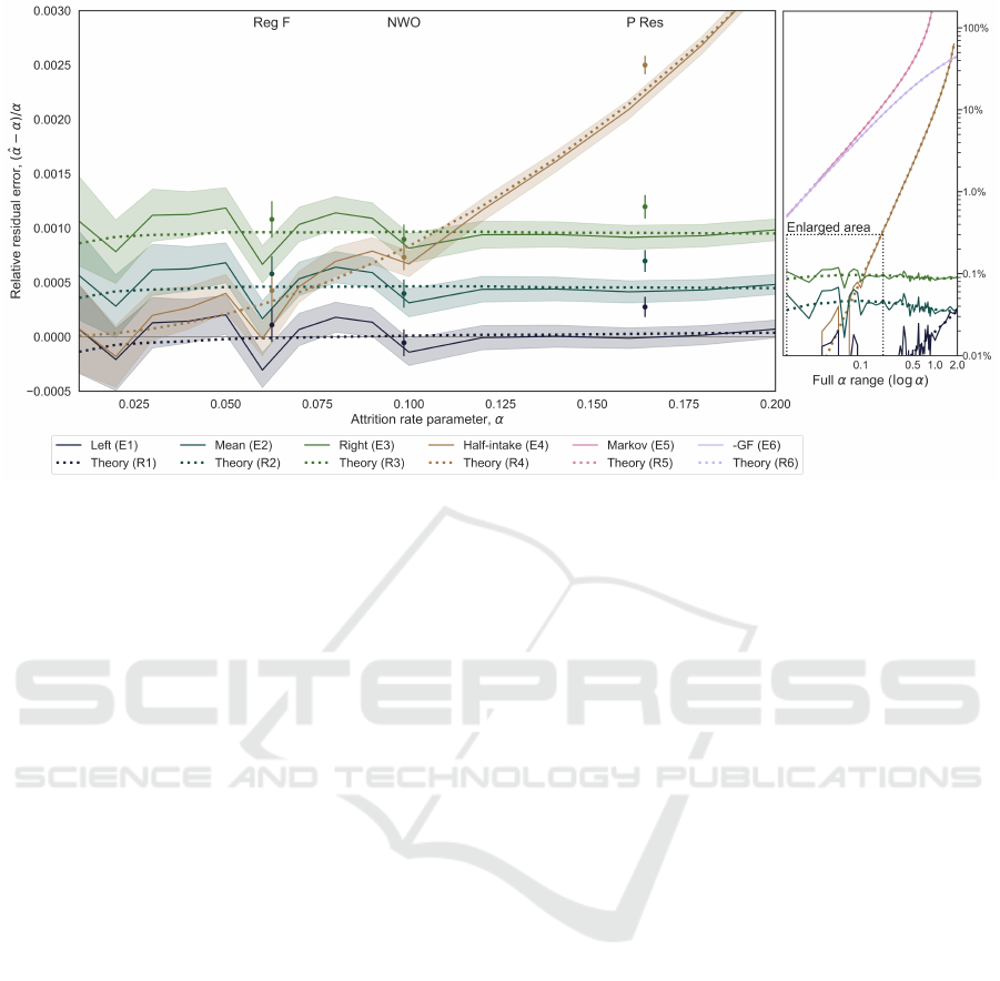
Figure 2: Attrition rate parameter estimator performance in the steady state regime. Mean relative residual error results

(solid curves) with corresponding theoretical expectation (dotted curves) are plotted against set α. The main plot (left-hand

side) focuses on the region of α ≤ 0.2. Estimator results from populations simulated using empirical survival lifetimes are

shown for comparison (points). Precision on mean results is presented as a shaded region (memoryless populations) or error

bars (empirical populations) representing ±1SEM. Results for the full parameter range (α ∈ [0.01,2.0]) are shown on the

right-hand side plot (log-log scale). Note that the negative of the GF estimator residual error (E6) is plotted here to facilitate

comparison.

gion ±1SEM). The main plot (left-hand side) focuses

on α ≤ 0.2 (i.e., often observed for real workforces)

while the right-hand side plot shows the full experi-

mental results over a larger range of relative residual

error (up to ∼ 100%). To aid in the visualization, at

an attrition rate set to α = 0.1, the measured mean

estimators results in the following order from small-

est (lowest curve) to largest (highest curve) resid-

ual error: Left (E1: gray), Mean (E2: blue), Right

(E3: green), Half-intake (E4: brown), General For-

mula (E6: violet, note that the negative residual er-

ror is plotted here for ease of comparison, see Section

3.2.2), and Markov discrete (E5: pink).

Performance results for the empirical populations

(points with error bars ±1SEM) were determined by

comparing the measured mean estimator against α

hist

(recall Section 4 and Figure 1).

4.2 Dynamic Regime

The population set that should capture most work-

force situations, α ∈ [0.1,0.5], was chosen as a rep-

resentative sample to examine estimator performance

during population growth and reduction scenarios. In

this experiment, populations are grown with a con-

stant intake rate of in = 100/year from zero to a

steady state population of P

= in/α. A growth mul-

tiplier, δ ∈ [0, 2], is then applied to the intake, caus-

ing a step change in the rate. Note that δ = 0 cor-

responds to a free fall in population (i.e., no intake),

δ = 1 corresponds to the steady state, and δ = 2 will

lead to a doubling of the intake rate (and eventual dou-

bling of the population). Due to computational time

constraints, the total simulation time varies with each

population in order to allow enough time to reach

steady state.

The ﬁrst time interval after δ is applied, t

, corre-

sponds to the greatest population change that occurs

during the dynamical regime (see Equation 2). For

this reason it is in the ﬁrst interval that we compare

attrition estimator performance. As in the steady state

experiment, the residual error between the mean esti-

mator

α and the set α is used as an indicator of per-

formance. The relative error ([

α −α]/α) for each es-

timator at t

are shown against δ as a heat map in Fig-

ure 3 using a restricted scale from −0.2 (dark blue)

to 0.2 (dark red). We cut off at a relative error of

0.2 (i.e., 20%), as the Markov (E5) and General For-

mula (E6) range is large enough (−0.21,0.86) that we

lose visual distinction for the other estimators other-

wise. The growth multiplier δ = 1 case corresponds to

the steady state case (dotted boxes) and results match

those in Section 4.1 and Figure 2.

Estimating Workforce Attrition Rate Parameters: A Controlled Comparison

Figure 3: Attrition rate parameter estimator performance during dynamic population change. Relative mean residual error

results are shown as heat maps for each estimator using a scale of −0.2 (dark blue) to 0.2 (dark red); we cut off at a relative

error of 20% , otherwise we lose visual distinction since the E5 and E6 range is very large. Estimators are measured over the

interval immediately after growth (δ > 1) or decay (δ < 1) is initiated in order to examine the maximum effect. The δ = 1

corresponds to the steady state (dashed box) and results here follow those in Figure 2.

5 DISCUSSION

5.1 Estimator Accuracy: Steady State

As expected for memoryless populations in steady

state (Figure 2), for small α, we see all estimators con-

verging (mean relative residual error going to zero).

The log scale on the right-hand side of Figure 2 shows

relative error in % α, a gauge of the error an analyst

might expect. For common values of α (≤ 0.2), the

magnitude of the bias is very small for most estima-

tors (< 0.4% for E1 - E4) and becoming uncomfort-

ably large yet likely remaining within tolerance levels

for the remaining (∼ 12% for E5 and ∼ 9% for E6).

In all cases, results follow analytical expressions

for residual error of the estimators (Equations R1–

R3, R4–R6, dotted curves in Figure 2), with a few

interesting features. At lower α (< 0.15) there is

an apparent cyclic pattern that diverges from the an-

alytically derived residual, with a magnitude of or-

der 0.0001. We attribute this to ﬁnite sample error

and happenstance (spurious pattern); which we con-

ICORES 2023 - 12th International Conference on Operations Research and Enterprise Systems

ﬁrmed by running additional trials and ﬁnding larger

error than implied by the SEM. This can be under-

stood as, for correlated data, the effective sample size

is smaller than the sample size of 1000 replications

x 600 years for our experiments. As the correlation

length is related to the e-folding time we have an ef-

fective SEM

e f f

∼ SEM/

√

α and we see a rapid in-

crease in variation as α decreases.

Figure 4: Mean relative residual error (E1–E3, steady state).

Additionally, as α gets larger the error on E1 in-

creases and approaches E2. This is highlighted in Fig-

ure 4 where we conﬁrm that the relationship between

the three continuous estimators deﬁned by Equation

10 holds in expectation for all α considered (i.e., re-

arrangement of (10) gives E[α

] = 2E[(α

)/(α

)], red dotted curve).

As for the populations with empirical distributions

(Figure 1) the mean relative residual error shows a

small positive bias with respect to the memoryless

model (see points with error bars in Figure 2, which

lie above the theoretical relative residual). Part of this

difference can be explained by considering that, un-

like the memoryless populations, the empirical sur-

vival distributions do not have a tail beyond a deﬁned

cut-toff lifetime, T . Take, for example, the NWO sur-

vival PDF reproduced in Figure 5.

Figure 5: Empirical survival PDF and mean relative residual

error of E1 for NWO in steady state.

Visually, the survival time PDF of NWO’s shape

lies between the other two sub-populations, with an

initial spike at small lifetimes and the tail cut off at

T = 41 (Figure 1). The left-hand side of Figure 5

shows the survival PDF (ﬁlled area) along with sev-

eral exponential ﬁts: an exponential with α = 1/t

hist

(black curve), and two truncated exponentials cut off

at T = 40 (red dotted curve) and T = 50 (blue dot-

ted curve) with attrition rate parameter α

∗

such that

E[t] = t

hist

. The right-hand side of Figure 5 shows

the corresponding steady state results for the empir-

ical PDF (black point), and the T = 40 and T = 50

truncated exponentials (red and blue points, respec-

tively). These results illustrate the sensitivity to the

tail of the distribution. By implication there is sen-

sitivity to the speciﬁcs of the distributions shape, as

might be expected. However, we see the absolute er-

ror is small and would be well below stochastic mea-

surement error (e.g., in a population of 10,000 or less

a difference of a few individuals attriting introduces

as large or larger error to the measured α) indicating

that, at least near steady state, the memoryless estima-

tors and model can be expected to perform well and

the memoryless assumption is well speciﬁed. Similar

results were found for both Reg F and P Res.

5.2 Estimator Accuracy: Dynamics

Often for institutional planning, a population in

steady state is an aspiration rather than a reality. A

good method for measuring the attrition rate parame-

ter will likely differ when said population is in equi-

librium (Figure 2) and when undergoing changes in

intake (Figure 3).

In periods of growth (right-hand side of Figure 3

panels), P

is less than P

with the difference between

them increasing with inﬂow (δ) and decreasing with

outﬂow (α). Conversely, in periods of decline (left-

hand side of Figure 3 panels) P

is greater than P

with the difference between them increasing with de-

creasing α and δ.

While E1 performed the best in steady state (Fig-

ure 2, dashed box at δ = 1 in Figure 3), it’s depen-

dence on P

in the denominator guarantees positive

bias during growth (red shade) and negative bias dur-

ing decline (blue shade). The behaviour of E3 mir-

rors that of E1, though with opposite bias consider-

ing it’s denominator is P

. Conversely, both E2 and

E4 perform very well during periods of ﬂux since

their formulations consider changes in P (mean P and

+ in/2, respectively). The discrete estimators (E4-

E6) all perform well in free fall (δ = 0), as expected

as they are correctly speciﬁed in this case, but error

accrues as intake and outﬂow increase. E6 retains it’s

negative bias.

As with the steady state results, the empirical

populations in growth and decline vary from the

behaviour set by the memoryless populations, with

NWO and Reg F standing out in particular in Figure

Estimating Workforce Attrition Rate Parameters: A Controlled Comparison

3. This illustrates the sensitivity of the estimators to

the shape of the survival distributions (Figure 1). Sim-

ilarly to the steady state, the truncated exponential ﬁts

to the empirical histograms more closely follow the

memoryless results (see Figure 5 for the NWO case).

5.3 General Formula

We have empirically measured the single interval

GF here, but note that the multi-interval GF (Equa-

tion GF) can be derived from the ODE describing a

memoryless population. To do so we consider regions

deﬁned by intake events, where E6 gives the estimate

on the i-th interval

= 1 −

+ out

, (14)

where we drop the hat for convenience and use i as the

index. Using γ

= 1 −e

−α

, with t

being the length

of the i-th interval we have

−α

+ out

, (15)

and we take the natural logarithm of both sides

−α



+ out



. (16)

We then ﬁnd the average α over the N sub-intervals

−α =

∑

i=1

−α

∑

i=1



+ out



. (17)

We will be generalizing the GF by keeping the t

’s in,

but note for equal (constant) t

and when measuring

on a unit interval we can pull t

out of the sum and

= 1, making the time units implicit. To facilitate

generalizing the GF we recast the equation as

−α =

∑

i=1



+ out



, (18)

and we apply the exponential function to both sides

−α

= e

∑

i=1



+out



∏

i=1



+out



. (19)

The exponential and natural logarithm cancel each

other out, and if we measure over the unit interval we

will have γ = 1 −e

−α

leading to

1 −γ =

∏

i=1



+ out



(20)

which we call the “Generalized General Formula”, as

it explicitly takes into account differing sub-interval

sizes. Note that for equal t

on the unit interval Nt

= 1

and we recover the GF.

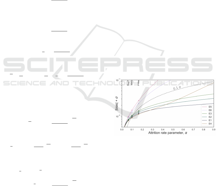
5.4 Estimator Choice

When confronted with annual data we have to con-

sider both the accuracy (bias) and precision (varia-

tion) of the estimators. As a simple performance

measure we consider the error envelope of the bias

plus standard deviation, as an estimate of measure-

ment error. In Figure 6 we see that the continuous es-

timators, and the half-intake estimator, perform best

with about 10% expected measurement error (dot-

ted line). We attribute the half-intake’s good per-

formance to the stabilizing effect of including intake

(ﬁxed value). Notably, we can ﬁnd an equivalent half-

intake formula from Equation 6 using Taylor expan-

sions, with the identical form but which directly es-

timates α. The performance of this direct half-intake

estimator is worse than the classic half-intake. This

shows sensitivity to the speciﬁc uncontrolled approx-

imations made, and difﬁculty in reasoning about per-

formance.

Overall, the Mean estimator (E2) is the best choice

for attrition rate parameter considering both it’s per-

formance (closely following the Left estimator [E1]

in steady state [Figure 2] and having the best per-

formance [i.e., least bias] during dynamic population

change [Figure 3]) and it’s simplicity. The half-intake

estimator, which bridges the continuous-discrete di-

vide as it is a partial correction, is the best performing

estimator at low to moderate attrition.

Figure 6: Performance measure of estimator bias + σ in

steady state.

It should be noted that use of the mean population

estimator is standard practice for measuring employee

turnover (i.e., attrition). For example, the U.S. De-

partment of Labor (U.S. Bureau of Labor Statistics,

2022) deﬁnes employee turnover as the number of

employees who leave divided by the average number

of employees. Additionally note that, constrained to

measuring at a constant frequency over a unit time in-

terval such that dt = (1/N), that

t+1

Pdt = dt

∑

P =

(1/N)

∑

P while

P = (1/N)

∑

P and taking the aver-

age

P is identical to integrating the population over

ICORES 2023 - 12th International Conference on Operations Research and Enterprise Systems

the interval and so the mean average estimator (E2)

recovers the exact estimator (Equation 8). While all

estimators converge in the limit of diminishing mea-

surement intervals the fact that the average is ro-

bust on large (e.g., annual) intervals, has limited bias,

matches common labour practice, is used by multiple

militaries, and has a particularly simple connection to

the exact estimator recommends its use.

6 CONCLUSION

We show that the continuous model of attrition leads

to marginal, but real, improvements over the discrete

Markov chain view that has dominated for over three

quarters of a century (Seal, 1945). We provide in-

sight into three important aspects: 1) we conclusively

demonstrate which common estimators work best in

practical situations (the two-point average population

and half-intake estimators), 2) we ﬁnd the theoreti-

cally exact estimator and demonstrate all common es-

timators are approximate solutions to this exact esti-

mator, and 3) we derive the analytical residuals for

common estimators which provides an understanding

of their bias properties.

REFERENCES

Anderson, T. W. and Goodman, L. A. (1957). Statistical

inference about Markov chains. The annals of mathe-

matical statistics, pages 89–110.

Bartholomew, D. and Forbes, A. (1979). Statistical Tech-

niques for Manpower Planning. John Wiley.

Bryce, R. M. and Henderson, J. A. (2020). Workforce

populations: Empirical versus Markovian dynamics.

In 2020 Winter Simulation Conference (WSC), pages

1983–1993. IEEE.

Devroye, L. (1998). Non-Uniform Random Variate Gener-

ation. Springer, London, 2nd edition.

Feller, W. (1957). An Introduction to Probability Theory

and Its Applications, volume 1 & 2. John Wiley &

Sons, Inc.

Henderson, J. A. and Bryce, R. M. (2019). Veriﬁcation

methodology for Discrete Event Simulation models of

personnel in the Canadian Armed Forces. In 2019

Winter Simulation Conference (WSC), pages 2479–

2490. IEEE.

Higham, N. J. (2008). Functions of Matrices: Theory and

Computation. SIAM.

Merck, J. W. and Hall, K. (1971). A Markovian ﬂow model:

The analysis of movement in large-scale (military)

personnel systems. Technical report, RAND CORP

SANTA MONICA CALIF.

Okazawa, S. (2007). Measuring attrition rates and fore-

casting attrition volume. Technical Report DRDC

CORA TM 2007-02, Defence Research and Develop-

ment Canada.

Seal, H. (1945). The mathematics of a population com-

posed of k strata each recruited from the stratum be-

low and supported at the lowest level by a uniform an-

nual number of entrants. Biometrika, 33(3):226–230.

U.S. Bureau of Labor Statistics (2022). Job openings and la-

bor turnover - September 2022. https://www.bls.gov/

news.release/pdf/jolts.pdf. Accessed: 2022-11-14.

Vajda, S. (1978). Mathematics of Manpower Planning. Wi-

ley.

Vincent, E. (2019). The mathematical formalism of growth

and discount rate reporting. http://www.corsottawa.

org/CORS2019.pdf. Accessed: 2022-11-14.

Vincent, E., Calitoiu, D., and Ueno, R. (2018). Person-

nel attrition rate reporting. Technical Report DRDC-

RDDC-2018-R238, Defence Research and Develop-

ment Canada.

Vincent, E., Okazawa, S., and Calitoiu, D. (2021). Attrition,

promotion, transfer: Reporting rates in personnel op-

erations research. In ICORES, pages 115–122.

Young, A. and Almond, G. (1961). Predicting distributions

of staff. The Computer Journal, 3(4):246–250.

Estimating Workforce Attrition Rate Parameters: A Controlled Comparison