A Low-Cost Sensors Study Measuring Exposure to Particulate

Matter in Mobility Situations

Marie-Laure Aix

, Mélaine Claitte and Dominique J. Bicout

Univ. Grenoble Alpes, CNRS, UMR 5525, VetAgro Sup, Grenoble INP, TIMC, 38000 Grenoble, France

Keywords: Low-Cost Sensor, PM

2.5

, Calibration, Mobility, Exposure Assessment.

Abstract: In 2013, the International Agency for Research on Cancer classified particulate matter (PM) as carcinogenic

to humans. It is therefore essential to measure PM concentrations to minimize the exposure of individuals.

Our objective was to investigate personal exposure to PM

2.5

(PM with diameter ≤ 2.5 µm) in Grenoble

(France) during commuting in different transportation modes: bike, walk, bus and tramway. PM

2.5

measurements were found to be the highest for bikes, followed by walk, bus, and tramway. In this study,

conducted in spring during low pollution levels of PM, exposure levels are greatly influenced by the time of

day. Pedestrian and cyclists’ exposure generally stayed under background reference values. Exposure in

public transportation was usually below reference values, but when background PM

2.5

levels went lower

(evening), levels registered in the tramway or bus reached those of the reference. Therefore, public transport

users could be less exposed than active commuters, except when ambient pollutant levels are low.

Environmental parameters like wind might be important in Grenoble, and it would be worthwhile to reproduce

this study at a time when wind speed is lower.

1 INTRODUCTION

Every year, it is estimated that outdoor air pollution

causes 7 million deaths around the world (Fuller et

al., 2022). Particulate matter (PM) is made of solid

compounds suspended in the air that are small enough

to be inhaled. Considered as the most dangerous form

of air pollution, PM can enter blood circulation, and

accumulate in numerous organs (Pryor, Cowley, &

Simonds, 2022). Therefore, it is important to assess

populations’ exposure to PM, which is generally done

by official reference monitoring stations. However,

more and more scientists state that stationary

monitoring stations are not always representative of

people’s exposure (Van den Bossche et al., 2015; F.

Yang et al., 2019). This might be related to the time

that people spend indoor and outdoor, in places where

the pollutant levels do not always equal to reference

values. Time spent in transportation could represent

up to 30% of the inhaled dose (Dons, Int Panis, Van

Poppel, Theunis, & Wets, 2012). According to Han et

al. (2021), personal exposure to PM

2.5

(PM with

diameter ≤ 2.5 µm) measured by portable sensors, is

https://orcid.org/0000-0001-5366-2372

https://orcid.org/0000-0003-0750-997X

significantly associated with an increase in

respiratory and systemic inflammatory biomarkers.

However, the associations are weaker when ambient

2.5

concentrations, measured by fixed reference

stations, are used as an exposure proxy. Low-cost

sensors demonstrate good accuracy to measure

individual exposure to PM (Motlagh et al., 2021) and

can therefore be used for exposure studies, especially

during commuting. Few mobility studies involving

low-cost sensors have been performed, especially in

low-concentration situations. Many surveys take

place in Asia where pollution levels are usually

higher than in Europe. During 10 working days, we

conducted a field experiment to collect PM

measurements using four transportation modes

around Grenoble (France): bike, walk, bus, and

tramway. Our objective was to estimate personal

exposures to PM

2.5

with a low-cost sensor during

commuting in different modes. Another purpose was

to compare the so measured concentrations with

reference values. We wanted to know whether the

low-cost sensors could be used to assess differences

between transport modes and the time of day. In

Aix, M., Claitte, M. and Bicout, D.

A Low-Cost Sensors Study Measuring Exposure to Particulate Matter in Mobility Situations.

DOI: 10.5220/0011747600003399

In Proceedings of the 12th International Conference on Sensor Networks (SENSORNETS 2023), pages 32-41

ISBN: 978-989-758-635-4; ISSN: 2184-4380

 2023 by SCITEPRESS – Science and Technology Publications, Lda. Under CC license (CC BY-NC-ND 4.0)

doing this, we hope to contribute to the exposure

literature using low-cost sensors.

2 MATERIALS AND METHODS

2.1 Particulate Matter Sensor

2.1.1 Monitoring Devices

PM concentrations were measured using two

AirBeam2 (HabitatMap), which entail an optical

sensor (Plantower PMS7003). AirBeam2 are

inexpensive ($249) and measure concentrations of

, PM

2.5

, PM

, temperature and relative humidity

(RH). They are connected to a smartphone via

Bluetooth and provide real time values to users. With

the growth of the Internet of Things (IoT) sector (Das,

Ghosh, Chatterjee, & De, 2022; Y. Yang et al., 2022),

cheaper PM sensors are currently available on the

market. However, they often have to be assembled

with other components like microcontrollers or GPS

modules, and an IoT platform has to be set-up for data

visualisation. Designing a monitoring station,

assembling components and developing a data

visualisation tool are different steps which can be

time-consuming. HabitatMap already provides an

online platform (http://aircasting.org) for viewing and

downloading AirBeam2 data. Furthermore,

AirBeam2 are ready-to-use devices. South Coast Air

Quality Management District (2018) compared the

AirBeam2 PM

2.5

measurements to values given by

three Federal Equivalent Method instruments. They

observed very strong correlations in the laboratory

studies (R

> 0.99) and moderate to strong

correlations with different reference instruments from

the field (0.68 < R

< 0.79). More recently, Tong, Shi,

Shi, and Zhang (2022) found that Airbeam2

measurements correlated well with roadside official

monitoring stations. They also reported a good

agreement (R

= 0.67–0.89) between Airbeam2 local

measurements and the predictions from a model

involving satellite observations. AirBeam2 is already

calibrated by the manufacturer, but the calibration

equations do not account for RH (HabitatMap, 2022).

Huang et al. (2022) found that the accuracy and bias

of the PM data reported by AirBeam2 sensors were

affected by rainy weather and high humidity

environments. Moreover, Zou, Clark, and May

(2021) suggested that there was a significant linear

relationship between RH and the relative response of

the low-cost PM sensors to the research-grade

instruments. Therefore, we calibrated the devices by

accounting for RH.

2.1.2 Calibration

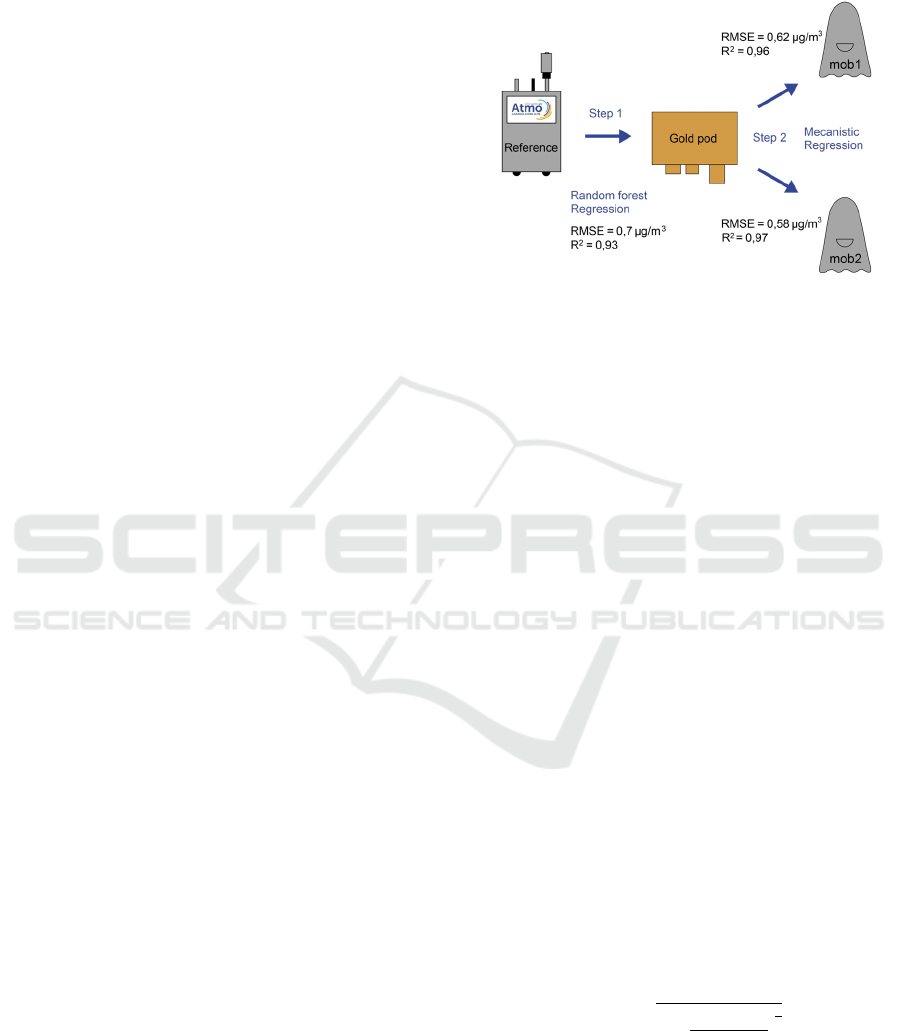
The calibration process involved two steps (Figure 1).

Figure 1: Two steps calibration process.

• Step 1: Calibration of a Fixed Low-Cost

Sensor (“Gold Pod”) with a Reference Device

Before this study, we had already calibrated a low-

cost fixed station by collocating it with a Palas GmbH

200 (Reference) from Atmo Auvergne-Rhône-Alpes

(Atmo AuRA) in Grenoble “Les Frênes” (Refer

Figure 4). This calibration was performed using a

random forest regression technique developed by

Schmitz et al. (2021) comparing this individual fixed

sensor with the reference station. This low-cost fixed

station, called “gold pod” used the same optical

sensor (PMS7003) than the mobile devices.

• Step 2: AirBeam2 Sensors Calibration with a

Fixed Low-Cost sensor (“gold Pod”)

Next, 44 days of calibration were performed from

September 20, 2022 to November 3, 2022 where the

two AirBeam2 were collocated close to the “gold

pod”. The two mobile devices were calibrated

independently: first, the AirBeam2 used by

experimenter 1 (“mob1”) and then the device used by

experimenter 2 (“mob2”). This was motivated by the

observation that mob2 was delivering concentrations

a bit higher than mob1. By using the nls() function

from RStudio 2022.07.1 (R Core Team, 2022) on

75% of the dataset, we applied the mechanistic

equation (Equation 1) involving relative humidity and

temperature for calibration:

ଶ.ହ ୥୮

ൌ a ൅b

୔୑

మ.ఱ ౣ౥ౘ

൬

ଵାୢ

౎ౄ

ౣ౥ౘ

భబబష౎ౄ

ౣ౥ౘ

൰

భ

య

൅c T

୫୭ୠ

(1)

where PM

2.5 gp

= PM

2.5

concentrations in µg/m

given

by the “gold pod”, PM

2.5 mob

= PM

2.5

concentrations

(µg/m

) measured with the AirBeam2, RH

mob

relative humidity in % determined by the AirBeam2,

mob

= temperature in °C given by the AirBeam2. For

A Low-Cost Sensors Study Measuring Exposure to Particulate Matter in Mobility Situations

mob1, we found a = 0.49, b = 0.91, c = 0.07 and d =

0.43. For mob2, we had a = -0.1, b = 0.86, c = 0.08

and d = 0.31. We then tested these two calibration

formulas on the remaining 25% dataset, and we found

the following performance indicators. For mob1, we

had RMSE = 0.62 µg/m

and R

= 0.96 and for mob2,

we found RMSE = 0.58 µg/m

and R

= 0.97. RMSE

(root mean square error) reflects the accuracy of the

model to predict actual PM

2.5

values, and R

(coefficient of determination) refers to the correlation

between the AirBeam2 values and the reference

concentrations. Based on this, we decided to continue

with these models as the indicators were good

compared to what is found in the literature (Blanco et

al., 2022; Haghbayan & Tashayo, 2021).

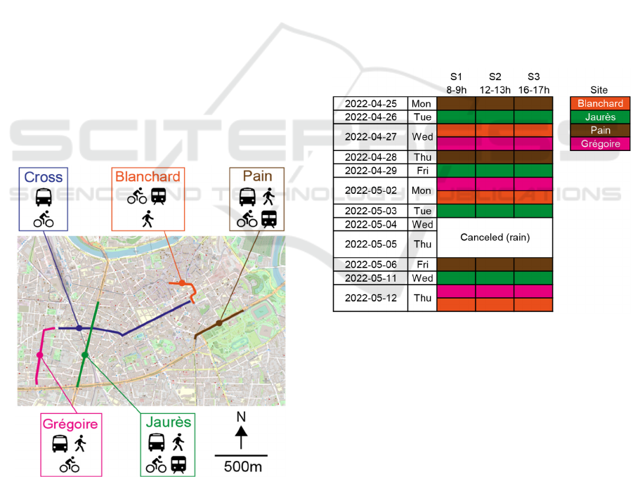
2.2 Sampling Design

2.2.1 Monitoring Routes

The study took place in Grenoble, the largest city in

the Alps, hosting around 450,000 inhabitants. Five

different monitoring sites were selected (Figure 2):

two wide streets (“Jaurès” and “Pain”) and two

narrow (also called “canyon”) streets surrounded by

higher buildings (“Grégoire” and “Blanchard”). We

also monitored PM when we commuted between

Blanchard and Grégoire (“Cross” route).

Figure 2: Monitoring routes used in the experiment.

Credits: © OpenStreetMap contributors.

2.2.2 Experimental Timings

Ground measurements were conducted from April 25,

2022 to May 12, 2022 during 10 working days

(Figure 3). Three different measurement sessions

were performed daily: a first session (S1, morning)

between 8:00 and 9:00, a second session (S2,

noontime) between 12:00 and 13:00 and a third

session (S3, afternoon) between 16:00 and 17:00.

Sometimes, for reasons related to the public transport

timetables, the sessions went slightly beyond the time

slots. Nine sessions were postponed because of rainy

conditions.

Two experimenters were involved in the study.

For each session, they had to travel the same routes in

parallel using different modes of transport: bike,

walk, bus or tramway (Appendix). Each site was

sampled for at least three days (Figure 3). On the days

when we studied Blanchard and Grégoire, we also

monitored PM while travelling in between the two

sites (“Cross” route). Jaurès was sampled four times

because this street, longer than the others, had many

potential biases (intersections, stores, idling cars) and

we thought it might be interesting to replicate the

measurements further.

Figure 3: Measurement campaign schedule.

Next, we analysed carefully the public transportation

schedules. A session example is reported in the

Appendix. The same document was used as a

roadmap by the experimenters for each session.

Reproducing measurements on the same street is

important to be representative (Van den Bossche et

al., 2015). Every day, each experimenter performed

at least 12 repetitions of the route.

2.3 Data Cleaning

In this paper, we decided to focus only on PM

2.5

analysis and on commuting times. We left PM

, PM

and results related to waiting times for further work.

SENSORNETS 2023 - 12th International Conference on Sensor Networks

Data were extracted via AirCasting application and

analysed with RStudio. We retrieved 214 comparison

trips where the two experimenters were travelling

along the same routes (428 trips in total, considering

both experimenters). PM sensors can be vulnerable to

inaccuracies resulting from drift, temperature,

humidity and other factors (Motlagh et al., 2021). As

both AirBeam2 were quite new, drift was not an issue,

but we blew compressed air through the intake of the

gold pod used for calibration as recommended by

Bathory, Dobo, Garami, Palotas, and Toth (2021). As

explained above, both AirBeam2 devices were

calibrated using formulas accounting for RH and

temperature. We also checked the presence of dust

with CAMS (Copernicus Atmosphere Monitoring

Service) satellite data (retrieved 0.1° x 0.1° resolution

dust values from ENSEMBLE dataset (METEO

FRANCE, 2020) (‘analysis’ type)). Fortunately, no

dust event happened during the experiment period.

We removed outliers in the dataset because we had

peak events on trips, even inside public transports,

mainly because of smokers or idling cars. In public

transports, those peaks were often caused by door

openings. All outliers with more than 1.5 times the

interquartile range above the third quartile (Q3) or

less than 1.5 times the interquartile range below the

first quartile (Q1) were removed. Hourly background

reference PM

2.5

concentrations from Atmo AuRA

were collected through their Application

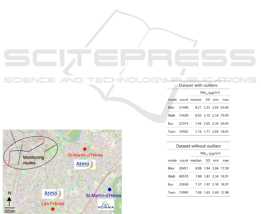
Programming Interface (https://api.atmo-aura.fr/).

For this study, we used the average from two

background reference stations (Les Frênes and Saint-

Martin d’Hères). Both references, placed at

approximately 3 km from the experimental sites, were

located in relatively open areas (Figure 4). For each

measurement made every second with our mobile

devices, we affected the corresponding hourly value

Figure 4: Location of the Atmo AuRA reference stations (in

red) and ROMMA meteorological station (in blue). Credits:

given by the reference stations. We also used

meteorological data from the Réseau d’Observation

Météo du Massif Alpin (ROMMA, 2022). Their

nearest weather station (GPS coordinates: latitude =

45.169°, longitude = 5.768°) was located around 3 km

from the collocation site (Figure 4). A Davis Vantage

Pro2 instrument registered all weather parameters.

Wind speed (km/h) corresponded to a 10-mn average,

with a measurement frequency of 2.5-3 s. We

checked that all data sources used the same time zone

(Europe/Paris).

3 RESULTS

3.1 Descriptive Statistics

Collected PM

2.5

data are summarized in Table 1.

More measurements were performed on walking

mode because, in order to replicate the experiment

and use public transportation again, we had to walk

back to the starting point. This was especially true on

routes where public transport was only running in one

direction. The number of measurements made on foot

were also higher because walking the road segment

took longer than cycling, taking the bus or tramway.

Table 1: Descriptive statistics on PM

2.5

concentrations and

number of measurements (count) performed in different

commuting modes.

More outliers were identified for walking (5.3%) than

for cycling (4.6%), tramway (4.1%) or bus (3.1%).

Walkers are generally more exposed to PM coming

from smokers, restaurants or bakeries. In addition,

they are close to idling cars. When leaving outliers in

A Low-Cost Sensors Study Measuring Exposure to Particulate Matter in Mobility Situations

the dataset, cyclists were more exposed (median: 8.2

µg/m

) than walkers (median: 8 µg/m

), followed by

buses (median: 7.4 µg/m

) and tramway (median: 7.2

µg/m

). Compared with cyclists, pedestrians were

2.2% less exposed, bus users 9.4% less and tramway

commuters 12.8% less. When removing outliers, the

exposure ranking proved to be the same. Cyclists

were more exposed (median value of 8.1 µg/m

) than

walkers (median: 7.9 µg/m

), followed by bus users

(median: 7.4 µg/m

) and tramway (median: 7.1

µg/m

). Compared to cyclists, walkers were 2.4%

less exposed, bus commuters 8.6% less and tramway

users 12.2% less. Qiu and Cao (2020) also found that

walkers were more exposed than bus commuters.

Peng et al. (2021) and Wang et al. (2021) found the

same exposure ranking (bike>walk>bus). They used

a PMS3003 device, similar to PMS7003. According

to Shen and Gao (2019), cyclists and pedestrians can

be directly exposed to other local particle emissions

along the road, which probably results in elevated PM

concentrations in specific areas and times. In a study

taking place in Nantes (France), Muresan and

François (2018) stated that public transport users

would accumulate 4–11 times less PM in their lungs

than nearby pedestrians walking the same route. We

decided to pursue all further analyses after having

removed outliers in our dataset.

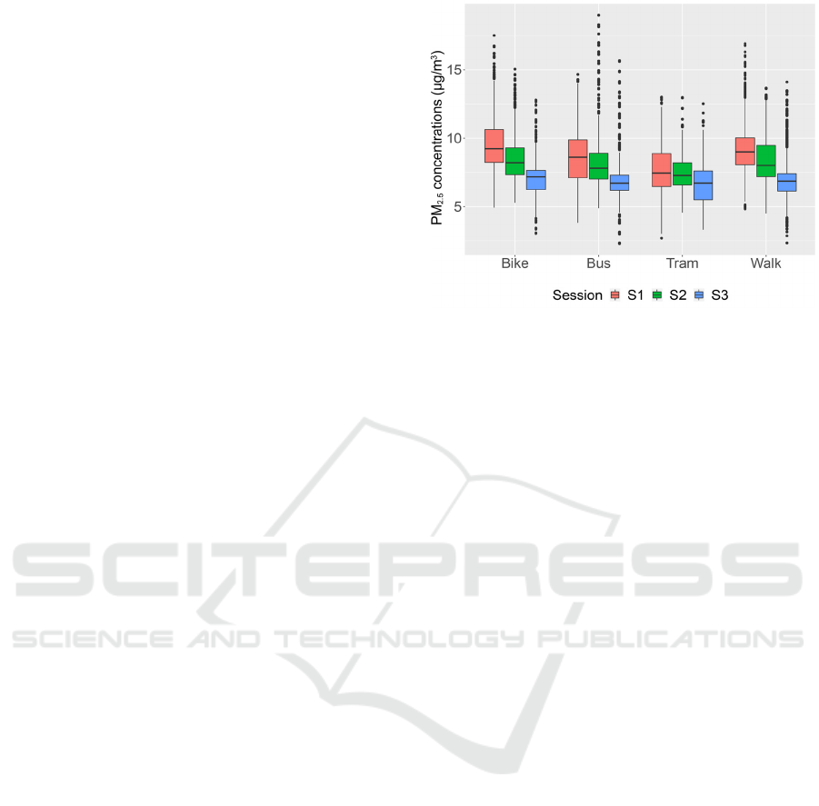
3.2 Comparison Between Travel Modes

Exposure levels are greatly influenced by the time of

day (Figure 5). The morning session (S1) showed

higher PM

2.5

concentrations, followed by the

noontime (S2) and the afternoon session (S3).

Of all transport modes combined, S1 PM

2.5

median was 12.9% higher than S2, while S2 median

was 15.3% higher than S3. In the tramway, diurnal

variations seem to be reduced compared to other

modes. deSouza, Lu, Kinney, and Zheng (2021) also

found that time of day (evening/morning) had an

influence. In their ANOVA analysis, travel mode

explained 9% of the variability in PM

2.5

concentrations

whereas time of day explained 8%

variability.

All sessions considered, cyclists are the most

exposed commuters. Abbass, Kumar, and El-Gendy

(2021) studied morning and evening PM

2.5

peaks. In

their work, daily exposure patterns when walking or

cycling looked similar, whereas microbus

concentrations behaved differently, and cycling

resulted in exposure to the highest average PM

2.5

concentrations.

Figure 5: Boxplots of PM

2.5

concentrations by

transport mode. Upper

and

lower whiskers show the

ranges of 5% to 95%, the central dark lines indicate

the median. The bars outside the box represent 1.5

times the interquartile range, and circles are outliers.

Per session, we observe the same PM

2.5

exposure

ranking (bike > walk > bus > tramway) but, during

S3, the levels measured in the bus get close to those

measured in the tramway. When PM

2.5

levels are high

(S1), the differences between the transport modes are

important, but when the levels are low, during the

afternoon (S3), the differences become less

pronounced. This suggests that when PM levels are

low, public transports no longer play a “protective”

role against PM

2.5

. In addition, relative differences

between sessions are lower in the tramway than in the

other transportation modes. This could mean that

levels in the tramway are less influenced by

background concentrations, which are higher in the

morning.

3.3 Comparison with Reference Value

One of the objectives of this study was to compare the

2.5

values measured by the mobile sensors with

those returned by the reference stations. The graph

below (Figure 6) shows PM

2.5

levels measured by the

mobile devices and the corresponding background

reference levels. The hours marked in bold are the

times when we carried out the most PM

2.5

measurements. As an example, the 10 am

measurements were those that we were unable to

perform as planned between 8 and 9 am. As this rarely

happened, we got fewer observations for those extra

hours.

In general, PM

2.5

levels given by the mobile

sensors were lower than values given by background

SENSORNETS 2023 - 12th International Conference on Sensor Networks

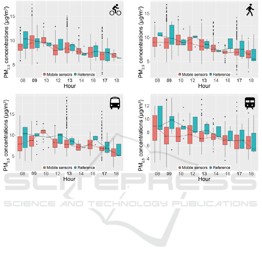
Figure 6: Comparison between values measured by mobile devices and reference values. The 9 o'clock boxplot corresponds

to the values measured by mobile sensors between 8 and 9 am. The hours in bold are the ones where we had the more

measurements taken by mobile devices.

stations, especially when considering hours when the

counts were the highest (9, 13, and 17). This could

come from microscale PM

2.5

variations, as PM

2.5

the local scale could be affected by different factors.

This was surprising that measured PM

2.5

values were

lower than reference values, because we were in a

traffic situation and the reference stations are located

in a background environment. Both reference

stations, situated in opened areas, could be exposed to

more PM

2.5

which would be covered by the dense and

high buildings of the city centre where experiments

took place. The AirBeam2 calibration could also be

an explanation. The ideal way to perform a calibration

would have been to collocate our mobile devices

directly with the reference station, without using a

gold pod as an intermediary. It is also important to

note that the calibration with the reference was

performed at an hourly scale, and we had to apply it

to values given at a fine scale (seconds). Knowing the

RMSE related to step 1 calibration (Refer Figure 1),

we could expect a maximal error of 0.7 µg/m

. The

average difference between reference and mobile

values during S1 and S2 (considering 9, 13 and 17

o’clock timings) was about 1.1 µg/m

. Therefore, the

calibration error alone could most probably not

explain the observed difference. Motlagh et al. (2021)

used low-cost sensors to measure PM

2.5

in Helsinki

and saw that roadside measurements were higher than

reference values. But during spring or summer, the

pollution levels in the train, bus or tramway were well

below the ambient reference pollution levels. They

attributed this to the fact that the transport fleet in

Helsinki was quite modern and the indoor air heavily

filtered. This should be the case for tramways in

Grenoble. However, older buses might remain in

operation, and the practice of using conditioned air

depends on the weather and the driver. It would have

been interesting to know if the air was filtered in the

different buses and trams we used. Han et al (2021)

also used low-cost sensors and observed that personal

2.5

levels were consistently lower than ambient

concentrations. The Center for Advancing Research

in Transportation Emissions, Energy, and Health

(2019) measured exposure of urban cyclists in Atlanta

(United States) with a PMS5003. They concluded that

few segments recorded air quality worse than the

A Low-Cost Sensors Study Measuring Exposure to Particulate Matter in Mobility Situations

background concentration. During most of the routes,

riders experienced a better air quality than the one

registered at the monitoring location.

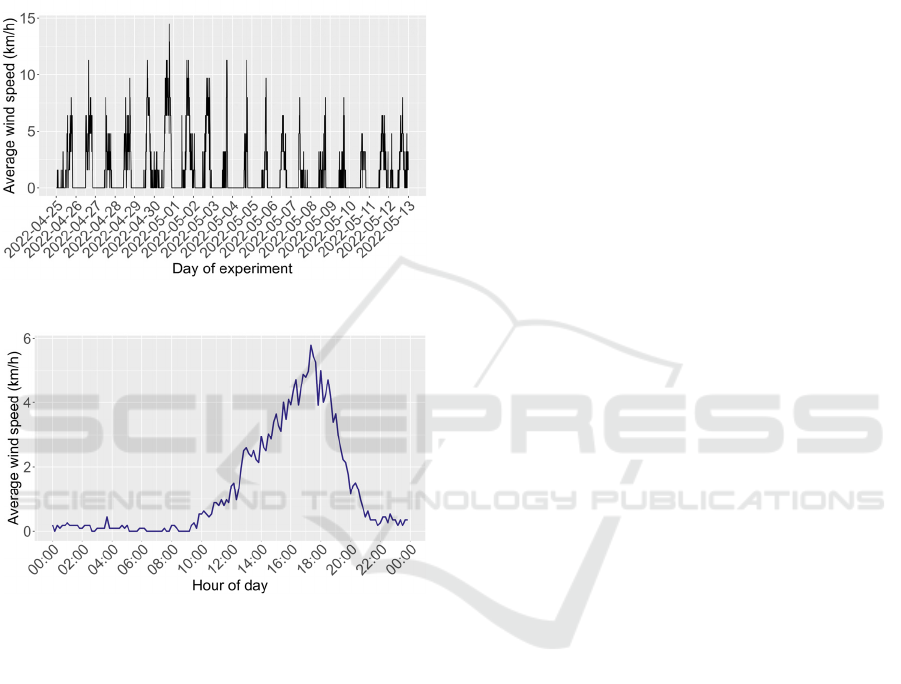
In our study, wind could be an important factor

determining PM

2.5

levels. We observed that wind

speed values were increasing starting from 10 am

(Figures 7 and 8). The relief around Grenoble could

contribute to this phenomenon.

Figure 7: Wind speed values during the experiment.

Figure 8: Average wind speed values between April 25,

2022 and May 12, 2022.

Interestingly, we observed that bus and tramway

had levels close to the reference during S3 (Refer

Figure 6). When PM levels in Grenoble were high,

public transports provided an important advantage,

but when PM levels were lower, close to their

minimum, public transportation systems did not seem

to offer this benefit any longer. Wang et al. (2021)

also performed three daily measurement sessions

(morning/noon/afternoon). Their GRIMM instrument

showed that at lower pollutant levels, the

concentrations registered in the bus were higher than

the background levels. When pollutants levels were

higher (noontime), the difference between inside and

outside got larger, as in our study. They also observed

lower levels of PM

2.5

compared to the reference when

the pollutant levels were higher. Furthermore, by

using a similar low-cost sensor (PMS3003), they

found as well that when PM

2.5

levels were lower, the

difference between reference levels and bus carriage

levels was lower.

4 CONCLUSIONS

During this spring experiment, performed in 2022 at

low pollutant levels, cyclists were more exposed than

pedestrians, bus users and tramway commuters. This

ranking was the same whether we removed outliers or

not. We counted more outliers for walking than for

cycling, tramway or bus.

When comparing exposure values to reference

stations measurements: (1) pedestrian and cyclists’

exposure generally stayed under background values,

(2) public transportation systems were under

reference values at 9 or 13 o’clock but when PM

levels went lower, levels reached those of the

reference value. Public transport users could be less

exposed than commuters using active modes, except

when ambient PM levels are low.

The time of day seems to influence exposure more

than mode of transport, with a gradual concentration

decrease throughout the day. Environmental

parameters like wind might play a role in Grenoble. It

would be interesting to reproduce this work during

another season when wind speed is lower.

In the future, we will perform an inhalation dose

calculation on the same dataset in order to consider

breathing rate differences among commuting modes.

In Grenoble, about 15% of the working population

cycles to work (Agence de la Transition Écologique,

2015), which makes the problem of PM exposure

more acute. However, we must emphasize that

cycling helps prevent many chronic diseases and

brings environmental benefits.

REFERENCES

Abbass, R. A., Kumar, P., & El-Gendy, A. (2021). Fine

particulate matter exposure in four transport modes of

Greater Cairo. Science of The Total Environment, 791,

148104. doi:10.1016/j.scitotenv.2021.148104

Agence de la Transition Écologique. (2015). La mobilité

durable de Grenoble Alpes Métropole. Retrieved from

https://territoireengagetransitionecologique.ademe.fr/

metropole-de-grenoble-met-en-place-un-systeme-de-

mobilite-durable-1-2-2/

Bathory, C., Dobo, Z., Garami, A., Palotas, A., & Toth, P.

(2021). Low-cost monitoring of atmospheric PM-

development and testing. Journal of Environmental

SENSORNETS 2023 - 12th International Conference on Sensor Networks

Management, 304, 114158. doi:https://doi.org/10.1016/

j.jenvman.2021.114158

Blanco, M. N., Gassett, A., Gould, T., Doubleday, A.,

Slager, D. L., Austin, E., Sheppard, L. (2022).

Characterization of Annual Average Traffic-Related

Air Pollution Concentrations in the Greater Seattle Area

from a Year-Long Mobile Monitoring Campaign.

Environmental Science & Technology, 56(16), 11460-

11472. doi:10.1021/acs.est.2c01077

Center for Advancing Research in Transportation

Emissions, Energy, and Health. (2019). Measuring

Temporal and Spatial Exposure of Urban Cyclists to

Air Pollutants Using an Instrumented Bike (Report No.

GT-01-09). Retrieved from https://rosap.ntl.bts.gov/

view/dot/56809

Das, P., Ghosh, S., Chatterjee, S., & De, S. (2022). A Low

Cost Outdoor Air Pollution Monitoring Device With

Power Controlled Built-In PM Sensor. IEEE Sensors

Journal, 22(13), 13682-13695. doi:10.1109/jsen.

2022.3175821

deSouza, P., Lu, R., Kinney, P., & Zheng, S. (2021).

Exposures to multiple air pollutants while commuting:

Evidence from Zhengzhou, China. Atmospheric

Environment, 247, 118168. doi:10.1016/j.atmosenv.

2020.118168

Dons, E., Int Panis, L., Van Poppel, M., Theunis, J., &

Wets, G. (2012). Personal exposure to Black Carbon in

transport microenvironments. Atmospheric Environ-

ment, 55, 392-398. doi:10.1016/j.atmosenv.2012.

03.020

Fuller, R., Landrigan, P. J., Balakrishnan, K., Bathan, G.,

Bose-O'Reilly, S., Brauer, M., Yan, C. (2022).

Pollution and health: a progress update. The Lancet

Planetary Health, 6(6), e535–e547. doi: https://

doi.org/10.1016/S2542-5196(22)00090-0

HabitatMap. (2022). AirBeam3 Technical Specifications,

Operation & Performance. Retrieved from https://

www.habitatmap.org/blog/airbeam3-technical-specifi

cations-operation-performance

Haghbayan, S., & Tashayo, B. (2021). Integrating ground-

based air quality monitoring stations with mobile sensor

units to improve the accuracy of PM

2.5

concentration

modeling. Scientific - Research Quarterly of

Geographical Data (SEPEHR), 29(116), 45-58.

doi:10.22131/sepehr.2021.242859

Han, Y., Chatzidiakou, L., Yan, L., Chen, W., Zhang, H.,

Krause, A., . . . Kelly, F. J. (2021). Difference in

ambient-personal exposure to PM

2.5

and its

inflammatory effect in local residents in urban and peri-

urban Beijing, China: results of the AIRLESS project.

Faraday Discussions, 226, 569-583. doi:10.1039

/d0fd00097c

Huang, J., Kwan, M. P., Cai, J., Song, W., Yu, C., Kan, Z.,

& Yim, S. H. (2022). Field Evaluation and Calibration

of Low-Cost Air Pollution Sensors for Environmental

Exposure Research. Sensors (Basel), 22(6), 2381. doi:

https://doi.org/10.3390/s22062381

METEO FRANCE, Institut National de l'Environnement

Industriel et des Risques (Ineris), Aarhus University,

Norwegian Meteorological Institute (MET Norway),

Jülich Institut für Energie- und Klimaforschung (IEK),

Institute of Environmental Protection – National

Research Institute (IEP-NRI), Koninklijk Nederlands

Meteorologisch Instituut (KNMI), Nederlandse

Organisatie voor toegepast-natuurwetenschappelijk

onderzoek (TNO), Swedish Meteorological and

Hydrological Institute (SMHI), Finnish Meteorological

Institute (FMI). (2020). CAMS European air quality

forecasts, ENSEMBLE data. Copernicus Atmosphere

Monitoring Service (CAMS) Atmosphere Data Store

(ADS). [dataset]. Retrieved from: https://ads.atmo

sphere.copernicus.eu/cdsapp#!/dataset/cams-europe-

air-quality-forecasts?tab=overview

Motlagh, N. H., Zaidan, M. A., Fung, P. L., Lagerspetz, E.,

Aula, K., Varjonen, S., Tarkoma, S. (2021). Transit

pollution exposure monitoring using low-cost wearable

sensors. Transportation Research Part D: Transport

and Environment, 98. doi:10.1016/j.trd.2021.102981

Muresan, B., & François, D. (2018). Air quality in tramway

and high-level service buses: A mixed

experimental/modeling approach to estimating users'

exposure. Transportation Research Part D: Transport

and Environment, 65, 244-263. doi:10.1016/j.trd.

2018.09.005

Peng, L., Shen, Y., Gao, W., Zhou, J., Pan, L., Kan, H., &

Cai, J. (2021). Personal exposure to PM

2.5

in five

commuting modes under hazy and non-hazy conditions.

Environmental Pollution, 289, 117823. doi:10.

1016/j.envpol.2021.117823

Pryor, J. T., Cowley, L. O., & Simonds, S. E. (2022). The

Physiological Effects of Air Pollution: Particulate

Matter, Physiology and Disease. Frontiers in Public

Health, 10, 882569. doi:10.3389/fpubh.2022.882569

Qiu, Z., & Cao, H. (2020). Commuter exposure to

particulate matter in urban public transportation of

Xi'an, China. Journal of Environmental Health Science

and Engineering, 18(2), 451-462. doi:10.1007/s40201-

020-00473-0

R Core Team. (2022). R: A language and environment for

statistical computing. R Foundation for Statistical

Computing, Vienna, Austria. Retrieved from: https://

www.R-project.org/

Réseau d'Observation Météo du Massif Alpin. (2022).

Données Station de Saint-Martin-d’Hères [Members

dataset]. Retrieved from: https://romma.fr/

Schmitz, S., Towers, S., Villena, G., Caseiro, A., Wegener,

R., Klemp, D., Von Schneidemesser, E. (2021).

Unravelling a black box: An open-source methodology

for the field calibration of small air quality sensors.

Atmospheric Measurement Techniques, 4, 7221–7241.

doi: https://doi.org/10.5194/amt-2020-489

Shen, J., & Gao, Z. (2019). Commuter exposure to

particulate matters in four common transportation

modes in Nanjing. Building and Environment, 156,

156-170. doi:10.1016/j.buildenv.2019.04.018

South Coast Air Quality Management District. (2018).

Field Evaluation - AirBeam2 PM Sensor, AQ-SPEC.

Retrieved from http://www.aqmd.gov/docs/default-

source/aq-spec/summary/habitatmap-airbeam2---sum

mary-report.pdf?sfvrsn=16

A Low-Cost Sensors Study Measuring Exposure to Particulate Matter in Mobility Situations

Tong, C., Shi, Z., Shi, W., & Zhang, A. (2022). Estimation

of On-Road PM

2.5

Distributions by Combining Satellite

Top-of-Atmosphere With Microscale Geographic

Predictors for Healthy Route Planning. Geohealth, 6(9),

e2022GH000669. doi:10.1029/2022GH000669

Van den Bossche, J., Peters, J., Verwaeren, J.,

Botteldooren, D., Theunis, J., & De Baets, B. (2015).

Mobile monitoring for mapping spatial variation in

urban air quality: Development and validation of a

methodology based on an extensive dataset.

Atmospheric Environment, 105, 148-161. doi:10.

1016/j.atmosenv.2015.01.017

Wang, W.-C. V., Lung, S.-C. C., Liu, C.-H., Wen, T.-Y. J.,

Hu, S.-C., & Chen, L.-J. (2021). Evaluation and

Application of a Novel Low-Cost Wearable Sensing

Device in Assessing Real-Time PM

2.5

Exposure in

Major Asian Transportation Modes. Atmosphere, 12(2).

doi:10.3390/atmos12020270

Yang, F., Lau, C. F., Tong, V. W. T., Zhang, K. K.,

Westerdahl, D., Ng, S., & Ning, Z. (2019). Assessment

of personal integrated exposure to fine particulate

matter of urban residents in Hong Kong. Journal of the

Air & Waste Management Association, 69(1), 47-57.

doi:10.1080/10962247.2018.1507953

Yang, Y., Wang, H., Jiang, R., Guo, X., Cheng, J., & Chen,

Y. (2022). A Review of IoT-Enabled Mobile

Healthcare: Technologies, Challenges, and Future

Trends. IEEE Internet of Things Journal, 9(12), 9478-

9502. doi:10.1109/jiot.2022.3144400

Zou, Y., Clark, J. D., & May, A. A. (2021). A systematic

investigation on the effects of temperature and relative

humidity on the performance of eight low-cost particle

sensors and devices. Journal of Aerosol Science, 152.

doi:10.1016/j.jaerosci.2020.105715

ABBREVIATIONS

Acronym Definition

ANOVA Anal

sis of variance

Atmo AuRA Atmo Auver

ne-Rhône-Alpes

CAMS Copernicus Atmosphere Monitorin

Service

IoT Internet of Thin

mob1 AirBeam2 used b

experimenter 1

mob2 AirBeam2 used b

experimenter 2

PM Particulate matte

Particulate matter with aerod

namic diameter ≤ 1

µm

2.5

Particulate matter with aerod

namic diameter ≤ 2.5

µm

Particulate matter with aerod

namic diameter ≤ 10

µm

Coefficient of determination

RH Relative humidit

RMSE Root mean square erro

ROMMA Réseau d’Observation Météo du Massif Alpin

SENSORNETS 2023 - 12th International Conference on Sensor Networks

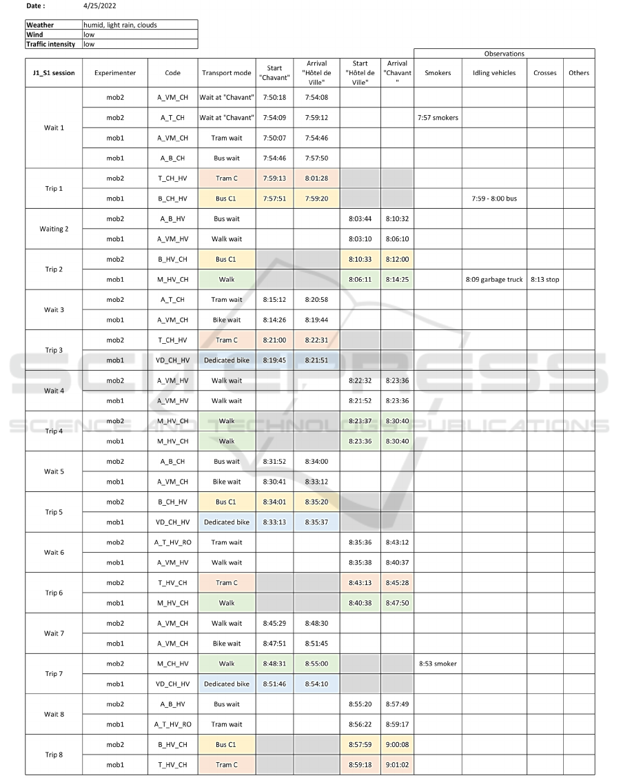
APPENDIX

Example of a measurement session

A Low-Cost Sensors Study Measuring Exposure to Particulate Matter in Mobility Situations