Logic + Reinforcement Learning + Deep Learning: A Survey

Andreas Bueff and Vaishak Belle

University of Edinburgh, U.K.

Keywords:

Logic-Based Reinforcement Learning.

Abstract:

Reinforcement learning has made signiﬁcant strides in recent years, including in the development of Atari

and Go-playing agents. It is now widely acknowledged that logical syntax adds considerable ﬂexibility in

both the modelling of domains as well as the interpretability of domains. In this survey paper, we cover the

fundamentals of how logic, reinforcement learning, and deep learning can be uniﬁed, with some ideas for

future work.

1 INTRODUCTION

Reinforcement learning (RL) has made signiﬁcant

strides in recent years, including in the development

of Atari and Go-playing agents (Denil et al., 2016;

Foerster et al., 2016; Mnih et al., 2013). It is now

widely acknowledged that logical syntax adds consid-

erable ﬂexibility in both the modelling of domains as

well as the interpretability of domains (Milch et al.,

2005; Hu et al., 2016; Narendra et al., 2018; Graves

et al., 2014). In this survey paper, we cover the fun-

damentals of how logic, reinforcement learning, and

deep learning can be uniﬁed, with some ideas for fu-

ture work. In some cases, we go into some depth into

the technical details because the modules depend on

such details.

We begin with a brief review of inductive logic

programming (ILP), the main paradigm we focus on

in this article (Raedt et al., 2016). Although there

are other approaches, such as (Sanner and Kersting,

2010), which uses Partially-observable Markov deci-

sion processes (POMDPs) as a powerful model for

sequential decision-making problems with partially-

observed states, and those that apply satisﬁability

(SAT) logical representations in Discrete Hopﬁeld

Neural Networks (DHNN) (Zamri et al., 2022; Guo

et al., 2022; Chen et al., 2023), we focus on ILP be-

cause it allows the learning of rules, a powerful facet

for understanding the policies learned by agents, and

could play an important role in explainable AI (Bhatt

et al., 2020). After discussing the basics of RL, we

will delve into recent advances in extending ILP and

differential ILP, which allows for neural integration in

the learning of logical rules with RL.

2 LOGIC PROGRAMMING

Logic programming is a programming paradigm with

relational logic (Kowalski, 1974), composed of a tu-

ple (R, F) where R is a set of rules and F a set of facts.

This tuple encapsulates an if-then rule. Such rules are

known as clauses and a deﬁnite clause is a rule com-

posed of a head atom α and a body α

, ··· , α

, for-

mally α ← α

, ··· , α

with rules read from right to

left. In order for α to be true, all atoms to the right

must also be true. An atom α is a tuple p(t

, ··· , t

)

where p is a predicate with an arity of n in conjunc-

tive normal form (CNF). The body of the predicate is

deﬁned by the terms t

, ··· , t

which can be variables

or constants. To ground an atom means to have terms

deﬁned by constants (Evans and Grefenstette, 2017).

2.1 ILP

Inductive logic programming (ILP) is a method of

symbolic computing which can automatically con-

struct logic programs provided a background knowl-

edge base (KB) (Muggleton and de Raedt, 1994). An

ILP problem is represented as a tuple (B, P , N ) of

ground atoms, with B deﬁning the background as-

sumptions, P is a set of positive instances which help

in deﬁning the target predicate to be learned, and N

deﬁnes the set of negative instances of the target pred-

icate. The aim of ILP is to eventually construct a

logic program that explains all provided positive sets

and rejects the negative ones. Given an ILP problem

(B, P , N ), the aim is to identify a set of hypothe-

ses (clauses) H such that (Muggleton and de Raedt,

1994):

• B ∧H |= γ for all γ ∈ P

• B ∧H 6|= γ for all γ ∈ N

Bueff, A. and Belle, V.

Logic + Reinforcement Learning + Deep Learning: A Survey.

DOI: 10.5220/0011746300003393

In Proceedings of the 15th International Conference on Agents and Artiﬁcial Intelligence (ICAART 2023) - Volume 3, pages 713-722

ISBN: 978-989-758-623-1; ISSN: 2184-433X

 2023 by SCITEPRESS – Science and Technology Publications, Lda. Under CC license (CC BY-NC-ND 4.0)

713

Where |= denotes logical entailment. Thus

stating, that the conjunction of the background

knowledge and hypothesis should entail all

positive instances and the same should not

entail any negative instances. We assume

for example a KB with provided constants

{bob, carol, volvo, jacket, pants, skirt, ···}, where

the task is to learn the predicate Passenger(X).

Then the ILP problem is deﬁned as:

• B = {Car( f ord), Clothing( jacket),

On( jacket, bob), Inside(carol, volvo), ···}

• P = {Passenger(bob), Passenger(carol), ···}

• N = {Passenger(volvo),Passenger( jacket),···}

The outcome of the induction performed is a hypoth-

esis of the form:

Passenger(X) ← Inside(X,Y

) ∧Car(Y

) ∧On(Y

, X)

∧Clothing(Y

)

The learned ﬁrst-order logic rule from the KB states

“if an object is inside the car with clothing on it, then

it is a passenger”.

The ILP problem may also contain a language

frame L and program template Π (Evans and Grefen-

stette, 2017). The language frame is a tuple which

contains information on the target predicate, the set

of extensional predicates, the arity of each predicate,

and a set of constants, while the program template de-

scribes the range of programs that can be generated.

2.2 dILP

To make ILP more robust to noise in data, Evans et al.

expanded the framework by making it differentiable

(Evans and Grefenstette, 2017). Doing so provides a

loss function which can be minimised with stochas-

tic gradient descent. Differential inductive logic pro-

gramming (dILP) utilises a continuous interpretation

of semantics where atoms are mapped to values [0,1].

dILP requires a valuation vector [0, 1]

with n atoms

which map each ground atom γ ∈ G to a real unit in-

terval. Also deﬁned is an atom label Λ which pairs a

true binary identiﬁer λ to atoms in P (λ = 1) and false

binary to atoms in N (λ = 0).

Provided an ILP problem (L, B, P , N ), a pro-

gram template and class weights W . The differential

model we are trying to solve for an atom α is

p(λ|α,W, Π, L, B) where λ acts as a classiﬁcation

problem for α. Thus, this sets our goal as minimising

the expected negative log-likelihoods for pairs (α, λ).

loss = −E

(α,λ)∼Λ

[λlog p(λ|α,W, Π, L, B) +

(1 −λ) log p(1 − p(λ|α,W, Π, L, B))]

By forward chaining T steps, we can calculate the

consequences of applying the rules, so-called “Con-

clusion Valuation”. The probability of λ given α is

computed using the auxiliary functions f

exract

, f

in f er

covert

, and f

generate

. We refer to the literature (Evans

and Grefenstette, 2017) for further details on the cal-

culations of the remaining auxiliary functions.

2.3 dNL

Payani et al. proposed an extension to ILP called dif-

ferentiable neural logic (dNL) networks which utilise

differentiable neural logic layers to learn Boolean

functions (Payani and Fekri, 2019). The concept is

to deﬁne Boolean functions that can be combined in a

cascading architecture akin to neural networks. Giv-

ing deep learning an explicit symbolic representation

that is interpretable, and redeﬁnes ILP as an optimisa-

tion problem. The dNL architecture uses membership

weights and conjunctive and disjunctive layers with

forward chaining to remove the need for the rule tem-

plate to solve ILP problems.

Payani et al. mapped Boolean values (true =

1, f alse = 0) to real value ranges [0, 1], and deﬁned

fuzzy unary and dual Boolean functions of variables

x and y as follows:

• x = 1 −x

• x ∧y = xy

• x ∨y = 1 −(1 −x)(1 −y)

Given an input vector x

into the logical neuron, the

implementation of the conjunction function requires

ﬁrst selection of a subset of x

and applying mul-

tiplication(conjunction) of selected elements. Train-

able Boolean membership weights m

are also associ-

ated with each input element x

from vector x

. The

conjunction function in Equation 1 is deﬁned by the

Boolean function deﬁned in Equation 2 which is able

to include each element in the conjunction function.

con j

) =

∏

i=1

, m

) (1)

, m

) = x

= 1 −m

(1 −x

) (2)

By combining different Boolean functions, a

multi-layered structure can be created. For example,

cascading a conjunction function with a disjunction

function( see Equation 3) creates a layer in disjunc-

tion normal form (DNF), so-called dNL-DNF.

dis j

) = 1 −

∏

i=1

(1 −F

, m

)) (3)

, m

) = x

(4)

ICAART 2023 - 15th International Conference on Agents and Artiﬁcial Intelligence

714

A dNL conjunction function F

is associated with

the i

rule of intensional predicate p in a logic pro-

gram and the membership weights m

act as Boolean

ﬂags to each atom. As membership weights can be

optimised, we ﬁnd that dNL is similar to dILP. How-

ever, dILP maps Boolean ﬂags to permutations of

two atom sets and only uses the weights to infer the

Boolean ﬂags in selecting a single winning clause.

We refer the reader to (Payani and Fekri, 2019) for

a further description of the forward chaining for eval-

uation.

3 REINFORCEMENT LEARNING

Reinforcement learning (RL) seeks to solve the prob-

lem where an agent is tasked with learning an opti-

mal action sequence to maximise the expected future

reward (Sutton et al., 1998; Rodriguez et al., 2019).

The environment E that an agent operates on is of-

ten modelled as a Markov Decision Process (MDP).

An MDP is deﬁned as a tuple M = hS , A, R , T , Ei

where S is set of states, A is a set of actions that can

be taken, R : S ×A ×S is the reward function which

takes as input the current state s

, current action a

and provides reward from the transition to state s

t+1

R (s

, a

, s

t+1

). T : S ×A ×S is the transition prob-

ability function which represents the probability of

transitioning to state s

t+1

from state s

given action

was taken p(s

t+1

, a

). E ⊂S are the set of termi-

nal states (Sutton et al., 1998; Leike et al., 2018). A

discount factor γ ∈ [0, 1] states how important it is to

receive a reward in the current state versus the future

state where R

∑

∞

k=0

t+k

is the total accumulated

return from the time step. The value function V

(τ) =

] of a policy is the measure of the expected sum

of discounted rewards r

. The objective is to ﬁnd the

optimal policy π(s) : S → A to maximise the reward

over time deﬁned by π

∗

= argmax

∑

∞

t=0

= s]

(Sutton et al., 1998; Rodriguez et al., 2019; Leike

et al., 2018; Roderick et al., 2017; Icarte et al., 2018;

Mnih et al., 2016). This is done by mapping a his-

tory of observations τ

= (a

, s

, a

, s

, ··· , a

t−1

, s

) to

the next action a

. In practice, at each time step t, the

agent is in a particular state s

∈S , select an action a

and according to π(·|s

), executes a

Value Based Methods: depend on V

to ﬁnd the

best action to take for each state. This method beneﬁts

from ﬁnite states. The Q-function value Q

(s, a) =

E[R

= s, a] under a policy π is the expected return

for selecting action a in state s and following policy π.

The Q-function updates using the Bellman equation,

where the Bellman equation is a fundamental relation-

ship between the value of a state action pair (s,a) and

the value of subsequent state-action pair (s

, a

) (Sut-

ton and Barto, 2012).

(s, a) = r + γE

, a

)], a

v π(s

) (5)

∗

(s, a) = arg max

(s, a) (6)

For deep learning and the Q-function, we parame-

terise the Q function Q(s,a; θ) where the action value

function is represented by a neural network.

Policy Based Methods: seek to directly learn a

policy π

(s), parameterised by θ as opposed to a value

function as in Q-learning. This is useful when the ac-

tion space is continuous or stochastic. Gradient as-

cent on E[R

] is done to update the parameters θ for a

parameterised policy π(a|s;θ). REINFORCE is a pol-

icy based algorithm that updates policy parameters θ

in the direction δ

logπ(a

;θ)R

which is an unbi-

ased estimate of δ

E[R

]. By subtracting the learned

function of the state, the baseline b

), it is possible

to reduce the variance of the estimate. The resulting

gradient is δ

logπ(a

;θ)(R

−b

)) (Sutton et al.,

1998; Mnih et al., 2016).

A mixed approach which takes advantage of both

value and policy-based methods is Actor-Critic where

a learned estimate of the value function is commonly

used as the baseline b

) = V

) leading to a lower

variance estimate of the policy gradient. The quan-

tity R

−b

used in the policy gradient can be seen as

an estimate of the advantage of action a

in state s

or A(a

, s

) = Q(a

, s

) −V (s

) because R

is an esti-

mate of Q

, st) and b

is an estimate of V

). The

critic estimates the value function which can be either

(a, s) or V

). The actor updates the policy dis-

tribution in the direction suggested by the critic via

policy gradients (Sutton et al., 1998).

A model is the internal representation of the en-

vironment for an agent, and this is often represented

with the transition function T and the reward function

R in an MDP. For RL, the approach with regard to

models is either model-based or model-free. Model-

based methods tasks an RL agent where the model is

input and an agent learns a policy through interact-

ing with the model, so-called planning. The opposite

of planning is seen with the trial and error approach

of model-free which relies on learning state and ac-

tion values to achieve a goal, solely through interact-

ing with the environment (Sutton et al., 1998). While

model-free methods lack sample efﬁciency from us-

ing a model, they tend to be easier to implement and

tune.

With planning, the agent’s observation of the en-

vironment results in the computation of the optimal

policy with respect to the model. The policy in this

framework describes a series of actions over a ﬁxed

Logic + Reinforcement Learning + Deep Learning: A Survey

715

time window to achieve a goal. The agent executes

the ﬁrst action of a plan then discards the rest and

sees to it that each interaction with the environment

generates a new plan.

Model-free methods include policy optimisation

methods, where the parameters for a policy are

learned via gradient ascent on the performance ob-

jective J(π

). Here the learning is done on-policy so

each update uses information learned while acting in

accordance with the most recent version of the policy.

Q-learning is the other model-free method which is

off-policy and learns the optimal action-value func-

tion Q

∗

(s, a) so each update uses information col-

lected at any point during training.

3.1 Relational RL

Relational Reinforcement learning (RRL) seeks to

combine ILP or relational learning with the general

RL framework. RRL has found applications in plan-

ning tasks (model-based) such as the simple block

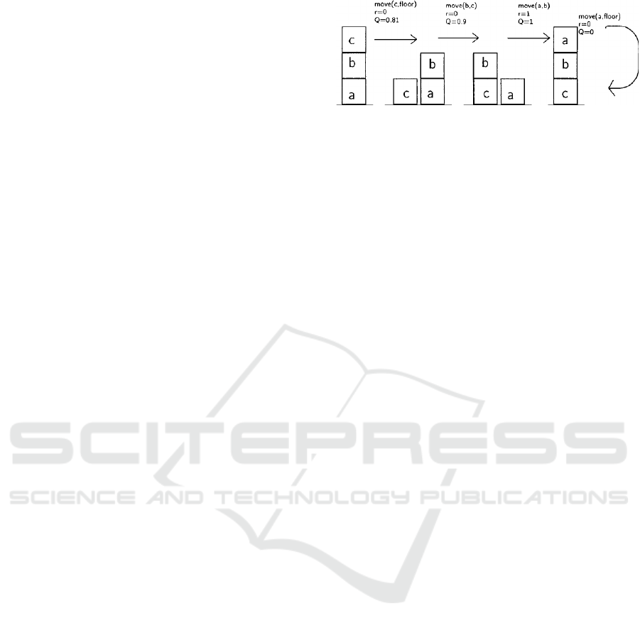
world task seen in Figure 1. RRL like classic RL is

tasked with learning a policy that provides agents with

the optimum actions to take in a given state. As RRL

integrates ILP, a state is represented relationally as a

set of ground facts. As a symbolic approach, RRL

learns ﬁrst-order logic (FOL) rules as a policy for a

given task (Driessens, 2010).

As RRL initially was developed for planning

(Driessens, 2010) the block worlds problem was

used as a basis for testing. The objective in

planning problems is to start from a state s and

ﬁnd a sequence of actions a

, ··· , a

with a

∈

A such that goal((··· , (s, a

))··· , a

n−1

) = true and

pre((···(s, a

)··· , a

i−1

), a

) = true. In the case of

block worlds, say we have 3 blocks called a, b, c on

the f loor, then states can be described by blocks ei-

ther being on each other or the ﬂoor, and actions

are represented by move(x, y) where x 6= y and x ∈

{a, b, c}, y ∈ {a, b, c, f loor}. An example state is

given:

= {clear(a), on(a, b), on(b, c), on(c, f loor)}

The initial work into RRL (Driessens, 2010) used

a modiﬁed Q-learning algorithm with a standard

relational learning algorithm (TILDA). Background

knowledge (BK) provides general predicates that can

be used for induction, where predicates are valid for

all training examples. As BK is prior knowledge de-

ﬁned in an expert-deﬁned predicate language, RRL

allows experts to input inductive biases to restrict the

search space. This not only provides policies that are

crafted for the expert’s interpretation but also speeds

up the learning process (Payani and Fekri, 2020).

Figure 1: Relational reinforcement learning in the box

world environment (Driessens, 2010).

RRL provides several beneﬁts over classical RL:

(1) The learned policy is human interpretable and can

be analysed by an expert. (2) The learned RRL policy

is also better able to generalise than policies learned

under classical RL. (3) As the language framework

for deﬁning states and actions is reliant on the expert,

inductive bias can be injected into learning which en-

tails that the expert can control agent behaviour to a

degree. (4) RRL allows for prior background knowl-

edge to act as heuristics in learning (Driessens, 2010;

Payani and Fekri, 2020).

Formally, the task formulation of RRL is given as:

1. States are described relationally using predicates.

2. Actions are described with relational language

such as that in the box world.

When combined with Q-learning, the standard

RRL algorithm uses the stochastic selection of ac-

tions and a relational regression tree. Similarly, the

Q-values are instantiated to zero.

Recent works in RRL have sought to learn end-

to-end in order to avoid the restrictions of regression

trees. In work done by Jiang et al. RRL is extended to

learn FOL policies with policy gradients (Jiang and

Luo, 2019). The authors apply dILP to sequential

decision-making tasks such as the block world task

and cliff walking task.

Taking dILP’s valuation vector e, the authors ex-

pand on its architecture to create so-called Differen-

tial recurrent logic machines (DRLM) which perform

iterative deduction on the valuation vector by taking

the probabilistic sum of possible grounded atoms a

and b, denoted as ⊕ and deﬁned as a⊕b = a+b−a

b, where  is the component-wise product. DRLM

treats the valuation produced by the last step deduc-

tion only as input, so the last step of the deduction is

just a function of the initial valuation vector e

and

the sum of the deduced valuation. DRLM also ex-

tends the expressiveness of dILP policies by assigning

weights to individual clauses whereas dILP is limited

to combinations of clauses (Jiang and Luo, 2019).

) =

(

( f

t−1

)), if t ≤ 0

, if t = 0

(7)

ICAART 2023 - 15th International Conference on Agents and Artiﬁcial Intelligence

716

The deduction of facts e

using weights w for in-

dividual clauses is done iteratively. Each iteration de-

composes the valuation vector with a single-step de-

duction function g

as seen in Equation 7 where t is

the deduction step. The single-step deduction func-

tion g

takes in the clause weights and valuation vec-

tor on the clause, as seen in Equation 8.

(e) = (

⊕

∑

n, j

(e)) +e

(8)

The function F

n, j

performs one step deduction on the

valuation vector e with the j

deﬁnition of the n

clause.

The authors rely on encoders and decoders to

translate ﬁrst-order atoms to policy valuation and ac-

tionable policy for the agent. The state encoder p

S →2

maps game world states to sets of atoms, and

the decoder p

: [0, 1]

|D|

→ [0, 1]

|A|

maps atoms back

to actions. The authors trained their agent using the

REINFORCE algorithm and the design of the encoder

and decoder architecture was done with neural net-

works. In order to ensure the system is differentiable,

they represent the probability of actions based on the

valuations e.

(a|e) =

(

l(e,a)

, if σ ≥ 1

l(e,a)

1−σ

|A|

, if σ < 1

(9)

Here, we have the valuation vector e determining

the value of a given action. The ﬁrst case is the pro-

portional value of an action where the total sum of the

valuations is over 1, and if the sum of values is less

than one total valuation is evenly distributed to all ac-

tions. The function l : [0, 1]

|D|

×A → [0, 1] maps the

valuation vector to the valuation of that action atom

and σ is the sum of all action valuations

∑

l(e, a).

As a model-based approach, Neural Logic Rein-

forcement Learning (NLRL) is limited to learning in

a discrete space. Zambaldi et al. sought to extend

RRL to a model-free and continuous-based setting by

taking advantage of Deep RL and relational learning

(Zambaldi et al., 2019). The authors incorporate re-

lational inductive bias for entity and relation-focused

representations by applying an iterative relational rea-

soning mechanism. In an environment, entities cor-

respond to local regions of an image and the agent

learns the values of certain entities and compares their

interactions with other entities. Visual data is handled

by a convolutional neural network (CNN) front-end

and the agent itself learns with the off-policy A2C al-

gorithm.

For the actor, the policy consists of logits over a

set of possible actions, and the critic generates a base-

line value which is used to calculate the temporal-

difference error to optimise π. As mentioned, input

for the agent is done via a CNN which takes an image

from a game environment and transforms it into an

embedded state representation. Entity vectors E are

computed by transforming an m ×n × f feature ma-

trix to an N × f matrix where (N = m ·n) and where

f represents the number of feature maps. This allows

each row e

in E to correspond to a feature vector s

x,y

for any point location x, y in the state image.

The authors tested their framework on the block-

worlds problem and on the popular real-time strategy

(RTS) game Starcraft 2. The lack of a formal ILP

module prevents the policies from being represented

in a FOL language, losing some human interpretabil-

ity. The relational model proposed by the authors is

deﬁned as a stack of multiple relational blocks, and

these blocks perform one-step relational updating us-

ing a shared recurrent neural network (RNN) on un-

shared parameters to derive higher-order entity rela-

tions.

Relational reasoning on the entity interactions is

performed by taking the entity interactions p

i, j

and

updating each entity based on interactions in the gam-

ing environment. The self-attention network, so-

called multi-head dot-product attention (MHDPA),

projects the entities E into matrices query (Q), key

(K), and value (V ) to compute the similarities. The

dot product is taken for a query q

and all keys k

j=1:N

which are then normalised via a softmax function into

attention weights w

The pairwise interactions are computed using the

attention weights and value matrix p

i, j

= w

i, j

. The

equation 10 deﬁnes the transformation performed to

derive the accumulated interactions with d deﬁning

the number of dimensions of the Q and K matrices

(N ×d).

A = so f tmax



√



V (10)

Updates to the entities E

is done via a multi-layer

perception (MLP) g

which takes as input the accu-

mulated interactions e

= g

h=1:H

Another approach for end-to-end learning with

model-based agents is the work by Dong et al. In their

work they develop so-called, Neural Logic Machines

(NLM), for a variety of relational reasoning tasks in-

cluding the RRL setting of the block worlds problem

(Dong et al., 2019). Like NLRL, NLM is able to

learn lifted rules from a policy which are generalis-

able and handle high-order relational data, for exam-

ple, the transitional rule r(a, c) ← ∃b r(a, b) ∧r(b, c)

where reasoning is performed on objects (a, b, c). An-

other common issue addressed in this work is that of

ILP’s issue with scaling. In (Yang and Song, 2019),

Logic + Reinforcement Learning + Deep Learning: A Survey

717

MLPs for NLRL act as decoders/encoders while in

the following work, MLPs are integrated into the rule

evaluation and generation process.

The logical framework of ILP is refactored as so-

called logic predicate tensors. The NLM architec-

ture allows for neural-symbolic realisations of Horn

clauses in FOL. A Horn clause is a clause with at most

one positive literal such that a rule ˆp ← p

(x) ∧p

(x)

implies ∀ ˆp ← p

(x) ∧ p

(x). Using MLPs, an NLM

is able to learn logical operations such as AND and

OR. NLMs take as input a KB comparing base pred-

icates and variable objects. NLMs apply FOL rules

to draw conclusions using tensors to represent logic

predicates. Predicates are grounded with permuta-

tions of possible variable input and evaluated as being

true or false. The grounded predicates are represented

by logic tensors and implemented by neural operators

for a sequential logic deduction. The ﬁnal output is a

set of generalisable rules which contain the probabil-

ity of variables and their relations.

The authors combine a probabilistic view on a log-

ical predicate with their so-called U-grounding tensor

provided a set of variables U = {u

, u

, ··· , u

and predicates p(x

, x

, ··· , x

)-arity r, which can be

grounded as a tensor of size [m

ˆr

] where m

ˆr

is de-

ﬁned as [m, m −1, m −2, ··· , m −r + 1]. The prop-

erties of a variable are deﬁned here as unary predi-

cates “moveable(x)”, relations of predicates are de-

ﬁned as a binary predicate “on(x, y)”, and global prop-

erties are nullary predicates “allmatched()”. The

grounding of each entity p

, u

, ··· , u

) repre-

sents whether p is true provided a given instantiation.

The authors extend this representation of a logic

predicate p

by stacking them, they deﬁne C

(r)

to be

the number of predicates of arity r. This creates a

tensor of size [m

ˆr

(r)

]. NLM applies a probabilis-

tic interpretation by taking each ground predicate and

deriving a likelihood ∈ [0, 1] for being true.

The modules of the architecture are reliant on

select meta-rules. (1) Boolean logic rules for op-

erations AND, OR, NOT and (2) quantiﬁcations

which link predicates of different arities via logic

quantiﬁers (∀, ∃). The neural Boolean logic rule

is predicate logic in the form ˆp(x

, x

, ··· , x

) ←

expression(x

, x

, ··· , x

) and can be deﬁned as an ex-

ample moveable(x) ← ¬isground(x) ∧clear(x). In

the context of NLM, provided a set of predicates

P = {p

, p

, ··· , p

} with all the same arity, they can

be stacked as a tensor of shape [m

ˆr

, |P|] with arbitrary

permutations of potential groundings. An MLP takes

as input all the permutations of p

to create r! tensors

with shape [m

ˆr

, r! ×|P|] as well as trainable parame-

ters θ. A sigmoid is applied to the MLP to derive the

likelihood of a speciﬁc predicate.

The neural quantiﬁers are deﬁned by two rules, (1)

Expansion which constructs a new predicate q from p

by introducing a new variable x

r+1

, where x

r+1

is not

a previous variable in the body of the predicate:

∀x

r+1

q(x

, x

, ··· , x

, x

r+1

) ← p(x

, x

, ··· , x

) (11)

The Expand() method, given a set of C r-arity

predicates with a shape [m

,C], expands the logic

predicate tensor by the addition of a distinct variable

r+1

. The additional dimension to the tensor creates a

shape [m

r+1

,C]. The second rule is reduction, where

using either the ∀, ∃ quantiﬁer, reduces the arity of a

body request by marginalising over a given variable.

q(x

, x

, ··· , x

) ← ∀x

r+1

p(x

, x

, ··· , x

, x

r+1

) (12)

The implementation Reduce() is just the reverse

architecture of Expand() where given a [m

r+1

,C]

shaped tensor with a set of C

(r+1)

-arity predicates re-

duces the tensor along the x

r+1

dimension by taking

the max and min and stacking the resulting tensors for

a dimension of [m

ˆr

, 2C].

The authors combine these meta-rules to create

the formal NLM, comprising D layers with B + 1

computations per layer. NLM computes one split

into two distinct computational phases. Provided an

input layer O

i−1

to produce the output layer O

(0)

, O

(1)

, ··· , O

(B)

}. The inter-group computation

relies on Equation 11 and 12 which takes in tensors

from say layer i and connects the previous layer i −1

into vertically neighbouring groups of arity r, r + 1,

etc. Aligning of the dimensions is done by Reduce()

or Expand() to form the tensor I

(r)

= Concat(Expand(O

(r−1)

i−1

), O

(r)

i−1

, Reduce(O

r+1

i−1

))

(13)

This addresses the issue of the aligning predicates of

the proximal arities and different orders.

Intra-group computation takes the tensor from the

inter-group computation I

(r)

and permutes the predi-

cate inputs to produce the output tensor O

(r). The

ﬁnal output shape of the tensor is [m

ˆr

(r)

= σ(MLP(Permute(I

(r)

;θ

(r))). (14)

Taking the concepts of dNL (Section 2.3), Payani

et al. combine their dNL framework with RL (Payani

and Fekri, 2020). Like NLRL, the author test on the

block world gaming environment and take advantage

of the declarative bias with provided BK. The authors

seek to expand RRL to handle complex scene inter-

pretations similarly to standard deep RL. Payani et

al. take their dNL-ILP differentiable deductive engine

ICAART 2023 - 15th International Conference on Agents and Artiﬁcial Intelligence

718

to give RRL an end-to-end learning framework, so-

called dNL-RRL. This allows for a deep RL approach

with ILP. The authors focus on-policy gradients in or-

der to improve interpretability and also regression in

the form of expert constraints.

RRL has been limited in the past by non-

differentiable ILP (Muggleton and De Raedt, 1994),

so we have seen an overreliance on explicit relational

representations of states and actions in the BK. Hav-

ing differentiable ILP with the dNL-ILP engine al-

lows an RRL agent to learn from raw pixels to extract

low-level relational representations from CNNs. The

authors made signiﬁcant changes to the original RRL

algorithm with regard to the state representation, lan-

guage bias, and action representation.

In the ﬁrst case, state representations, the objec-

tive is to take advantage of dNL-ILP for policy learn-

ing by extracting explicit state representations via

deep learning methods. The authors propose ﬁrst pro-

cessing raw images with CNNs and having the last

layer act as a feature vector which can contain info

such as pixel point position (x, y). Then feed the fea-

ture map into a relational unit to extract non-local fea-

tures (this approach is similar to that seen with (Zam-

baldi et al., 2019)), however, they do not rely on graph

networks instead seeking explicit predicates for ILP).

Three strategies are implemented for learning the

desired relational states from raw input. Where lower-

level state representations are ﬁrst learned by CNNs

trained on the raw input, followed by the abstraction

to higher-level representations. For example, a high-

level predicate on(X,Y ) can be deﬁned by position

predicates posH(X ,Y) and posV (X,Y) for X repre-

senting the block and Y the coordinates with posH

referring to the horizontal axis and posV the vertical

axis. The second strategy is state constraints, which

rely on the regularisation of the loss function and

connects to logic constraints for relational reasoning.

This requires the modeller to deﬁne what heuristics to

constrain. For example, posV ( f loor) should always

be zero. The third strategy is a semi-supervised set-

ting, where the modeller provides input which deﬁnes

certain states with labels to aid the agent in learning.

This information is added to the loss function as well.

The action representation is handled by having the

action probability distribution mapped to the ground-

ing of true predicates, for example, move(X,Y ) infer-

ring possible permutations of move(X,Y ) that are true

in a given state. In the case of multiple true predicates

of move(X,Y ), the probability distribution can be esti-

mated by applying a softmax function to the valuation

vector on the learned predicate move.

Outside of RRL, other avenues seeking to com-

bine RL with symbolic learning or explanations have

also been explored. Similar to the abstraction ap-

proach of Payani et al., Verma et al. also pur-

sued a similar approach in their contribution (Verma

et al., 2018), where the authors present Programmat-

ically Interpretable Reinforcement Learning (PIRL)

and Neurally Directed Program Search (NDPS). PIRL

is able to present policies in a human-readable lan-

guage, not unlike the dNL-ILP policies. The parame-

ters of PIRL include a high-level programming lan-

guage to deﬁne policies. These parameters infer a

policy(sketch) which deﬁnes the declarative language

for an RL problem in a high-level format. The ideal

policy(sketch) uses a language to maximise long-

term reward. The primary beneﬁts of PIRL’s lan-

guage are ﬁrst the interpretable output, followed by

encoding the modeller’s bias, effective pruning of un-

desired policies, and then a symbolic program veriﬁ-

cation method analogous to ILP. The authors also pro-

pose NDPS which uses Deep RL to compute a high-

performing yet non-interpretable policy in an RL en-

vironment. Inspired by imitation learning (Ho and

Ermon, 2016), the authors take the high-performing

policy and treat it as an oracle for searching out an in-

terpretable policy deﬁned by PIRL. An interpretable

policy is iteratively selected to minimise the output

difference between the high-performance policy and

itself.

An older approach by Garnel et al. establishes the

neural back-end and symbolic front-end framework

seen so far (Garnelo et al., 2016). The authors com-

bine deep learning with classical symbolic AI, inte-

grating symbolic elements such as constants, func-

tions, and predicates. Garnele et al. note the limi-

tation of declarative bias in instantiating symbolic se-

mantics for an RL agent to interpret. The back-end

works similarly to an auto-encoder to compress raw

perceptional data to be fed as input to the symbolic

front-end which maps the inputs to actions. The au-

thors also propose a set of principles, which are rel-

evant to all research with regard to symbolic RL. (1)

Conceptual abstraction which determines whether a

new situation is similar to past experiences and can

a connection be drawn. (2) Compositional struc-

ture which is a representational medium that has a

set of elements that can be recompiled in an open-

ended manner such as probabilistic FOL. (3) Com-

mon sense priors are the minimal assumptions and

expectations that can be built into the learning pro-

cedure and (4) Causal reasoning which attempts to

discover the causal structure of the domain and ex-

press them through the common sense ontology pro-

vided. This work was further extended by Garcez

et al. (d’Avila Garcez et al., 2018) by providing

heuristics to the common sense principle, so-called

Logic + Reinforcement Learning + Deep Learning: A Survey

719

principle one which only updates agent and object

interaction states based on Q values only when the

rewards are non-zero and principle two which takes

into account the relational position of an object to an

agent as a factor for an action selection.

In (Martires et al., 2020), real-world perception in

an RL setting was researched where a semantic world

modelling approach via detecting, segmentation, and

processing perceived objects from visual input and

then applying an anchoring system to maintain con-

sistent representations (anchor) of perceived objects.

The pipeline ends with an inference system to self-

check the anchoring system and for logically tracking

objects in a dynamic setting. Predicate logic is used

as the language for relational representation.

In (Li et al., 2019), the graph network approach

to real-world robotics tasks is also interesting to note.

Graph networks provide an alternative to ILP since

graph structures are suitable for an object-oriented en-

vironment and can model relational relationships be-

tween objects. Li et al. have an agent train with

an attention-based graph neural network (GNN) to

handle curriculum learning with multi-object environ-

ments and have the number of objects increase as the

agent learns.

Other works have provided a testing bed for RRL

research such as the works by Silver et al. (Silver

and Chitnis, 2020). The authors bridge the research

environment Open AI Gym (Brockman et al., 2016)

with planning domains in Planning Domain Deﬁni-

tion Language (PDDL) which allows for testing of RL

interpretability.

Zhang et al. combine high-level symbolic rules

and deep Q-learning (DQN), treating rules deﬁned in

a knowledge background as intuitive heuristics such

as “slow down when you approach curve” (Zhang

et al., 2019). The authors proposed so-called, Rule-

interposing Learning (RIL), which has a deep learn-

ing component. An agent queries the KB for appro-

priate actions in addition to Q values and decides what

action is appropriate. The KB aids the DQN in prun-

ing the actions that are unsafe or unnecessary. The KB

acts as an independent module, as opposed to (Gar-

nelo et al., 2016), which relies on the end-to-end RL

architecture with neural back-end and symbolic front-

end.

Saebi et al. address the issue of knowledge graph

(KG) completion, and problems of inferring missing

relations in their work (Saebi et al., 2020). A real-

world KG can contain exponential numbers of entity

relations, overburdening an RL agent. The authors

propose a representation of the state space which in-

cludes entity-type information. They then use a prun-

ing algorithm to limit searches made by an agent in

the action space. Similarly (Li et al., 2019), the au-

thors use GNNs to encode neighbourhood informa-

tion.

Sreedharan et al. research into RRL explore so-

called, Expectation-aware planning, which includes a

‘human in the loop’ for agent learning. The authors

propose self-explaining plans which contain actions

that are responsible for explaining the plan in an inter-

pretable manner and seek to include agent behaviour

acting in accordance with human expectation (Sreed-

haran et al., 2019).

Pacheo et al. seek to combine GNNs and end-to-

end learning of deep learning in their seminal work

(Pacheco et al., 2018). The authors present DRail,

a declarative modelling language which consists of

rules sets with factor templates over variables. Rules

in the framework have an associated neural architec-

ture to learn a scoring function and feature deﬁnition.

A unique application, Lederman et al. rely on

graph networks and relational RL, primarily for solv-

ing quantiﬁed Boolean logics and returning proofs.

Here they utilise a GNN to predict the quality of

each variable as a decision variable to select an action

and use end-to-end learning to improve reasoning on

given sets of formulas (Lederman et al., 2018).

4 CONCLUSIONS

In this survey paper, we studied the various dimen-

sions and some technical foundations for logic + rein-

forcement learning + deep learning. There is a grow-

ing body of work on logic and deep learning (Garcez

et al., 2015), and this survey pushes the area further

by looking at dynamic domains. In an extended re-

port, we also discuss advances in inverse RL (Ng and

Russell, 2000) and its integration with ILP.

ACKNOWLEDGEMENTS

This research was partly supported by a Royal Soci-

ety University Research Fellowship, UK, and partly

supported by a grant from the UKRI Strategic Priori-

ties Fund, UK to the UKRI Research Node on Trust-

worthy Autonomous Systems Governance and Regu-

lation (EP/V026607/1, 2020–2024).

REFERENCES

Bhatt, U., Xiang, A., Sharma, S., Weller, A., Taly, A., Jia,

Y., Ghosh, J., Puri, R., Moura, J. M. F., and Eckersley,

ICAART 2023 - 15th International Conference on Agents and Artiﬁcial Intelligence

720

P. (2020). Explainable machine learning in deploy-

ment. Proceedings of the 2020 Conference on Fair-

ness, Accountability, and Transparency.

Brockman, G., Cheung, V., Pettersson, L., Schneider, J.,

Schulman, J., Tang, J., and Zaremba, W. (2016). Ope-

nai gym. CoRR, abs/1606.01540.

Chen, J., Kasihmuddin, M. S. M., Gao, Y., Guo, Y., Asyraf

Mansor, M., Romli, N. A., Chen, W., and Zheng, C.

(2023). Pro2sat: Systematic probabilistic satisﬁability

logic in discrete hopﬁeld neural network. Advances in

Engineering Software, 175:103355.

d’Avila Garcez, A. S., Dutra, A. R. R., and Alonso, E.

(2018). Towards symbolic reinforcement learning

with common sense. CoRR, abs/1804.08597.

Denil, M., Agrawal, P., Kulkarni, T. D., Erez, T., Battaglia,

P., and de Freitas, N. (2016). Learning to perform

physics experiments via deep reinforcement learning.

Dong, H., Mao, J., Lin, T., Wang, C., Li, L., and

Zhou, D. (2019). Neural logic machines. CoRR,

abs/1904.11694.

Driessens, K. (2010). Relational Reinforcement Learning,

pages 857–862. Springer US, Boston, MA.

Evans, R. and Grefenstette, E. (2017). Learning explanatory

rules from noisy data. CoRR, abs/1711.04574.

Foerster, J. N., Assael, Y. M., de Freitas, N., and Whiteson,

S. (2016). Learning to communicate with deep multi-

agent reinforcement learning.

Garcez, A., Besold, T., De Raedt, L., F

oldi

ak, P., Hitzler, P.,

Icard, T., K

uhnberger, K.-U., Lamb, L., Miikkulainen,

R., and Silver, D. (2015). Neural-symbolic learning

and reasoning: Contributions and challenges.

Garnelo, M., Arulkumaran, K., and Shanahan, M.

(2016). Towards deep symbolic reinforcement learn-

ing. CoRR, abs/1609.05518.

Graves, A., Wayne, G., and Danihelka, I. (2014). Neural

turing machines.

Guo, Y., Kasihmuddin, M. S. M., Gao, Y., Mansor, M. A.,

Wahab, H. A., Zamri, N. E., and Chen, J. (2022).

Yran2sat: A novel ﬂexible random satisﬁability logi-

cal rule in discrete hopﬁeld neural network. Advances

in Engineering Software, 171:103169.

Ho, J. and Ermon, S. (2016). Generative adversarial imita-

tion learning. In Lee, D. D., Sugiyama, M., Luxburg,

U. V., Guyon, I., and Garnett, R., editors, Advances

in Neural Information Processing Systems 29, pages

4565–4573. Curran Associates, Inc.

Hu, Z., Ma, X., Liu, Z., Hovy, E. H., and Xing, E. P.

(2016). Harnessing deep neural networks with logic

rules. CoRR, abs/1603.06318.

Icarte, R. T., Klassen, T., Valenzano, R., and McIlraith,

S. (2018). Using reward machines for high-level

task speciﬁcation and decomposition in reinforcement

learning. In Dy, J. and Krause, A., editors, Pro-

ceedings of the 35th International Conference on Ma-

chine Learning, volume 80 of Proceedings of Ma-

chine Learning Research, pages 2107–2116, Stock-

holmsm

assan, Stockholm Sweden. PMLR.

Jiang, Z. and Luo, S. (2019). Neural logic reinforcement

learning.

Kowalski, R. A. (1974). Predicate logic as programming

language. In IFIP Congress, pages 569–574.

Lederman, G., Rabe, M. N., Lee, E. A., and Seshia, S. A.

(2018). Learning heuristics for quantiﬁed boolean for-

mulas through deep reinforcement learning.

Leike, J., Krueger, D., Everitt, T., Martic, M., Maini,

V., and Legg, S. (2018). Scalable agent alignment

via reward modeling: a research direction. CoRR,

abs/1811.07871.

Li, R., Jabri, A., Darrell, T., and Agrawal, P. (2019). To-

wards practical multi-object manipulation using rela-

tional reinforcement learning.

Martires, P. Z. D., Kumar, N., Persson, A., Loutﬁ, A., and

Raedt, L. D. (2020). Symbolic learning and reasoning

with noisy data for probabilistic anchoring.

Milch, B., Marthi, B., Russell, S. J., Sontag, D., Ong, D. L.,

and Kolobov, A. (2005). BLOG: Probabilistic models

with unknown objects. In Proc. IJCAI, pages 1352–

1359.

Mnih, V., Badia, A. P., Mirza, M., Graves, A., Lillicrap,

T. P., Harley, T., Silver, D., and Kavukcuoglu, K.

(2016). Asynchronous methods for deep reinforce-

ment learning.

Mnih, V., Kavukcuoglu, K., Silver, D., Graves, A.,

Antonoglou, I., Wierstra, D., and Riedmiller, M.

(2013). Playing atari with deep reinforcement learn-

ing.

Muggleton, S. and de Raedt, L. (1994). Inductive logic pro-

gramming: Theory and methods. The Journal of Logic

Programming, 19-20:629 – 679. Special Issue: Ten

Years of Logic Programming.

Muggleton, S. and De Raedt, L. (1994). Inductive logic

programming: Theory and methods. The Journal of

Logic Programming, 19:629–679.

Narendra, T., Sankaran, A., Vijaykeerthy, D., and Mani, S.

(2018). Explaining deep learning models using causal

inference. CoRR, abs/1811.04376.

Ng, A. Y. and Russell, S. J. (2000). Algorithms for inverse

reinforcement learning. In Proceedings of the Seven-

teenth International Conference on Machine Learn-

ing, ICML ’00, page 663–670, San Francisco, CA,

USA. Morgan Kaufmann Publishers Inc.

Pacheco, M. L., Dalal, I., and Goldwasser, D. (2018).

Leveraging representation and inference through deep

relational learning. NeurIPS Workshop on Relational

Representation Learning.

Payani, A. and Fekri, F. (2019). Inductive logic program-

ming via differentiable deep neural logic networks.

CoRR, abs/1906.03523.

Payani, A. and Fekri, F. (2020). Incorporating relational

background knowledge into reinforcement learning

via differentiable inductive logic programming.

Raedt, L. D., Kersting, K., Natarajan, S., and Poole, D.

(2016). Statistical relational artiﬁcial intelligence:

Logic, probability, and computation. Synthesis Lec-

tures on Artiﬁcial Intelligence and Machine Learning,

10(2):1–189.

Roderick, M., Grimm, C., and Tellex, S. (2017). Deep ab-

stract q-networks.

Logic + Reinforcement Learning + Deep Learning: A Survey

721

Rodriguez, I. D. J., Killian, T. W., Son, S., and Gombolay,

M. C. (2019). Interpretable reinforcement learning via

differentiable decision trees. CoRR, abs/1903.09338.

Saebi, M., Krieg, S., Zhang, C., Jiang, M., and Chawla, N.

(2020). Heterogeneous relational reasoning in knowl-

edge graphs with reinforcement learning.

Sanner, S. and Kersting, K. (2010). Symbolic dynamic

programming for ﬁrst-order pomdps. In Proc. AAAI,

pages 1140–1146.

Silver, T. and Chitnis, R. (2020). Pddlgym: Gym environ-

ments from pddl problems.

Sreedharan, S., Chakraborti, T., Muise, C., and Kambham-

pati, S. (2019). Planning with explanatory actions: A

joint approach to plan explicability and explanations

in human-aware planning. CoRR, abs/1903.07269.

Sutton, R. S. and Barto, A. G. (2012). Reinforcement Learn-

ing: An Introduction. The MIT Press.

Sutton, R. S., Barto, A. G., et al. (1998). Introduction to

reinforcement learning, volume 135. MIT press Cam-

bridge.

Verma, A., Murali, V., Singh, R., Kohli, P., and Chaudhuri,

S. (2018). Programmatically interpretable reinforce-

ment learning. CoRR, abs/1804.02477.

Yang, Y. and Song, L. (2019). Learn to explain efﬁciently

via neural logic inductive learning.

Zambaldi, V., Raposo, D., Santoro, A., Bapst, V., Li, Y.,

Babuschkin, I., Tuyls, K., Reichert, D., Lillicrap,

T., Lockhart, E., Shanahan, M., Langston, V., Pas-

canu, R., Botvinick, M., Vinyals, O., and Battaglia,

P. (2019). Deep reinforcement learning with rela-

tional inductive biases. In International Conference

on Learning Representations.

Zamri, N. E., Azhar, S. A., Sidik, S. S. M., Mansor, M. A.,

Kasihmuddin, M. S. M., Pakruddin, S. P. A., Pauzi,

N. A., and Nawi, S. N. M. (2022). Multi-discrete

genetic algorithm in hopﬁeld neural network with

weighted random k satisﬁability. Neural Computing

and Applications, 34(21):19283–19311.

Zhang, H., Gao, Z., Zhou, Y., Zhang, H., Wu, K., and Lin, F.

(2019). Faster and safer training by embedding high-

level knowledge into deep reinforcement learning.

ICAART 2023 - 15th International Conference on Agents and Artiﬁcial Intelligence

722