On the Future of Training Spiking Neural Networks

Katharina Bendig

1,2

, Ren

e Schuster

and Didier Stricker

1,2

Technische Universit

at Kaiserslautern, Germany

DFKI – German Research Center for Artiﬁcial Intelligence, Germany

{ﬁrstname.lastname}@dfki.de

Keywords:

Spiking Neural Networks, Surrogate Gradients, Supervised Training, ANN2SNN, Conversion.

Abstract:

Spiking Neural Networks have obtained a lot of attention in recent years due to their close depiction of brain

functionality as well as their energy efﬁciency. However, the training of Spiking Neural Networks in order

to reach state-of-the-art accuracy in complex tasks remains a challenge. This is caused by the inherent non-

linearity and sparsity of spikes. The most promising approaches either train Spiking Neural Networks directly

or convert existing artiﬁcial neural networks into a spike setting. In this work, we will express our view on

the future of Spiking Neural Networks and on which training method is the most promising for recent deep

architectures.

1 INTRODUCTION

Deep Learning (DL) is becoming more and more in-

ﬂuential both in our current daily lives as well as in

future research. There have been remarkable achieve-

ments in a variety of application areas, such as com-

puter vision (Krizhevsky et al., 2012), text process-

ing (Vaswani et al., 2017), autonomous driving (Chen

et al., 2017) and robotics (Andrychowicz et al., 2019).

Unfortunately, as the complexity of the applica-

tions grows, so does the size of the neural network

and the energy resources required during training and

inference. This leads not only to a higher carbon foot-

print but also to limited applicability on mobile de-

vices. It has been shown that costs grow roughly in

proportion to the demand for computing power, so we

are inevitably heading towards the point where DL is

no longer sustainable (Thompson et al., 2021). On

the other hand, the brain uses only a fraction of the

resources compared to a computer while performing

comparable or even more complex tasks and addition-

ally managing general functions of the body (Bala-

subramanian, 2021). This demonstrates that a great

deal of optimization and innovation is still required to

truly exploit the full potential of DL and neural archi-

tectures.

One possible approach is the usage of Spik-

ing Neural Networks (SNNs) (Gerstner and Kistler,

2002), which depict the biological functionality of

the brain more closely than traditional Artiﬁcal Neu-

ral Networks (ANNs). Spiking neurons communicate

by means of spikes, which can be represented solely

on the basis of ones and zeros. Therefore, theoreti-

cally no multiplications with synaptic weights like in

ANNs are necessary. The multiplication with zero re-

sults automatically in zero and a multiplication with

one in the weight itself, which only requires a single

memory read-out. Additionally, the inherent sparsity

of the spikes leads to a generally decreased amount of

computations in the network, since only the arrival of

spikes induces computations in the neuron. For these

reasons SNNs have the advantage of a lower energy

consumption during inference and training compared

to ANNs.

In theory, SNNs have been shown to possess

the same expressive power as ANNs (Maass and

Markram, 2004). However, practically there are still

many hindrances in the training of SNNs, so that in

the majority of cases they cannot reach the perfor-

mance capability of ANNs at the time being.

There are generally three ways to obtain a trained

SNN: Biological, conversion from a pre-trained

ANN, and direct training. The biological approach

typically leads to local optimization rules that are dif-

ﬁcult to extend to deep networks, (Nunes et al., 2022).

This can be avoided by utilizing an existing ANN and

converting it into a SNN, since this principle can be

applied to a variety of modern architectures (Rueck-

auer et al., 2017). However, restrictions are often im-

posed on the ANN and the conversion is in any case

an approximation, so that the resulting SNN usually

suffers from lower performance. There are also ob-

stacles associated with the direct training, since the

spiking functional is non-differentiable and thus the

466

Bendig, K., Schuster, R. and Stricker, D.

On the Future of Training Spiking Neural Networks.

DOI: 10.5220/0011745500003411

In Proceedings of the 12th International Conference on Pattern Recognition Applications and Methods (ICPRAM 2023), pages 466-473

ISBN: 978-989-758-626-2; ISSN: 2184-4313

 2023 by SCITEPRESS – Science and Technology Publications, Lda. Under CC license (CC BY-NC-ND 4.0)

successful gradient descent method is not directly ap-

plicable.

In this work, we will explore and compare

the advantages and disadvantages of these training

paradigms especially with regard to their use in fu-

ture real-world applications. This encompasses their

practicality in very deep neural networks as well as

their applicability for complex datasets. We are con-

vinced, that the future of SNNs lies in the direct train-

ing, due to its capability to train deep networks, its

greater variability concerning the encoding of input

data and its consideration of internal temporal rela-

tionships of SNNs.

2 RELATED WORK

2.1 Spiking Neural Networks

The general architecture of SNNs is analogous to the

structure of ANNs (Gerstner and Kistler, 2002). The

crucial difference lies in the functionality of the spik-

ing neurons, which implement biological processes in

a more detailed way. Spiking neurons have a mem-

brane potential U that grows in response to exter-

nal stimuli. If a certain threshold θ is exceeded, the

neuron ﬁres and thus transmits a spike via outgo-

ing synapses. However, since it is very improbable

that all spikes arrive at a neuron simultaneously, there

are additional temporal dynamics, which maintain the

membrane potential over a short period of time.

In experiments on nerves in frogs, these dynam-

ics were found to be comparable to those in a simple

resistor–capacitor circuit (Brunel and van Rossum,

2007). Inspired by this, the simple Leaky Integrate-

and-Fire (LIF) neuron model is nowadays often used

in DL implementations for SNNs. A discrete approx-

imation of the LIF model can be described in the fol-

lowing way (Wu et al., 2019):

U[t] = βU [t − 1]

| {z }

decay

+W X[t]

|{z}

input

−S

out

[t − 1]θ

| {z }

reset

, (1)

with β as the decay rate of the membrane potential,

W X[t] as the weighted input spikes and S

out

[t] ∈ {0, 1}

as the generated output spike. The exponential de-

cay of the membrane potential sustains the incoming

spike information for a short amount of time, while

also preserving the non-correlation between spikes

at too distant time steps. Especially when ANNs

are converted to SNNs, this decay is often disre-

garded which results in the Integrate-and-Fire (IF)

neuron model. Furthermore, in case the neuron ﬁres

the membrane potential gets reset by subtracting the

threshold. Outgoing spikes are generated, when the

membrane potential reaches the threshold:

out

[t] =

(

1, if U[t] > θ

0, otherwise.

(2)

However, this functionality is non-differentiable,

meaning that gradient descent is not applicable as in

conventional ANNs. For this reason, the training of

SNNs is still an ongoing research topic.

2.2 Data Handling

Since the calculations in SNNs are based on spikes,

input data such as intensity values in images must be

converted to a spike format. This is especially rel-

evant in the context of converting ANNs, since the

input encoding needs to abide certain restriction for

the converted SNN, which will be further explained

in Section 2.3. The two main approaches for encod-

ing ﬂoating points into spikes are temporal and rate

encoding.

The temporal encoding stores the information

within the timing of a single spike. For image data

this means that a high pixel intensity is encoded in an

earlier spike, while a low intensity pixel is mapped to

a later spike. In addition, a logarithmic mapping is ap-

plied to mimic processes in the retina (Dehaene, 2003;

Arrow et al., 2021). The main advantage of temporal

encoding is the low energy consumption, since the in-

put data is extremely sparse and thus requires minimal

computations and memory access. However at the

same time, the sparsity leads to an insufﬁcient amount

of training signals and can therefore result in dead

neurons. Furthermore, this encoding has a poor er-

ror tolerance, since similar classes can ﬁre at the same

time and no additional time step is taken into account

in order to compensate for this. Additionally, it re-

mains ambiguous which property should be described

by an earlier spike time. A high intensity pixel, for

example, may only describe background information

of an image and therefore initially provide little infor-

mation to the neural network. This becomes particu-

larly problematic with more complex input data and

has been insufﬁciently addressed, as most approaches

have only considered simple datasets such as MNIST

(Lecun et al., 1998).

Rate coding on the other hand stores the infor-

mation in the number of spikes N over a period of

time. Accordingly, in the most common rate coding

scheme, the average ﬁring rate v over the time win-

dow T can be deﬁned as follows:

v =

. (3)

On the Future of Training Spiking Neural Networks

467

This is typically modeled with a Poisson distribution

with a mean event rate proportional to the normalized

pixel intensity (Nunes et al., 2022). The occurrence of

rate coding in biological processes has been demon-

strated in several studies, (Adrian and Zotterman,

1926). It has the advantage of having a high error

tolerance, since numerous incoming spikes can excite

a neuron that previously failed to ﬁre. Furthermore,

in output neurons, subsequent output spikes can com-

pensate for errors and make it easier to distinguish

classes. In addition, a large number of spikes leads

to many training signals and accordingly a stronger

gradient signal. However, this results in a trade-off

in terms of higher energy consumption and training

time due to increased computational operations. Rate-

coding is especially important for conversion algo-

rithms. These methods create SNNs based on pre-

trained ANNs based on the assumption, that the in-

put data will be fed into the converted SNN in a rate-

coded manner.

Recently, several SNN methods have started to use

the direct encoding scheme (Zenke and Vogels, 2021),

in which the ﬂoating point values of the input data are

fed directly into the network. This means that the ﬁrst

neuron layer is used to convert these values into spikes

and thus adopt the functionality of body sensors. The

advantage of this approach is that the encoding does

not have to be explicitly predeﬁned in a manual man-

ner and is instead learned by the network.

Biologically, different types of information encod-

ing in spikes exist in the brain (Izhikevich, 2003). For

this reason, it is important to study different types of

encoding that ﬁnd a balance between trainability and

energy efﬁciency. In theory, there are an inﬁnite num-

ber of ways to represent information in the form of

spikes, there is no necessity to limit oneself only to

temporal or rate encoding.

The most natural type of input for SNNs is event-

based data, since it already consists of binary events

and is further sparse and asynchronous. For exam-

ple, Dynamic Vision Sensor (DVS) cameras can be

used to detect intensity changes above a threshold in

an asynchronous manner (Gallego et al., 2022). For

traditional ANNs, processing this type of data is chal-

lenging because they perform synchronous computa-

tions. Thus pre-training an ANN directly with event

data for later conversion into a SNN becomes chal-

lenging, (Deng et al., 2019).

2.3 Training of SNNs

Despite all the successes of DL, the brain still remains

the reference point due to its comprehensive precision

and efﬁciency. For this reason, there is still a great re-

search effort to understand the exact processes in the

brain. Nevertheless, it is still not possible to ﬁnd the

exact mechanism that allows the brain to learn com-

plex patterns and abstract thinking.

For traditional ANNs, the most successful train-

ing algorithm is backpropagation (Rumelhart et al.,

1986), which led to extraordinary successes for ANNs

in classiﬁcation and recognition tasks (Krizhevsky

et al., 2012). However, this cannot be applied to SNNs

due to the non-differentiable nature of spike emer-

gence. Thus, the training of SNNs is still a challeng-

ing open research question. Currently, there are three

main types of training algorithms for SNN: Biologi-

cal, conversion based on a pre-trained ANN, and di-

rect training.

2.3.1 Biological Training

From a biological perspective, synaptic coupling in

the brain is strengthened when there is a positive cor-

relation between pre- and postsynaptic neuron activ-

ity (Morris, 1999). Similarly, synaptic depression

occurs when there is decorrelation of activity. This

phenomenon is described as Spike Timing Dependent

Plasticity (STDP) and is often used to train SNNs as

a more closely biological representation of the brain.

In this approach, synaptic weights are strengthened

when the presynaptic neuron ﬁres just before the post-

synaptic neuron (Bi and Poo, 1998). This, however,

results in local updates during the training, making it

challenging to work with deep network architectures.

2.3.2 ANN to SNN Conversion

In order to transfer the progress in training and ar-

chitecture design of ANNs directly to SNNs, SNNs

can be constructed based on pre-trained ANNs

(Diehl et al., 2015). Thus, the obstacle of non-

differentiability is circumvented and state-of-the-art

ANN approaches can be directly adopted. In theory,

the IF neuron can be seen as an unbiased estimator of

the ReLU activation, which is illustrated in Figure 1a.

Based on the deﬁnition of SNNs, the following re-

lationship at the input layer is obtained between the

ﬁring rate r and the input z ∈ [0, 1] (Rueckauer et al.,

2017):

r =

−

−V

T θ

. (4)

with V

and V

as the membrane potentials at t = T

and t = 0, respectively. Using z = a · θ with a as the

ReLU activation, θ = 1 and an inﬁnite number of time

steps T , we get the following relationship between the

ﬁring rate and the estimator for the ReLU activation

(Rueckauer et al., 2017):

r = a, (a > 0) (5)

ICPRAM 2023 - 12th International Conference on Pattern Recognition Applications and Methods

468

𝑧 ∈ [0,1] = 0.8

𝑦 = 0.4

𝑤 = 0.5

𝔼[ (𝕐 𝑡)] = 0.4

𝑤/𝑎

𝑟 = [𝔼 ℤ(𝑡)] = 0.8

𝑎⋅θ

θ = 1

𝑧

𝔼[ℤ(𝑡)]

𝑦

θ = 1

𝔼[𝕐(𝑡)]

(a) Conversion of an ANN into a SNN.

θ = 1

Forward path Backward path

Loss

∂S

∂U

∂S

∂U

(b) Direct training.

Figure 1: Visual comparison of the conversion of a pre-trained ANN into a SNN (a) and the direct training (b) using

∂

∂U

as a

surrogate gradient during the backward pass.

In a similar manner, these concepts can be extended

for higher layers. The basic idea of most conversion

approaches is then to approximate the inner ﬂoating

point values of the network using rate coding and

to adjust the ANN parameters so that the input val-

ues to each layer lie in the range of [0, 1]. There-

fore, the weights of the ANN have to be normalized,

using the maximum activation for each layer based

on the whole training dataset, with a threshold of 1

(weight-normalization) (Sengupta et al., 2019). An

equivalent approach is also to adjust the threshold by

a normalization factor while the weights are taken di-

rectly (threshold-balancing) (Sengupta et al., 2019).

The conversion approach by St

ockl and Maass (2021)

is instead based on the temporal encoding of the input

data. However, their approach necessitates a modiﬁ-

cation of the spiking neuron deﬁnition. This means,

the pre-trained ANN architecture as well as the input

encoding have to abide to a number of restrictions for

any of the currently available conversion methods to

work properly.

2.3.3 Direct Training

The advantage of using spikes directly is that a gradi-

ent can be calculated even if no spike occurred. For

this, the backpropagation is calculated over the dif-

ferent paths in the computational graph, which can

extend over several time steps, for example by us-

ing Back-Propagation Through Time (BPTT) (Wer-

bos, 1990). However, to calculate the gradient from

the loss to the network parameters, one must apply

the chain rule, which contains the non-differentiable

term

∂S

∂U

, as described in Section 2.1. The solution to

this is the use of a surrogate gradient function during

the backward pass, which is shown in Figure 1b. This

function approximates the gradient from the applica-

tion of the heaviside operator for U during the forward

pass.

Most often, variations of the following surro-

gate functions centered around the threshold are used

(Zenke and Vogels, 2021): Sigmoid, fast sigmoid, tri-

angular, or arctan function. However, the exact un-

derstanding of the inﬂuence of the biased gradient es-

timator is still missing. Nevertheless, the use of surro-

gate gradient is the current state-of-the-art for native

training of SNNs (Nunes et al., 2022). The great ad-

vantage of surrogate gradients is that they solve the

dead neuron problem. Conventionally, the gradient

∂S

∂U

= 0 when no spike is ﬁred. Thus, the correspond-

ing neuron is not included in the loss and no learning

can take place on its weights. However, the applica-

tion of an approximation can overcome this obstacle

by a non-zero estimate, so that we can obtain a gradi-

ent over all layers.

2.4 Related Evaluation Studies

Previous comparisons between training methods for

SNNs focus on their application to very simple

datasets and architectures. For example, Deng et al.

(2019) compare directly trained as well as converted

SNNs and ANNs on MNIST (Lecun et al., 1998),

CIFAR10 (Krizhevsky, 2009) and their event driven

variant, N-MNIST (Orchard et al., 2015) and DVS-

CIFAR10 (Li et al., 2017). Their results suggest that

directly trained SNNs are best suited for frame-free

spike data. However, the datasets treated do not match

the complexity in real world applications, so we fo-

cus on the ImageNet (Deng et al., 2009) dataset and

On the Future of Training Spiking Neural Networks

469

ResNet (He et al., 2016) architecture in our work. The

papers by Rathi et al. (2020) and Rueckauer et al.

(2017) deal with more complex networks and data,

but they only compare the accuracy of the ANN train-

ing with the converted SNN, whereas our work in-

cludes the direct training of deep SNNs. Other papers

list the results of different training methods for SNNs

(Meng et al., 2022; Datta et al., 2021), but mainly fo-

cus on performance difference and not inherent re-

strictions by the training methods like we do in this

paper.

3 EXPERIMENTS AND RESULTS

3.1 Network Architecture

The focus of our work lies on the applicability of deep

SNNs for real-world scenarios. This is why, we use

the ResNet architecture (He et al., 2016) for our ex-

periments. It is based on building blocks which in-

clude a shortcut connection for identity mapping. Ac-

cordingly, it reduces the degradation problem for very

deep networks that are necessary for complex tasks.

In addition, the architecture for ImageNet includes a

maxpooling layer before the building blocks and ﬁ-

nally an average pool and fully connected layer. We

use Resnet18 and ResNet34, which are the 18 and

34 layer version of the residual architecture. Fur-

thermore, the algorithm for conversion requires that

the ANN architecture does not contain maxpooling.

Therefore, we remove the maxpooling from the orig-

inal ResNet architecture (Resnet18* and ResNet34*)

and use these networks for the conversion into a SNN.

3.2 Training Details

Because of its challenging real world setting, we will

test the different SNN training methods for classiﬁ-

cation on the ImageNet (Deng et al., 2009) dataset. It

contains about 1.3 million training images and 50,000

validation images with 1000 classes and is therefore

complex enough to represent a real-world scenario.

Moreover, we normalize the images and crop them to

a size of 224 × 224 pixels, randomly during training

and centered during inference. As optimizer we use

Stochastic Gradient Descent (SGD) and apply a batch

size of 32 with a starting learning rate of 0.00125. The

learning rate decays by γ = 0.1 after each 30 epochs.

We train for a maximum of 90 epochs. We further ap-

ply the cross-entropy loss for all algorithms and eval-

uate the top-1 accuracy for the classiﬁcation on Ima-

geNet.

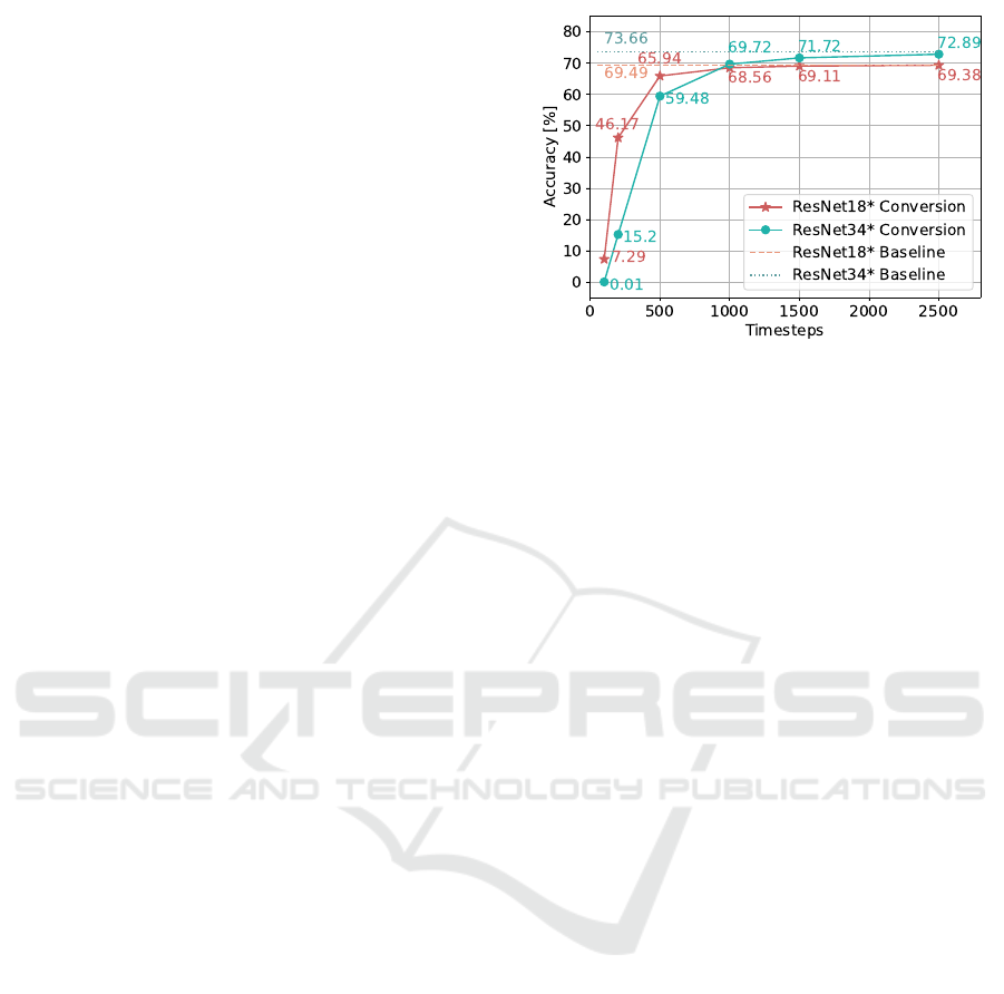
Figure 2: Results of the evaluation of the converted SNN for

the pre-trained networks ResNet18* and ResNet34* using

different numbers of time steps.

Our work puts its focus on the comparison of

the basic concepts and limitations behind different

training methods for SNNs and evaluates their po-

tential applicability in future real-world scenarios,

which does not only depend on the achieved accu-

racy. For this reason, we will use basic algorithms,

that showcase the general advantages and disadvan-

tages of the direct training of SNNs and the conver-

sion based on ANNs. For the direct training method,

we therefore use gradient descent and overcome the

non-differentiability of the spiking neuron formula-

tion by using the arctangent as a surrogate gradient

during the backward pass. To convert the trained

ANN into a SNN, we use the algorithm by Rueck-

auer et al. (2017). It addresses the handling of batch

normalization, whose parameters can be absorbed in

other parameter layers. In addition, the weights and

biases of the ANN are normalized by the maximum

output tensor of each layer.

3.3 ANN to SNN Conversion

In Figure 2 it can be seen that the accuracy after con-

version depends considerably on the number of time

steps t used for the simulation of the converted SNN.

After 100 time steps, the converted networks can only

achieve about 10 percent of the performance of the

original ANN for Resnet18*. For the deeper network

Resnet34*, the converted SNN is almost not able to

perform any classiﬁcation after 100 steps. This shows

that the deeper the network architecture is, the more

accurate the approximations of the ﬂoating point val-

ues of the ANN must be. Accordingly, more time

steps for the rate coding are necessary to achieve a

certain performance. Only after 1000 time steps are

the converted SNNs able to reach a similar accuracy

compared to the baselines of the pre-trained ANNs.

ICPRAM 2023 - 12th International Conference on Pattern Recognition Applications and Methods

470

Table 1: Top-1 classiﬁcation accuracy on the ImageNet

evaluation dataset for the directly trained and converted

SNNs as well as for the pretrained ANNs.

Architecture NN type Training t acc1 [%]

ResNet18 ANN direct - 67.00

ResNet34 ANN direct - 70.70

ResNet18* ANN direct - 69.93

ResNet34* ANN direct - 73.66

ResNet18 SNN direct 5 47.99

ResNet18 SNN direct 10 53.51

ResNet34 SNN direct 5 44.73

ResNet34 SNN direct 10 52.71

ResNet18* SNN conversion 2500 69.38

ResNet34* SNN conversion 2500 72.89

However, the loss of performance compared to the

original network becomes negligible with 2500 time

steps. It can be seen that there is an exponential rela-

tionship between the number of time steps and the ac-

curacy. Nonetheless, the goal of the conversion meth-

ods is the approximation of the original ANN and will

thus most likely result in a reduced performance for

the SNN.

3.4 Direct Training vs Conversion

Table 1 shows the comparison of the results for the

original ANNs, the converted SNNs and the directly

trained SNNs. In this case, it can also be seen that re-

moving the maxpooling layer actually increases the

performance of the networks. Accordingly, the re-

sults from the conversion based on the Resnet18* and

ResNet34* architectures are not directly comparable

to the directly trained SNNs, which all contain the

maxpooling layer as in the original architecture.

The directly trained SNNs with t = 5 have about

20 percentage points lower accuracy than the original

networks, since the networks are very deep and the

error of the surrogate gradient adds up across the lay-

ers. However, for the directly trained ResNet18 and

ResNet34 with t = 10, the performance increases sig-

niﬁcantly by about 6 and 8 percent, respectively, com-

pared to their training runs with 5 time steps, which

shows that a higher number of time steps leads to an

increased performance.This is due the higher number

of potential output spikes, which are produced for ev-

ery time step and help distinguishing similar classes.

Moreover, the resulting gradient becomes more mean-

ingful, since the behavior of all neurons is considered

over all time steps. Thus, there is further potential for

direct training if the number of time steps is increased

even further, especially for deeper architectures.

The results of the conversion with t = 2500 are

clearly superior compared to the directly trained

SNN. However, as evident from Figure 2, for the con-

versions of the ResNet18* and Resnet34* architec-

ture about 200 and 500 time steps, respectively, are

necessary to achieve similar results to the directly

trained SNNs. Therefore, the conversion methods re-

sult in a latency that is about two orders of magnitudes

higher compared to the direct training.

4 DISCUSSION

Training SNNs is still a challenging task, especially

for deep and complex network architectures. Biologi-

cal algorithms such as STDP currently handle only lo-

cal updates based on the correlation of the behaviors

of neighboring neurons. Since no end-to-end train-

ing of SNNs is possible in this way, the error is prop-

agated and accumulated through all network layers.

This makes it impossible to train deep state-of-the-

art network architectures. Nonetheless, there is great

potential in the biological approach, as it can lead to

more understanding of the brain’s processes.

However, until the global training processes in

the brain are discovered, direct training of SNNs is

the best option. Direct training takes into account

the temporal component of spikes and thus exploits

their true potential. This makes them particularly at-

tractive for applications with event-based data, since

they allow an asynchronous and sparse input with

which traditional ANNs have to struggle. The only

problem is the discontinuity in the spiking function,

which prevents gradient descent from being applied

directly. However, this can be solved by approximat-

ing the gradient by a surrogate function, especially

since it has been shown that even random feedback in

small networks leads to good results (Lillicrap et al.,

2016). Furthermore, the direct training of SNNs is the

only method, which has the future potential to fully

take advantage of neuromorphic chips for inference

as well as for training. This is relevant in terms of

energy efﬁciency in the whole process of creating ap-

plications of SNNs in real world scenarios. On syn-

chronous hardware such as GPUs, simulated training

of SNNs tends to have increased energy consumption

due to the multiple time steps over which spikes are

fed into the network.

The inherent temporal component of spiking data

cannot be exploited in a conversion from ANNs to

SNNs, since the ANN must be trained on synchronous

hardware and further struggles with very sparse in-

puts. Moreover, the converted SNN is necessarily

only an approximation of the original ANN with the

goal of increasing energy efﬁciency. However, the

temporal component is completely ignored, so that for

On the Future of Training Spiking Neural Networks

471

example event data cannot be entered directly. Fur-

thermore, other pruning methods are available in or-

der to reduce energy consumption of ANNs, which

means there is no necessity to enforce the constraints

of the SNN architecture in order to reach this goal.

In addition, the original ﬂoating point values must be

approximated by the ﬁring rate during the conversion.

This means, that an enormous latency is required to

achieve a suitable accuracy, which in turn increases

the energy consumption and the inference time ex-

tremely. This makes converted SNNs almost unusable

for complex real world scenarios and direct training of

SNNs should be preferred.

ACKNOWLEDGEMENTS

This work was funded by the Carl Zeiss Stiftung,

Germany under the Sustainable Embedded AI project

(P2021-02-009).

REFERENCES

Adrian, E. D. and Zotterman, Y. (1926). The impulses pro-

duced by sensory nerve endings. The Journal of Phys-

iology.

Andrychowicz, O. M., Baker, B., Chociej, M., J

ozefowicz,

R., McGrew, B., Pachocki, J., Petron, A., Plappert,

M., Powell, G., Ray, A., Schneider, J., Sidor, S.,

Tobin, J., Welinder, P., Weng, L., and Zaremba, W.

(2019). Learning dexterous in-hand manipulation.

The International Journal of Robotics Research.

Arrow, C., Wu, H., Baek, S., Iu, H. H., Nazarpour, K.,

and Eshraghian, J. K. (2021). Prosthesis control us-

ing spike rate coding in the retina photoreceptor cells.

In International Symposium on Circuits and Systems

(ISCAS).

Balasubramanian, V. (2021). Brain power. Proceedings of

the National Academy of Sciences.

Bi, G. and Poo, M.-m. (1998). Synaptic modiﬁcations in

cultured hippocampal neurons: Dependence on spike

timing, synaptic strength, and postsynaptic cell type.

The Journal of Neuroscience.

Brunel, N. and van Rossum, M. C. W. (2007). Lapicque’s

1907 paper: from frogs to integrate-and-ﬁre. Biologi-

cal Cybernetics.

Chen, X., Ma, H., Wan, J., Li, B., and Xia, T. (2017). Multi-

view 3d object detection network for autonomous

driving. In Conference on Computer Vision and Pat-

tern Recognition (CVPR).

Datta, G., Kundu, S., and Beerel, P. A. (2021). Train-

ing energy-efﬁcient deep spiking neural networks with

single-spike hybrid input encoding. International

Joint Conference on Neural Networks (IJCNN).

Dehaene, S. (2003). The neural basis of the weber–fechner

law: a logarithmic mental number line. Trends in Cog-

nitive Sciences.

Deng, J., Dong, W., Socher, R., Li, L.-J., Li, K., and Fei-

Fei, L. (2009). Imagenet: A large-scale hierarchical

image database. In Conference on Computer Vision

and Pattern Recognition (CVPR).

Deng, L., Wu, Y., Hu, X., Liang, L., Ding, Y., Li, G., Zhao,

G., Li, P., and Xie, Y. (2019). Rethinking the per-

formance comparison between snns and anns. Neural

Networks.

Diehl, P. U., Neil, D., Binas, J., Cook, M., Liu, S.-C., and

Pfeiffer, M. (2015). Fast-classifying, high-accuracy

spiking deep networks through weight and threshold

balancing. In International Joint Conference on Neu-

ral Networks (IJCNN).

Gallego, G., Delbruck, T., Orchard, G., Bartolozzi, C.,

Taba, B., Censi, A., Leutenegger, S., Davison, A. J.,

Conradt, J., Daniilidis, K., and Scaramuzza, D.

(2022). Event-based vision: A survey. Transac-

tions on Pattern Analysis and Machine Intelligence

(TPAMI).

Gerstner, W. and Kistler, W. M. (2002). Spiking Neu-

ron Models: Single Neurons, Populations, Plasticity.

Cambridge University Press.

He, K., Zhang, X., Ren, S., and Sun, J. (2016). Deep resid-

ual learning for image recognition. In Conference on

Computer Vision and Pattern Recognition (CVPR).

Izhikevich, E. (2003). Simple model of spiking neurons.

Transactions on Neural Networks.

Krizhevsky, A. (2009). Learning multiple layers of fea-

tures from tiny images. Technical report, University

of Toronto.

Krizhevsky, A., Sutskever, I., and Hinton, G. E. (2012). Im-

agenet classiﬁcation with deep convolutional neural

networks (neurips). In Neural Information Process-

ing Systems.

Lecun, Y., Bottou, L., Bengio, Y., and Haffner, P. (1998).

Gradient-based learning applied to document recogni-

tion. Proceedings of the IEEE.

Li, H., Liu, H., Ji, X., Li, G., and Shi, L. (2017). Cifar10-

dvs: an event-stream dataset for object classiﬁcation.

Frontiers in Neuroscience.

Lillicrap, T. P., Cownden, D., Tweed, D. B., and Akerman,

C. J. (2016). Random synaptic feedback weights sup-

port error backpropagation for deep learning. Nature

Communications.

Maass, W. and Markram, H. (2004). On the computational

power of circuits of spiking neurons. Journal of Com-

puter and System Sciences.

Meng, Q., Xiao, M., Yan, S., Wang, Y., Lin, Z., and Luo,

Z.-Q. (2022). Training high-performance low-latency

spiking neural networks by differentiation on spike

representation.

Morris, R. (1999). D.o. hebb: The organization of behavior,

wiley: New york; 1949. Brain Research Bulletin.

Nunes, J. D., Carvalho, M., Carneiro, D., and Cardoso, J. S.

(2022). Spiking neural networks: A survey. IEEE

Access.

Orchard, G., Jayawant, A., Cohen, G., and Thakor, N.

(2015). Converting static image datasets to spiking

ICPRAM 2023 - 12th International Conference on Pattern Recognition Applications and Methods

472

neuromorphic datasets using saccades. Frontiers in

Neuroscience.

Rathi, N., Srinivasan, G., Panda, P., and Roy, K. (2020).

Enabling deep spiking neural networks with hybrid

conversion and spike timing dependent backpropaga-

tion. International Conference on Learning Represen-

tations (ICLR).

Rueckauer, B., Lungu, I.-A., Hu, Y., Pfeiffer, M., and Liu,

S.-C. (2017). Conversion of continuous-valued deep

networks to efﬁcient event-driven networks for image

classiﬁcation. Frontiers in Neuroscience.

Rumelhart, D. E., Hinton, G. E., and Williams, R. J. (1986).

Learning representations by back-propagating errors.

Nature.

Sengupta, A., Ye, Y., Wang, R., Liu, C., and Roy, K. (2019).

Going deeper in spiking neural networks: VGG and

residual architectures. Frontiers in Neuroscience.

ockl, C. and Maass, W. (2021). Optimized spiking neu-

rons can classify images with high accuracy through

temporal coding with two spikes. Nature Machine In-

telligence.

Thompson, N. C., Greenewald, K., Lee, K., and Manso,

G. F. (2021). Deep learning’s diminishing returns:

The cost of improvement is becoming unsustainable.

IEEE Spectrum.

Vaswani, A., Shazeer, N., Parmar, N., Uszkoreit, J., Jones,

L., Gomez, A. N., Kaiser, L. u., and Polosukhin, I.

(2017). Attention is all you need. In Neural Informa-

tion Processing Systems (NeurIPS).

Werbos, P. (1990). Backpropagation through time: what it

does and how to do it. Proceedings of the IEEE.

Wu, Y., Deng, L., Li, G., Zhu, J., Xie, Y., and Shi, L. (2019).

Direct training for spiking neural networks: Faster,

larger, better. AAAI Conference on Artiﬁcial Intelli-

gence (AAAI).

Zenke, F. and Vogels, T. P. (2021). The remarkable ro-

bustness of surrogate gradient learning for instilling

complex function in spiking neural networks. Neural

Computation.

On the Future of Training Spiking Neural Networks

473