Explainability of MLP Based Species Distribution Models: A Case

Study

Imane El Assari

, Hajar Hakkoum

and Ali Idri

1,2 b

ENSIAS, Mohammed V University in Rabat, Morocco

AlKhwarizmi, Mohammed VI Polytechnic University, Benguerir, Morocco

Keywords: Interpretability, xAI, Biodiversity, Species Distribution Modelling, PDP, SHAP, Machine Learning.

Abstract: Species Distribution models (SDMs) are widely used to study species occurrence in conservation science and

ecology evolution. However the huge amount of data and its complexity makes it difficult for professionals

to forecast the evolutionary trends of distributions across the concerned landscapes. As a solution, machine

learning (ML) algorithms were used to construct and evaluate SDMs in order to predict the studied species

occurrences and their habitat suitability. Nevertheless, it is critical to ensure that ML based SDMs reflect

reality by studying their trustworthiness. This paper aims to investigate two techniques: SHapley Additive

exPlanations (SHAP) and the Partial Dependence Plot (PDP) techniques to interpret a Multilayer perceptron

(MLP) trained on the Loxodonta Africana dataset. Results demonstrate the prediction process and how in-

terpretability techniques could be used to explain misclassified instances and thus increase trust between ML

results and domain experts.

1 INTRODUCTION

Environment scientists assert that the magnitude, pace

and severity of the current environmental crisis are

unprecedented (B.Daley and R.Kent, 2005). Several

regions are losing their biodiversity to make way for

human dwelling and industry. Therefore, in order to

safeguard the environment, it’s crucial to implement

well planned policies that take into consideration the

environmental characteristics and biological

outcomes of each region.

As part of the conservation science, having a well-

thought-out strategy for managing the environment

requires a thorough understanding of its components,

namely its climatic conditions and species distribu-

tion. However, it’s hard to pinpoint the exact loca-

tion of each individual of each species at any moment.

Therefore, species distribution models (SDMs) are

used to find whether a species is likely to be present or

absent in a geographic location based on its environ-

mental conditions. Their objective is to understand a

particular ecosystem, its number of species, the com-

position of its population, and to predict the spatial

and temporal pattern of species occurrence.

http://ensias.um5.ac.ma

https://msda.um6p.ma/home

The new technologies and the data they gener- ate

hold great potential for large-scale environmental

monitoring, however traditional statistical approaches

limits its usage which inefficiently distill data into rel-

evant information (D.Tuia et al., 2022). Conversely,

data science community works to apply information

technologies to gather, organize, and analyze biolog-

ical data (American Museum of Natural History, ).

Basically, they try to use machine learning (ML) to

discover new insights and patterns from all the avail-

able expeditions and remote sensing data. ML tech-

niques are useful to perform predictive analytics since

it gives a variety of tools to support complex data

structures, and thus provides a powerful approach for

assessing SDMs challenges. However, according to a

review made by Beery et al. despite the considerable

use of ML techniques in ecology, SDMs has received

relatively little attention from the computer science

community (S.Beery et al., 2021).

In fact, ML contributed to this field in a cou-ple

of areas, namely climate models that repre- sent our

understanding of Earth and climate physics (Rolnick

et al., 2019), forest management based on satellite

imagery and 3D Deep Learning tech- niques(Liu et

690

El Assari, I., Hakkoum, H. and Idri, A.

Explainability of MLP Based Species Distribution Models: A Case Study.

DOI: 10.5220/0011745300003393

In Proceedings of the 15th International Conference on Agents and Artiﬁcial Intelligence (ICAART 2023) - Volume 3, pages 690-697

ISBN: 978-989-758-623-1; ISSN: 2184-433X

 2023 by SCITEPRESS – Science and Technology Publications, Lda. Under CC license (CC BY-NC-ND 4.0)

al., 2021), mapping wetlands distribu- tion in highly

modified coastal catchments (Wen and Hughes,

2020),urban vegetation(Abdollahi and Prad- han,

2021)and many more.

There are two categories of ML algorithms: legi-

ble white-box algorithms that provide readable rules

(SEON, 2022), , and black-boxes which are opaque

yet more powerful since they can identify nonlinear

relationships in data. To remedy this limitation, in-

terpretability attempts to explain model predictions to

understand the reasoning behind the prediction pro-

cess (AI, 2020), avoid bias and gain trust whether

globally or locally. Global interpretability, exam- ines

a model’s general behavior, whereas local inter-

pretability concentrates on a particular scenario that

was supplied as input to the model.

Interpretability techniques have been used to im-

prove the explainability of ML based species distri-

bution models. For instance, Ryo et al. investi- gated

explainable AI (xAI) techniques in the context of

SDMs based on the African elephant dataset (Ryo et

al., 2021). They used random forest (RF) as a black

box algorithm to predict the presence/absence val-

ues of the studied species. In terms of interpretabil-

ity, they used: (1) feature permutation importance

(FI) and the (2) Partial Dependence Plot (PDP) as

global interpretability techniques, FI classifies the

predictor variables according to their importance,

while PDP demonstrate the marginal effect a feature

may have on the ML model predicted outcome

(Molnar, 2019), along with (3) Local Interpretable

Model-Agnostic Explanation (LIME) (Ribeiro et al.,

2016) as a local interpretability technique. According

to this study, the most relevant feature based on FI

was the precipi- tation of the wettest quarter.

This article aims to evaluate and interpret a basic

Multilayer Perceptron (MLP) model trained to fore-

cast the African elephant distribution (GBIF, 2021)

using: (1) the SHapley Additive exPlanations (SHAP)

(Lundberg and Lee, 2017), a local interpretability

method that explains individual predictions based on

the game theoretically optimal Shapley values; and

(2) the Partial Dependence Plot (PDP): a global inter-

pretability technique that visualizes the marginal ef-

fect of an individual feature to the predictive value of

the studied model (Molnar, 2019). This paper an-

swers and discusses the following research questions:

• RQ1: What is the overall performance of the

con- structed MLP models?

• RQ2: What is the local interpretability of the

best performing model?

• RQ3: How global interpretability enhances

local explanations?

The main contributions of this study are the fol-

lowing:

• Assessing and comparing the performance of

12 MLP based classifiers that were

generated by combining 3 different

Hyperparameters using GridSearch.

• Interpreting 3 randomly chosen instances

locally using SHAP and comparing them with

their true labels.

• Explanation of misclassified instances using

PDP.

The remainder of this paper is organized as fol-

lows: Section2 introduces explainable AI and the

difference between Global and Local Interpretability.

Section 3 describes the used dataset and performance

metrics to select the best performing model. Section4

presents the experimental design followed during this

study. A discussion about the obtained results and

findings is presented in Section 5. Section 6 covers

the threats to validity and the conclusion.

BACKGROUND

This section presents the feed-forward neural net-

work used in this research, along with the used in-

terpretability techniques namely SHAP and PDP.

2.1

Artificial Neural Networks: MLP

ANNs are a collection of simple computational units

interlinked by a system of connections (Cheng and

Titterington, 1994) that were inspired from the

brain’s neuron architecture. They are frequently used

in data modelling, as they are perceived as better

substitute to standard nonlinear regression or cluster

analysis prob- lems (Gurney, 1997).

In general, ANNs are organized in layers and this

is where the MLP comes in, it is a typical example of

the feed-forward ANN where information travels in

one direction from input to output (Hakkoum et al.,

2021). A MLP is constituted of 3 types of layers: the

input layer, which receives the data to be processed,

one or more hidden layers, which together constitute

the network’s true engine, and the output layer.

As to optimize the MLP Hyperparameters tuning

phase, GridSearch a technique that specifies a search

space as a grid of Hyperparameters and evaluates ev-

ery position in the grid (Brownlee, 2020)was used.

Explainability of MLP Based Species Distribution Models: A Case Study

691

Table 1: Bioclimatic variables.

Variable Description Abbreviations Range

Elev Elevation Elev [-61 ; 3508]

Bio1 Annual Mean Temperature AMT [7,810688 ; 29,427000]

Bio2 Mean Diurnal Range MDR [6,640182 ; 18,048876]

Bio3 Isothermality (BIO2/BIO7) (×100) Isothermality [26,918064 ; 92,384308]

Bio4 Temperature Seasonality TempSeasonality [15,199914;1039,296265]

Bio5 Max Temperature of Warmes

Month MaxTempWM [17,118000;41,708752]

Bio6 Min Temperature of Coldes

Month MinTempCM [-9,583250 ; 22,415842]

Bio8 Mean Temperature of Wettes

Quarte

MeanTempWQ [6,682958 ; 31,448957]

Bio12 Annual Precipitation AnnualPrecip [3,000000 ; 3369,000000]

Bio13 Precipitation of Wettes

Month PrecipwettestM [1,000000 ; 535,000000]

Bio14 Precipitation of Dries

Month PrecipDriestM [0,000000 ; 105,000000]

Bio15 Precipitation Seasonality PrecipSeasonality [12,457452 ; 153,643448]

Bio18 Precipitation of Warmes

Quarte

PrecipWQ [0,000000 ; 728,000000]

Bio19 Precipitation of Coldes

Quarte

PrecipCQ [0,000000 ; 948,000000]

2.2

Interpretability

Interpretability is determined by whether the model

has a transparent process that allows the users to un-

derstand how inputs are mathematically mapped to

outputs (Doran et al., 2017). It represents the degree

to which a human can consistently predict the model’s

result, and evaluate the forecasting process by giving

the relative importance of each variable.

Interpretability methods can be categorized ac-

cording to various criteria, depending on how they are

used: Intrinsic/ post-hoc; model-specific/ model-

agnostic; global/ local (Molnar, 2019). Global inter-

pretability describes how the entire model behaves,

meanwhile local interpretability focuses on the pre-

diction of a particular instance; it is similar to a zoom

in on a single instance and then examining the reasons

behind the model’s prediction for this input.

This paper uses SHAP to examine the local inter-

pretability of the best performing MLP model. It ex-

plains the model’s individual predictions using Shap-

ley values, a cooperative game theory concept that

calculates the contribution of each feature to the dif-

ference between the predicted value and the aver- age

of all predictions. Shapley values compute the

marginal contribution of each feature to the end out-

come by perturbing the input features and observ- ing

how these changes correspond to the final model

prediction. The Shapley value is then calculated by

taking the average of all marginal contributions

(Gopinath and Kurokawa, 2021). SHAP is a model-

agnostic method, meaning that SHAP’s process re-

main the same regardless of the used ML algorithm.

In addition to SHAP, PDP was used to study the

marginal effect a feature may have on the target vari-

able. It shows whether the relationship between the

target and a feature is linear, monotonic or more com-

plex(Molnar, 2019).

DATA DESCRIPTION AND

PERFORMANCE CRITERIA

The following section describes the used datasets, and

introduces the performance measures.

3.1

Data Description

To run a SDM, two types of data are needed:

occurrence data, which presents the coordinates of the

locations where the studied species occurs, and

environ- mental data, that describes the bioclimatic

conditions of those locations (EcoCommons, 2022).

For occurrence data GBIF LoxodontaAfricana

tabular data were used. It contains 10494 rows and

257 columns, its relevant features are decimal Lon-

gitude, decimal Latitude and the occurrenceStatus.

The decimal longitude and latitude define the species

geographical locations, while the occurrenceStatus

presents the occupancy / absence values at those lo-

cations.

The original record contains 10466 row of pres-

ence data and 28 row of absence data. To resolve this

imbalanced data problem a sample of 8019 back-

ground points were randomly generated using dismo

package in R to sum up with 16511 occurrences of

which 8979 are presence data and 8019 are pseudo-

absences.

Despite the existence of different methods

to generate background points, the randomly

selected pseudo-absences yielded the most reliable.

distribution models (Barbet-Massin et al., 2012).

ICAART 2023 - 15th International Conference on Agents and Artiﬁcial Intelligence

692

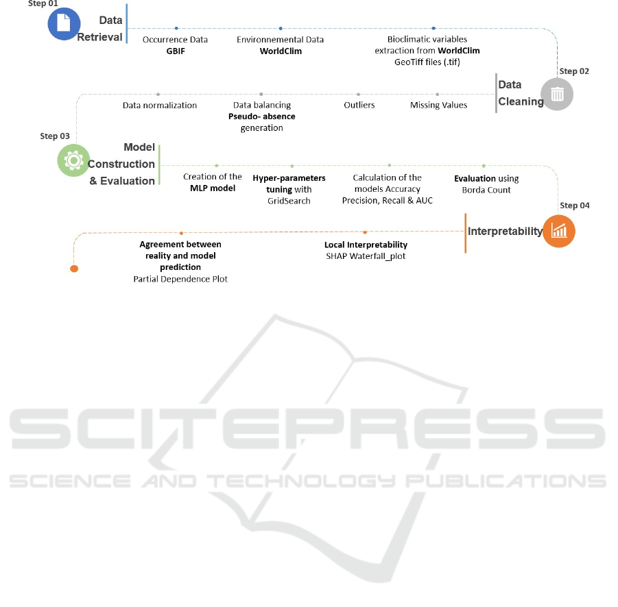
Figure 1: Experimental Design.

It is critical to consider the credibility of the generate

background points, a location with no occurrences of

the species does not imply the absence of the species

in this loca- tion, it could be an area with no data or a

location out of land. To avoid such problems the

dismo package provides different methods dedicated

to SDMs challenges, such as sampling the random

points from a study area to form the pseudo-absences

afterwards or using a mask to exclude the areas not on

land (Spatial Data Science, 2021).

For the environmental data, the WorldClim stan-

dard bioclimatic variables were extracted from 19

GeoTiff (.tif) file using ‘biovars’ function in the dismo

R package. Table1 presents the used bioclimatic vari-

ables and how they were encoded in this work.

3.2

Performance Criteria

The MLP based models performance is reported and

compared in terms of 4 different metrics: Accuracy,

Precision, Recall, and AUC. After calculating these

metrics, the Borda Count, a ranked voting technique

that ranks the models in order of preference, was used

to select the best MLP classifier using the accuracy,

precision, recall, and AUC metrics as voters (Lipp-

man, ).

EXPERIMENTAL DESIGN

This section describes in details the steps followed in

this case study. It starts with model configuration and

selection, then the local interpretation using SHAP’s

Waterfall plots, and finally the PDP plots generation.

The steps are showed in detail in Figure1.

4.1

Data Retrieval and Cleaning

As mentioned in section 3, this study used two types

of data: Loxodonta Africana occurrence data from

GBIF and environmental data from WorldClim, which

were concatenated using R based on their com- mon

geographic points. Missing values, outliers, data

balancing, and normalization were all resolved during

the Data Cleaning phase.

4.2

Models Construction

The MLP classifiers were built using one hidden

layer. Three different hyper-parameters were used to

control the model’s learning process: the batch size,

which represents the number of samples processed

before the model is updated, the solver for weight op-

timization where SGD refers to Stochastic Gradient

Descent, known as the most basic form of gradient

descent while ‘Adam’ is an extension to SGD that

provides faster results (Brownlee, 2017) , however

different studies argue that although Adam converges

faster, SGD generalizes better than Adam and thus

results in improved final performance (Park, 2021).

Finally, we have the hidden layer size that represents

the number of hidden nodes on the first hidden layer,

its selected range was chosen as to provide good

performance but without requiring a huge amount of

time in the training phase since the aim of this

empirical evaluation was interpretability and not

performance.

Explainability of MLP Based Species Distribution Models: A Case Study

693

GridSearch was employed to optimize the Hyper-

parameter tuning phase with 10 cross validation

train

ing. Table 2 presents the used configuration. Note

that

the hidden layer sizes were selected based on

previous experimentations where the highest

performance scores were found close to the mentioned

range in table 2. The batch size and the solver values

were chosen as a standard configuration commonly

found in literature.

Table 2: Hyperparameters configuration.

perparameters Selected Ran

Hidden La

Size [(20,),(25,),(30,)]

Batch size (32,64)

Solve

[’s

d’, ’adam’]

4.3

Interpretability

This step tries to interpret the MLP classifier results

locally using SHAP’s waterfall plot. It explains a set

of 3 different instances that were randomly selected

in a way to have one true positive where the model

agrees with reality and predicts a high habitat suit-

ability, one true negative where the model accurately

predicts a low habitat suitability and one false nega-

tive, where the classifier predicts low habitat suitabil-

ity, while it’s not the case in reality.

After the interpretability of the MLP classifier

PDP was used to determine if there is an agreement

between the classifier predictions, the instances true

label and local interpretability results, PDP plots were

generated for the 2 first ranked features.

RESULTS AND DISCUSSION

This section presents and discusses the results of this

empirical study, namely the models performance, and

interpretability results.

5.1

Models Evaluation

The Hyperparameters combination gave 12 MLP

classifiers. Table 3 describes the overall performance

of the 3 first and the last ranked MLP models accord-

ing to the Borda Count method using accuracy, pre-

cision, recall, and AUC as voters. The classifiers are

presented according to their assigned ranks. Accord-

ing to Table 3, the top-ranked model has 25 neurons in

its hidden layer, 64 as a batch size, which determines

the number of training examples utilized in one iter-

ation (Murphy, 2019), and ’sgd’ as a solver, which

specifies the algorithm weight optimization over the

nodes (Fuchs, 2021). To note that this is the classifier

used in the interpretability phase.

5.2

Local Interpretability

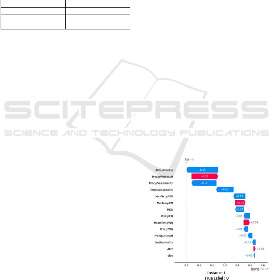
To test the trustworthiness of individual predictions,

a group of 3 instances was randomly chosen, Fig-

ure2 shows their relative SHAP’s waterfall plot ex-

planations. The waterfall plot’s purpose is to show the

SHAP values of each feature as well as its im- pact on

the final prediction. The model’s prediction is

represented in the y-axis by f(x), each bar illustrates

how the feature helps to push the model’s output away

from the base value E(x) that indicates the average of

the model output over training data.

The features with a right arrow influence the pre-

diction more in favor of an appropriate habitat for

African elephants, whilst the features with a left arrow

influence the prediction more in favor of the species’

inadequacy for such environments.

Equation (4) demonstrates how f(x) is calculated.

F(x) = E(x) +

∑

SHAPvalues

(1)

The base value in this study is 0.537, it represents

the average of all observations. The model prediction

for instance 2 is 1 meaning that the studied species can

survive in this location, in this case f(x) is obtained

using Equation (4): 0.536 + 0.01 - 0.02 + 0.02 - 0.03

+ 0.03 + 0.03 + 0.03 + 0.04 - 0.05 + 0.05 + 0.06 +

0.06 + 0.11 + 0.12 = 0.996 1, it sums the base value

E(x) with all SHAP values, the same process is true

for the other instances.

Figure 2: Instance 2 SHAP’s waterfall plot.

ICAART 2023 - 15th International Conference on Agents and Artiﬁcial Intelligence

694

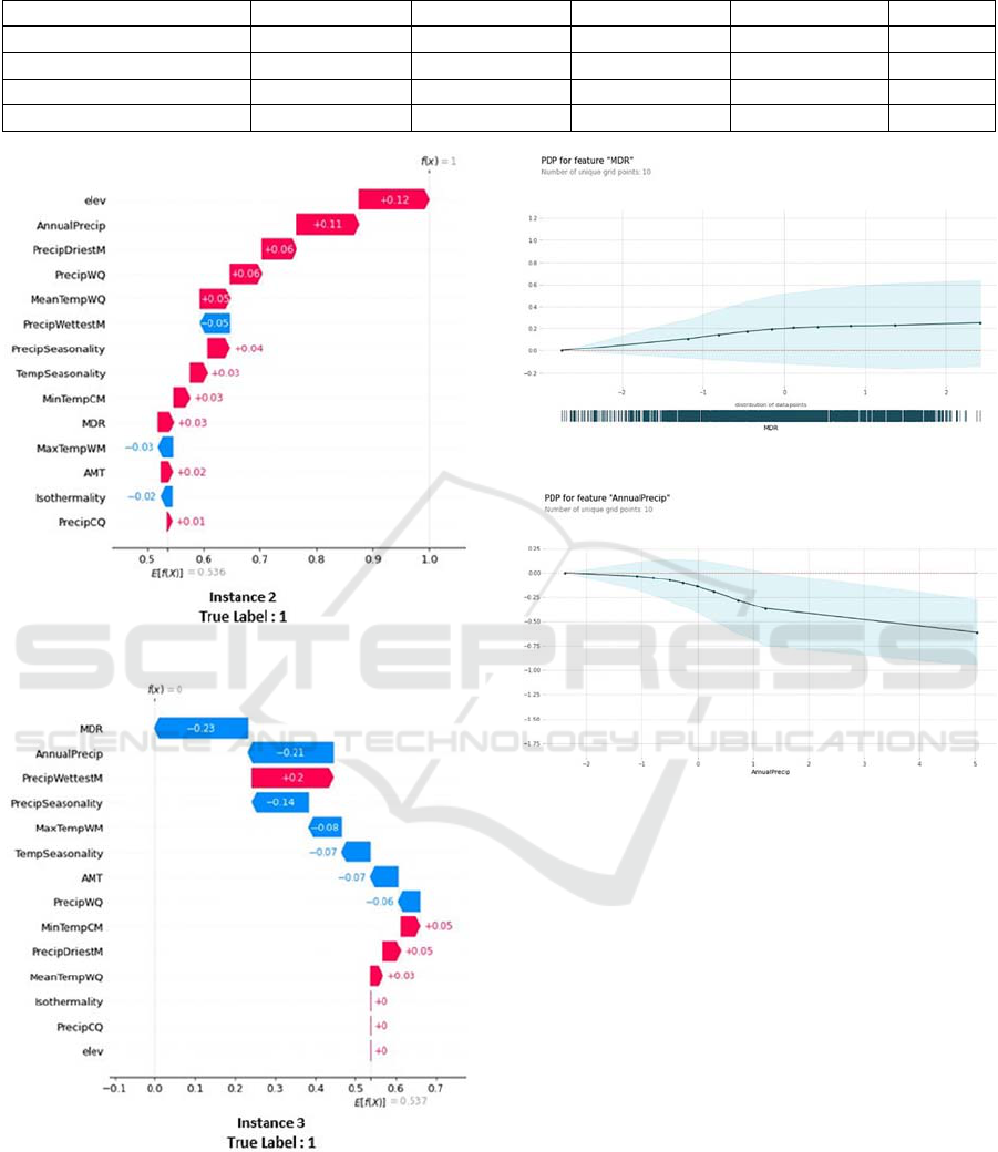
Table 3: Borda Count Results.

MLP Accuracy Precision Recall AUC Ran

[(25,),sgd,64] 0.857059 0.8576 0.856452 0.924786

[(30,),adam ,64] 0.854046 0.854450 0.853481 0.923254

[(30,),sgd,64] 0.851284 0.851420 0.850775 0.920037

[(25,),adam,32] 0.815967 0.816859 0.814878 0.889776 12

Figure 3: Instance2 SHAP’s waterfall plot.

Figure 4: Instance 3 SHAP’s waterfall plot.

In the first instance (Figure 2), the classifier pre-

dicts a low habitat suitability for the location in

question which was mainly proven by SHAP since

f(x) =0 and the ’AnnualPrecip’ variable was ranked

the first among all other variables with a SHAP value

Figure 5: ‘MDR’ Partial Dependence Plot.

Figure 6: ‘Annual Precip’ Partial Dependence Plot.

of -0.25. For instance 2 (Figure 3), the MLP classifier

pre-dicts a high habitat suitability f(x)=1.It was

noticed that according to SHAP the 1st ranked

feature was ‘elev’ which increased the base value

with 12% in comparison with its initial value.

Instance 3 (Figure

4) presents a false negative since the

classifier predicts

a low habitat suitability f(x)=0 while

the true label of the instance is 1 which means that the

models’ prediction affirms the absence of the species

in this location while it is not the case in reality.

In order to gain a deeper understanding of this in-

stance and discover the reasons behind this inaccurate

prediction with the point’s true label, PDP plots were

generated for the first and second ranked features.

Normally ’MDR’ ranges from -3.017 to 2.439, in

this case it is equal to -0.95. According to the PDP

plot in Figure 5, the max reached value at this posi-

tion is less than 0.4, which means that the classifier

predicts a low habitat suitability and that agrees well

with SHAP explanations since f(x) was equal to 0.

Explainability of MLP Based Species Distribution Models: A Case Study

695

The ‘AnnualPrecip’ range is between -2.388 and

5.115, its value in the studied position is approxi-

mately 0.82. According to the PDP plot in Figure 6,

the mean reached value in this point is less than -0.25,

which agrees with SHAP results where f(x) is equal to

0, and explains more why the model predicted a false

0 since both values 0.4 and -0.25 in the PDP plots

(Figure 5 and Figure 6) are far from being around 1.

6 THREATS TO VALIDITY AND

CONCLUSION

This work includes limitations that should be taken

into account when evaluating its findings. During the

data retrieval phase, only one occurrence dataset was

used, incorporating additional data types to the used

tabular dataset may generate better results.

Optimizing the built MLP classifier and creating

more black box models, as well as comparing SHAP

with other global and local interpretability techniques

would undoubtedly provide better explanations to the

misclassified instances.

To conclude, several MLP models were used to

study the distribution of the Loxodonta Africana, the

top performing model was used to predict the species’

occurrence and absence values. Based on SHAP’s re-

sults, the ‘AnnualPrecip’ contributed significantly to

the proposed model’s output since the studied species

lives in the African Savanna known with its tropical

wet and dry climate where rain falls in a single sea-

son and the rest of the year is dry.

SHAP allowed the conduction of models analysis

in depth and leads the selection of appropriate fea-

tures making it a suitable explanation technique for

biodiversity experts to consider when drawing critical

decisions.

Future work would attempt to include more black

box models, and compare their performance as well

as their interpretability with the obtained results using

different techniques such as SHAP’s summary plot,

FI, and LIME.

REFERENCES

Abdollahi, A. and Pradhan, B. (2021). Urban vegeta- tion

mapping from aerial imagery using explainable ai (xai).

Sensors.

AI, I. (2020). What is interpretability? https://www.

interpretable.ai/interpretability/what/.

American Museum of Natural History. Biodiversity

informatics. https://www.amnh.org/research/center- for-

biodiversity-conservation/capacity- development/biodi

versity-informatics.

Barbet-Massin, M., Jiguet, F., Albert, C., and Thuiller, W.

(2012). Selecting pseudo-absences for species distri-

bution models: How, where and how many? Methods in

Ecology and Evolution.

B.Daley and R.Kent (2005). P120 Environmental Science

and Management. London.

Brownlee, J. (2017). Gentle introduction to the adam

optimization algorithm for deep learn- ing. https://ma

chinelearningmastery.com/adam- optimization-algorith

m-for-deep-learning/.

Brownlee, J. (2020). Hyperparameter optimiza- tion with

random search and grid search. https://machinelearn

ingmastery.com/hyperparameter- optimization-with-

random-search-and-grid-search/.

Cheng, B. and Titterington, D. M. (1994). Neural Networks:

Review from a Statistical Perspective. Statistical

Science, 9(1).

Doran, D., Schulz, S., and Besold, T. (2017). What does

explainable ai really mean? a new conceptualization of

perspectives.

D.Tuia, B.Kellenberger, s.Beery, Blair.R.Costelloe, S.Zuffi,

B.Risse, A.Mathis, W.Mathis, M., Langevelde, F.,

T.Burghardt, H.Klinck, R., M.Wikelski, Horn, G.,

D.Couzin, I., M.Crofoot, V.Stewart, C., and T.Berger-

Wolf (2022). Perspectives in machine learning for

widlife conservation. Nature Communications.

EcoCommons (2022). Data for species distribution models.

https://support.ecocommons.org.au/support/solutions/ ar

ticles/6000255996-data-for-species-distribution- models.

Fuchs, M. (2021). Nn - multi-layer perceptron clas- sifier

(mlpclassifier). https://michael-fuchs-python.netlify.ap

p/2021/02/03/nn-multi-layer- perceptron-classifier-mlp

classifier/.

GBIF (2021). Loxodonta africana (blumenbach, 1797).

https://www.gbif.org/fr/species/2435350.

Gopinath, D. and Kurokawa, D. (2021). The shapley value

for ml models. https://towardsdatascience.com/the-

shapley-value-for-ml-models-f1100bff78d1.

Gurney, K. (1997). An Introduction to Neural Networks.

Hakkoum, H., Idri, A., and Abnane, I. (2021). Assessing

and comparing interpretability techniques for artificial

neural networks breast cancer classification. Com-

puter Methods in Biomechanics and Biomedical En-

gineering: Imaging & Visualization.

Lippman, D.Bordacount. https://courses.lumenlearning.

com/ mathforliberalartscorequisite/chapter/borda-count/.

Liu, M., Han, Z., Chen, Y., Liu, Z., and Han, Y. (2021).

Tree species classification of lidar data based on 3d

deep learning. Measurement, 177:109301.

Lundberg, S. M. and Lee, S.-I. (2017). A unified approach

to interpreting model predictions. In Advances in Neu-

ral Information Processing Systems.

Molnar, C. (2019). Interpretable Machine Learn- ing.

https://christophm.github.io/interpretable-ml- book/.

Murphy, A. (2019). Batch size (machine learning).

https://radiopaedia.org/articles/batch-size-machine-lea

rning.

ICAART 2023 - 15th International Conference on Agents and Artiﬁcial Intelligence

696

Park, S. (2021).A 2021 guide to im- proving cnns-

optimizers: Adam vs sgd. https://medium.com/

geekculture/a-2021-guide-to-improving-cnns-optimize

rs-adam-vs-sgd- 495848ac6008.

Ribeiro, M. T., Singh, S., and Guestrin, C. (2016). ”why

should i trust you?”: Explaining the predictions of any

classifier. In Proceedings of the 22nd ACM SIGKDD

International Conference on Knowledge Discovery

and Data Mining. Association for Computing Ma-

chinery.

Rolnick, D., Donti, P. L., Kaack, L. H., Kochanski, K.,

Lacoste, A., Sankaran, K., Ross, A. S., Milojevic-

Dupont, N., Jaques, N., Waldman-Brown, A., Luc-

cioni, A., Maharaj, T., Sherwin, E. D., Mukkavilli,

S. K., Kording, K. P., Gomes, C., Ng, A. Y., Hassabis,

D.,

Platt, J. C., Creutzig, F., Chayes, J., and Bengio, Y.

(2019).

Tackling climate change with machine learn- ing.

Ryo, M., Angelov, B., Mammola, S., Kass, J., Benito, B.,

and Hartig, F. (2021). Explainable artificial in-

telligence enhances the ecological interpretability of

black-box species distribution models. Ecography, 44.

S.Beery, E.Cole, J.Parker, P.Perona, and K.Winner (2021).

Species distribution modeling for machine learning

practitioners: A review. In ACM SIGCAS Conference on

Computing and Sustainable Societies (COMPASS ’21).

Science, S. D. (2021). Absence and background points.

https://rspatial.org/raster/sdm/3

bsencebackground

.html.

SEON (2022). Whitebox machine learning. https://seon

.io/resources/dictionary/whitebox-machine- learning/h-

why-choose-whitebox-over-blackbox-machine-learning.

Wen, L. and Hughes, M. (2020). Coastal wetland mapping

using ensemble learning algorithms: A comparative

study of bag- ging, boosting and stacking techniques.

Remote Sensing.

Explainability of MLP Based Species Distribution Models: A Case Study

697