An Audit Framework for Technical Assessment of Binary Classifiers
Debarati Bhaumik
a
and Diptish Dey
b
Amsterdam University of Applied Sciences, The Netherlands
Keywords: Auditable AI, Multilevel Logistic Regression, Random Forest, Explainability, Discrimination, Ethics.
Abstract: Multilevel models using logistic regression (MLogRM) and random forest models (RFM) are increasingly
deployed in industry for the purpose of binary classification. The European Commission’s proposed Artificial
Intelligence Act (AIA) necessitates, under certain conditions, that application of such models is fair,
transparent, and ethical, which consequently implies technical assessment of these models. This paper
proposes and demonstrates an audit framework for technical assessment of RFMs and MLogRMs by
focussing on model-, discrimination-, and transparency & explainability-related aspects. To measure these
aspects 20 KPIs are proposed, which are paired to a traffic light risk assessment method. An open-source
dataset is used to train a RFM and a MLogRM model and these KPIs are computed and compared with the
traffic lights. The performance of popular explainability methods such as kernel- and tree-SHAP are assessed.
The framework is expected to assist regulatory bodies in performing conformity assessments of binary
classifiers and also benefits providers and users deploying such AI-systems to comply with the AIA.
1 INTRODUCTION
The large-scale proliferation of AI/ML systems
within a relatively short span of time has been
accompanied by their undesirable impact on society
(Angwin, Larson, Mattu, & Kirchner, 2016). For
example, it takes the forms of price discrimination in
online retail based upon geographic location
(Mikians, Gyarmati, Erramilli, & Laoutaris, 2012),
and in unsought societal impact of algorithmic pricing
in tourism and hospitality (van der Rest, Sears,
Kuokkanen, & Heidary, 2022). Often deploying
classification models these systems, due to their
increasing complexity, are often uninterpretable by
humans. The mounting struggle to fully comprehend
the rationale behind decisions made by these systems
(Biran & Cotton, 2017), also fuels the need to
examine and scientifically explain such rationale
(explainability) (Miller, 2019) and approach
explainability in a more structured and actionable
manner (Raji & Buolamwini, 2019; Kazim, Denny, &
Koshiyama, 2021). The need for explainability is
driven among others, by discrimination/biasness
concerns of individuals, ethical considerations of
psychologists and social activists, corporate social
a
https://orcid.org/0000-0002-5457-6481
b
https://orcid.org/0000-0003-3913-2185
responsibility objectives of corporations and the
responsibilities of legislators to protect fundamental
rights of citizens (Schroepfer, 2021; Kordzadeh &
Ghasemaghaei, 2022; Rai, 2022).
Technically assessing AI systems and making
them explainable includes activities such as
validating model assumptions, or generating model
explanations (Miller, 2019). Such activities are very
specific to the choice of algorithms and underlying
model assumptions. Recognizing the importance of
technology-specific approach, our proposed
framework focusses on binary classification
problems. Commonly applied binary classification
models (algorithms) such as logistic regression (LR)
and random forest (RF) are selected. Owing to their
simplicity and their complementary scopes of
application, these algorithms are heavily deployed
(Beğenilmiş & Uskudarli, 2018). LR, when combined
with multilevel models (Gelman & Hill, 2006),
extends the performance of the former considerably.
These MLogRMs are beneficial in circumstances,
where a combination of local behaviour and global
context needs to be accounted for, such as
applications within groups or hierarchies. Our
312
Bhaumik, D. and Dey, D.
An Audit Framework for Technical Assessment of Binary Classifiers.
DOI: 10.5220/0011744600003393
In Proceedings of the 15th International Conference on Agents and Artificial Intelligence (ICAART 2023) - Volume 2, pages 312-324
ISBN: 978-989-758-623-1; ISSN: 2184-433X
Copyright
c
 2023 by SCITEPRESS – Science and Technology Publications, Lda. Under CC license (CC BY-NC-ND 4.0)

proposed audit framework is developed for
application within binary classification problems.
The paper is organized as follows. Section 2
presents a short summary of the AIA. Section 3
presents an audit framework applicable to two
classification models, MLogRM and RF, from a
theoretical perspective highlighting characteristics
that potentially play a role in their audit. Section 5
demonstrates the framework using an online open
dataset. Finally, section 6 presents conclusions with a
view to the future.
2 THE PROPOSED EU AI ACT
Recognizing the roles and concerns of a wide range
of stakeholders, the European Parliament proposed
the AIA (Commissie, 2021), which presents a
conformity regime. Using a tiered risk-based
approach, the AIA defines three tiers, “low- or no-
risk”, “high-risk” and “unacceptable risk”; page 12 of
the Explanatory Memorandum of the AIA defines
these tiers. High-risk systems are subject to ex-ante
conformity assessments and post-market monitoring
systems driven by competence in specific AI
technologies. Although the AIA recognises the
importance of competence, it does not elaborate on
the role competence plays in specific AI technologies;
albeit, “expertise” constitutes one of the 5 key criteria
of a good regulation (Baldwin, Cave, & Lodge,
1999). Furthermore, distinction is made between two
types of high-risk AI systems: stand-alone high-risk
AI systems and those that function as components in
consumer products. The latter are subject to
legislation specific to their inherent sector. On the
former, the AIA stipulates that a provider of a stand-
alone high-risk AI system can choose to conduct ex-
ante conformity assessment internally if its AI system
is fully compliant or use an external auditor if its AI
system is either partially compliant or harmonized
standards governing that AI system is non-existent.
The AIA addresses accountability in the supply
chain and focusses also on AI/ML models that
process data. Aiming to tackle the issues of “remote
biometric identification” and “biometric
categorisation”, the AIA encompasses various
standpoints, among others, prohibited practices,
transparency obligations, governance, and
compliance procedures across the supply chain of
these systems (Bhaumik, Dey, & Kayal, 2022). It
“sets out the legal requirements for high-risk AI
systems in relation to data and data governance,
documentation and recording keeping, transparency
and provision of information to users, human
oversight, robustness, accuracy and security”
(Commissie, 2021, p. 13). Articles 10 to 15 of
Chapter 2 Title III of the AIA elaborates on these
legal requirements.
As legislations evolve towards regulatory
frameworks and eventually result in enforcement
strategies such as in the AIA, the mechanisms
deployed in enforcement play a critical role in the
eventual success of the legislation (Baldwin et al,
1999). In the AIA regime, enforcement activities
would include maintaining registers of high-risk AI
systems and technical audit of such systems.
3 AUDIT FRAMEWORK FOR
TECHNICAL COMPLIANCE
Binary classification is one of the most ubiquitous
tasks required to solve problems in almost every
industry. From default prediction in credit risk to
diagnosing benign or malignant cancer in healthcare
to churn prediction in telecom, binary classifiers are
heavily used for decision making (Kim, Cho, & Ryu,
2020; Esteva, Kupre, Novoa, Ko, Swetter, Blau, &
Thrun, 2017). The task of a binary classifier is to
predict the class (1/0 or yes/no) to which a particular
instance belongs, given some input features, e.g., to
predict if an obligor will default on their loan given
her credit rating, marital status, income, and gender.
With the advent of higher computing power, AI/ML
systems are increasingly deployed for making binary
classification decisions in different domains (Xu, Liu,
Cao, Huang, Liu, Qian, Liu, Wu, Dong, Qiu, & Qiu,
2021; Sarker, 2021). There exists many AI/ML
algorithms of varying complexity to perform binary
classification tasks. Amongst the more commonly
used AI/ML classifiers, LRs, decision trees, K-
nearest neighbors, and MLogRMs are less complex to
construct, whereas RFs, support vector machines,
XGBoost, artificial neural networks, and deep neural
networks have more complex architectures. The
higher the model complexity, the higher its prediction
accuracy. However, this comes at the cost of
explainability of model predictions (Gunning, Stefik,
Choi, Miller, Stumpf, & Yang, 2019).
3.1 Common Binary Classifiers
LR and RF are two commonly used classifiers for
both binary and muti-class classification tasks in
different sectors such as finance, healthcare,
agriculture, IT and many more. Applications range
from credit scoring in finance to diabetes detection in
An Audit Framework for Technical Assessment of Binary Classifiers
313

healthcare, forest fire and soil erosion prediction in
agriculture, cyber security intrusion detection in IT
(Dumitrescu, Hué, Hurlin, & Tokpavi, 2022;
Daghistani & Alshammari, 2020; Milanović,
Marković, Pamučar, Gigović, Kostić, & Milanović,
2020; Ghosh & Maiti, 2021; Gupta & Kulariya,
2016). For the majority of such applications, it is
observed that RF classifiers tend to achieve higher
accuracy compared to LR classifiers. However, this
high accuracy comes at the cost of explainability of
the classifier’s predictions. Therefore, in highly
regulated sectors, such as banking, LR classifiers are
still preferred over the more accurate but more
‘opaque’ RF classifiers (EBA, 2020).
When a dataset has inherent group or hierarchical
structure, the accuracy of LR classifiers can be
increased without losing their explainability power,
by coupling them with multilevel models (MLMs),
resulting in MLogRMs (Gelman & Hill, 2006).
MLogRMs are capable of capturing the individual
level (local) effects while preserving the overarching
group level (global) effects. MLogRMs are used
increasingly in industry across different sectors such
as insurance (Ma, Baker. & Smith, 2021), healthcare
(Adedokun, Uthman, Adekanmbi, & Wiysonge,
2017), agriculture (Giannakis & Bruggeman 2018,
Nawrotzki & Bakhtsiyarava, 2017), and urban
planning (Wang, Abdel-Aty, Shi, & Park, 2015).
Given the high penetration of binary classifiers in
real-world industrial applications, it is important that
these classifiers are implemented in a trustworthy
manner. Fairness and transparency are two commonly
used attributes of a trustable system/model. Fairness
can be achieved through detection and avoidance of
biases in these systems, which can otherwise,
potentially lead to discrimination of minorities and
unprivileged groups (Mehrabi, Morstatter, Saxena,
Lerman, & Galstyan, 2021). Bias could creep into the
classifiers in three phases of their model lifecycle: (i)
pre-processing phase: when model training data is
collected, (ii) in-processing phase: when the
algorithm of the classifier is being trained on the
collected data, and (iii) post-processing phase: when
the model is in production and is not monitored for
model re-training. Therefore, it is not only important
to have technical expertise for bias detection, but also
process expertise, to ensure procedures are in place
for bias mitigation. Transparency is the other attribute
of a trustable system. In case of binary classifiers this
implies that the predictions made by the classifier can
be explained to various stakeholders, such as, model
developers, model users, and end users.
This paper is incremental and builds upon the
audit framework applied to MLogRM by Bhaumik et
al (2022). For the sake of completeness of the
framework, this paper repeats some of their
conclusions. This paper is innovative in two ways:
firstly, it extends their audit framework and
introduces additional sub-aspects such as robustness
and accuracy of counterfactual explanations and
secondly, it applies the audit framework to go beyond
MLogRMs and include RFMs.
3.2 Multilevel Logistic Regression
As stated earlier, MLogRMs are used in binary
classification problems where data is structured in
groups or is characterized by inherent hierarchies.
MLogRMs can be perceived as a collection of
multiple LR models that vary per MLM group. These
multiple LR models are modeled using random
variables with a common distribution. Therefore, the
model parameters (coefficients) of MLogRMs vary
per MLM group but they come from a common
distribution. The common distribution of the model
parameters leads to higher predictive power
compared to simple LR models. MLogRMs come in
three flavors: (i) random intercept model, where only
the intercepts vary per MLM-group, (ii) random slope
model, where only the slopes vary per MLM-group,
and (iii) random intercept and slope model, where
both the intercepts and the slopes vary per MLM-
group (Gelman and Hill, 2006). Equation 1 presents
of a simple random intercept and slope MLogRM
model with three independent variables 𝑥

,𝑥

,𝑥

and
a dependent variable 𝑦:
log
ℙ
(
𝑦

=1
)
ℙ
(
𝑦

=0
)
=𝛼
[

]

+ 𝛽
[

]


𝑥


+𝛽
[

]


𝑥


+𝛽


𝑥


+ 𝜖

.
(1)
In equation (1), 𝑖=
{
1,…,𝑁
}
, 𝑁 being the total
number of data points, 𝑗=
{
1,…,𝐽
}
, 𝐽 being the
number of MLM-groups. Model assumptions
represented in equation (1) include:
- log

ℙ
(


 
)
ℙ
(


 
)

, the log-odds term, has a linear
relationship with the independent variables 𝑥

’s.
- 𝑥′𝑠, the independent variables, are mutually
uncorrelated.
-
𝜖


𝑠 , the error terms, are normally distributed
with mean zero.
- The varying intercept 𝛼
[

]
and slope 𝛽
[

]
terms
follow normal distributions.
- The training and testing datasets follow the
same distribution.
These assumptions lead to the following statistical
properties for the model in equation (1):
ICAART 2023 - 15th International Conference on Agents and Artificial Intelligence
314

- 𝜖

∼𝒩0, 𝜎


,
- 𝛼
[

]
∼𝒩
(
𝜇

, 𝜎


)
, and 𝛽
[

]
∼𝒩𝜇

, 𝜎


, for
𝑗 = 1,…, 𝐽.
- 𝐷

≜ 𝐷

.
MLogRMs can only capture linear relationship
between independent and dependent variables.
Therefore, predictive power of these models
decreases when there exists a non-linear relationship
between independent and dependent variables.
3.3 Random Forests
RFMs are known to have higher accuracy and
predictive power when compared to LR models. This
is because RFMs can learn non-linear relationships
between the independent and the dependent variables
(Breiman, 2001). A RFM is an ensemble of decision
trees build from different bootstrapped samples of the
training dataset, along with taking a random subset of
the independent variables for each decision tree. A
decision tree is a supervised learning method where
the feature space is partitioned recursively into
smaller regions. The recursive partition of the feature
space is done through a set of decision rules which
typically results in ‘yes/no’ conditions. These
cascading ‘yes/no’ decision rules can be seen as a
tree, hence the name decision tree. The class which
gets the most votes from the ensemble of decision
trees is the final predicted class by the RFM.
The ensembles of decision trees help in reducing
the variance of the classifier, resulting in higher
predictive power. The widespread use of RFMs
in industrial applications is not only due to their high
Table 1: Audit framework for technical assessment.
Aspects Sub-aspects Contributors KPIs
1. Model
Assess that a model
fitted to data is
technically stable and
valid.
1.1 Formulation of relevant
assumptions
Tests are performed to ensure validity
of model assumptions and statistical
properties.
Model assumptions 1.1.1 Presence in
technical
documentation
Statistical properties 1.1.2a VIF
1.1.2b SWT
1.1.2c BPT
1.2 Accuracy of predictions
Checks are undertaken to monitor
accuracy of model predictions.
Discriminatory power 1.2.1 AUC-ROC
Predictive power 1.2.2 F1-score
1.3 Robustness
Tests are conducted to assess
sensitivity of model output.
Sensitivity of model output to
change in model parameter
1.3.1 TSVR
Sensitivity of input around
inflection points
1.3.2 CSVP
2. Discrimination
Assess that a model is
fair at individual and
group levels.
2.1 Group fairness
Tests are performed to check if group
fairness for equal group treatment is
within an acceptable range.
Predicted versus actual outcome 2.1.1 EqualOdds
Predicted equality 2.1.2a DI
2.1.2b SP
2.2 Individual fairness
Tests are performed to check if
individual fairness for equal
treatment of individuals is within an
acceptable range.
Intra-group fairness 2.2.1 Diff
Ind
Inter-group fairness 2.2.2 Diff
Ind_GRP
3. Transparency &
explainability
Assess the extent to
which model
predictions are
explainable to
humans and suggest
actions that would
facilitate a
(alternative) desirable
prediction.
3.1 Accuracy of feature attribution
explainability methods
Tests are performed to assess quality
of feature attribution explainability
methods used to explain model
predictions to humans.
Feature contribution order 3.1.1 ρ
order
Aggregated feature contribution
(because individuals cannot be
compared)
3.1.2 PUX
Feature contribution sign 3.1.3 POIFS
3.2 Accuracy of counterfactual
explanations
Tests are performed to assess quality
of counterfactuals generated to
substantiate a model output.
Percentage of valid
counterfactuals
3.2.1 PVCF
Proximity 3.2.2 PCF
Sparsity 3.2.3 SCF
Diversity 3.2.4 DCF
An Audit Framework for Technical Assessment of Binary Classifiers
315

predictive power but also due to their inbuilt global
variable importance measure (VIM) for the
independent/feature variable. This makes RFMs more
explainable at the global level unlike other ‘black-
box’ models. However, the global VIM fails to
explain local or instance-based predictions. A new
methodology, dimensional reduction forests,
formulated by Loyal, Zhu, Cui, & Zhang (2022) can
provide explanations for local predictions. However,
the method is not performance tested against the
commonly used feature attribution explanation
methods SHAP and LIME (Molnar, 2020).
Being non-parametric in nature, RFMs do not
have any distributional assumptions. However, for
unbiased model performance metrics calculations, it
is important that both the training and test datasets
follow the same distribution i.e., 𝐷

≜ 𝐷

.
3.4 Framework for Technical Audit of
Classification Models
As discussed in the sections 3.2 and 3.3, technical
assessment of binary classifiers would require
assessing various algorithmic aspects. These include:
(i) model aspects, (ii) discrimination aspects, and (iii)
transparency & explainability aspects, which are
presented in our proposed audit framework (Table 1).
The following sections of this paper present various
sub-aspects, contributors and their corresponding
KPIs for assessing these algorithmic aspects.
3.4.1 KPIs for Model Assumptions and
Statistical Properties
The KPI associated with assessing model
assumptions is qualitative as it is assessed by the
extent of their presence in technical documentation.
The KPIs for assessing statistical properties
presented in Table 1 are variance inflation factor
(VIF), Shapiro-Wilk test (SWT) and Breusch-Pagan
test (BPT). VIF measures the presence of multi-
collinearity among independent variables and a value
of VIF > 5.0 should be mitigated. SWT is a statistical
test which is used to check normality in data. For
MLogRM this test is applied to check if model
residuals are normally distributed. Results of
MLogRM can be trusted only if residuals of a fitted
model have constant variances. This assumption is
checked using BPT that checks for heteroscedasticity
in data samples. For both SWT and BPT if p-values
are close to zero, then the null hypothesis of normality
and constant variance in sample data is rejected in
favour of the alternative hypothesis.
3.4.2 KPIs for Accuracy of Predictions
The KPIs associated with measuring the sub-aspect
accuracy of predictions are Area under the ROC
curve (AUC-ROC) and F1-score. F1-score measures
the predictive power and is the geometric mean of
precision and recall of a binary classifier. Whereas,
AUC-ROC, measures how good a binary classifier is
in separating the two classes (i.e., the discriminatory
power). Both of these KPIs take values between [0,1]
and the closer their values are to 1, the more accurate
the binary classifier is.
3.4.3 KPIs for Robustness
To assess the robustness of a model, two contributors
have been proposed, sensitivity of the model output to
change in model parameter and sensitivity of input
around the inflection points. The KPIs proposed to
measure these contributors are total Sobol’s variance
ratio (TSVR) and cosine similarity vector pairs
(CSVP) respectively.
TSVR is computed by taking the sum of the first-
order sensitivity indices over all the estimated model
parameters. The first-order sensitivity index, also
known as the Sobol’s variance ratio for the 𝑖

parameter, is a ratio of the variance of a model output
under the variation of a single model parameter (for
example 𝛽

in equation (1)) to the variance of the
model output (Tosin, Côrtes, & Cunha, 2020).
Mathematically,
𝑆

=
𝑉𝑎𝑟



𝑌| 𝜷

,𝑿



𝑉𝑎𝑟
(
𝑌
|
𝜷, 𝑿

)
,
(2)
where, 𝑉𝑎𝑟



𝑌| 𝜷

,𝑿


 is the variance of the
model output in which the 𝑗

parameter is varied
while keeping the other model parameters 𝜷

at
constant and the input independent variables/ feature
values of the test dataset (𝑿

) at their mean values,
i.e., 𝑿


. 𝑉𝑎𝑟
(
𝑌
|
𝜷,𝑿

) is the variance of the
model output on the test dataset 𝑿

and 𝜷 are the
estimated model parameters.
Finally,
𝑇𝑆𝑉𝑅=
∑
𝑆



,
(3)
where, 𝑃 is the total number of estimated model
parameters. For the MLogRM in the case-study there
are 4 model parameters, one corresponding to the
intercept term 𝛼 in equation (1) and the other three
corresponding to the slope terms from age, BMI and
number of children, i.e., 𝛽

,𝛽

and 𝛽

, respectively.
We vary the 𝑗

model parameter 𝛽


between the
ICAART 2023 - 15th International Conference on Agents and Artificial Intelligence
316

interval 𝛽

−𝑆𝐸


,𝛽

+𝑆𝐸


, where 𝑆𝐸


is the
standard error of the estimated model parameter 𝛽

.
A smaller value of TSVR corresponds to a better
model, because the model then is less sensitive under
the variation of parameters. The value of TSVR has an
upper bound of 1 – high order interaction terms. The
higher order interaction terms are non-trivial,
therefore knowing the exact upper bound of TSVR is
difficult, however it cannot exceed the value of 1.
CSVP is the number of input vector pairs
predicted to be in different classes around the
inflection point ( 𝑝 = 0.5) with cosine similarity
greater that 1−𝛿. The inflection point can be seen as
the probability threshold point to classify an input
data point if it belongs to class 0 (for 𝑝<0.5) or class
1 (for 𝑝≥0.5). In simpler terms, CSVP finds the
number of vector pairs that are very similar in values
but have been predicted to be in different classes. This
metric helps in assessing how sensitive are the model
predictions for very similar datapoints around the
point of inflection. For computing CSVP, a
neighborhood of [𝑝 −0.01,𝑝+ 0.01] was
considered around the inflection point and 𝛿=0.1
was taken for cosine similarity. Therefore, only those
vector pairs were chosen around the inflection point,
which had cosine similarity greater than 0.9 and were
predicted to be in different classes. A lower value of
CSVP results in a more robust classifier.
3.4.4 KPIs for Discrimination
As proposed by Pessach & Schmueli (2022) and
Hardt, Price, & Srebro (2016), discrimination can be
assessed through two sub-aspects, group fairness and
individual fairness. The KPIs proposed to assess
group fairness are Statistical Parity (SP), Disparate
Impact (DI) and EqualizedOdds (EqualOdds). SP and
DI measure the difference between the positive
predictions across the sensitive groups 𝑆, such as
gender or ethnicity. These KPIs can be calculated as:
𝑆𝑃= ℙ𝑌

=1𝑆=1−ℙ𝑌

=1𝑆≠1
(4)
and,
𝐷𝐼=
ℙ[𝑌

=1|𝑆=1]
ℙ[𝑌

=1|𝑆≠1]
(5)
In the equations above, 𝑌

=1 represents the
favourable class, S represents the feature or attribute
that is possibly discriminatory, and 𝑆≠1 represents
the under-privileged group. A low value of SP in
equation 4 and a high value of DI in equation 5 imply
that a favoured classification is similar across
different groups. One of the few available
benchmarks for these KPIs is that of an acceptable
value of DI of 0.8 or higher (Stephanopoulos, 2018).
Equalized odds, the mean of differences between
false-positive rates and true-positive rates, is given by
𝐸𝑞𝑢𝑎𝑙𝑂𝑑𝑑𝑠=
1
2
(
𝐷𝑖𝑓𝑓

+𝐷𝑖𝑓𝑓

)
,
(6)
where, 𝐷𝑖𝑓𝑓

is calculated as the absolute value of
the difference between ℙ𝑌

=1𝑆=1,𝑌=0 and
ℙ𝑌

=1𝑆≠1,𝑌=0. 𝐷𝑖𝑓𝑓

is calculated as the
absolute value of the difference between
ℙ𝑌

=1𝑆=1,𝑌=1 and ℙ𝑌

=1𝑆≠1,𝑌=1.
Ideally 𝐸𝑞𝑢𝑎𝑙𝑂𝑑𝑑𝑠 should be zero.
The KPIs proposed to assess individual fairness
are 𝐷𝑖𝑓𝑓

and 𝐷𝑖𝑓𝑓
_
which checks if similar
individuals are treated equally within a MLM-group
and across MLM-groups respectively. 𝐷𝑖𝑓𝑓

is
calculated using the formula
𝐷𝑖𝑓𝑓

=ℙ𝑌

(

)
=𝑦|𝑋
(

)
,𝑆
(

)
−
ℙ𝑌

(

)
=𝑦|𝑋
(

)
,𝑆
(

)
,
𝑖𝑓𝑑
(
𝑖,
𝑗
)
≈0
(7)
where, 𝑖 and 𝑗 denote two individuals with 𝑆 and 𝑋
representing sensitive attributes and associated
features of the individuals respectively, 𝑑
(
𝑖,𝑗
)
is the
distance metrics and its value close of zero ensures
that the two individuals compared are in some respect
similar.
𝐷𝑖𝑓𝑓
_
is calculated by
𝐷𝑖𝑓𝑓

_

=ℙ𝑌

(,)
=𝑦|𝑋
(
,
)
,𝑆
(
,
)

−ℙ𝑌

(,)
=𝑦|𝑋
(
,
)
,𝑆
(
,
)

(8)
where 𝑎 and 𝑏 refer to two different MLM-groups.
The smaller the values of these KPIs, the fairer
similar individuals are treated by the classifier.
3.4.5 KPIs for Transparency and
Explainability
Predictive power and accuracy of classification
models are inversely proportional to their complexity.
The more complex a model gets the more difficult it
becomes to explain and understand outputs.
Therefore, for trustable use of AI classifiers at scale,
it is important that these classifiers are
algorithmically transparent, and that their predictions
are explainable (Chen, Li, Kim, Plumb, & Talwalkar
2022; Dwivedi, Dave, Naik, Singhal, Rana, Patel,
Qian, Wen, Shah, Morgan, & Ranjan, 2022).
Transparency and explainability of AI classifiers can
be achieved through comprehensibility of the
underlying model decision making process and
providing human-understandable explanations for
model predictions (Mohseni, Zarei, & Ragan, 2021).
An Audit Framework for Technical Assessment of Binary Classifiers
317

Two commonly used post-hoc explanation
methods are feature attribution explanations and
counterfactual explanations. Feature attribution
explanations explicates how much each feature of an
input datapoint contributed to the model prediction,
whereas counterfactual explanations provide
actionable alternatives that will lead to desired
predicted outcomes (Molnar, 2020; Mothilal,
Sharma, & Tan, 2020).
The proposed sub-aspects to assess the
transparency and explainability are: (i) accuracy of
feature attribution explainability methods and (ii)
accuracy of counterfactual explanations.
KPIs for Accuracy of Feature Attribution
Explanations
Feature attribution explanations elucidate the
importance of each feature by calculating feature
contribution to model prediction. Two commonly
used methods in industry are SHAP (SHapley
Additive exPlanations) and LIME (local linear
regression model) (Loh, Ooi, Seoni, Barua, Molinari,
& Acharya, 2022).
The proposed contributors to assess the accuracy
of feature attribution explainability methods include
feature contribution order, aggregated feature
contribution, and feature contribution sign. These
contributors are assessed through comparing SHAP
explanations with model intrinsic explanation
methods. KPIs proposed to assess the above-
mentioned contributors are Spearman’s rank
correlation coefficient
(
𝜌

)
, probability
unexplained (𝑃𝑈𝑋) and percentage of incorrect
feature signs (𝑃𝑂𝐼𝐹𝑆).
For MLogRMs, the model intrinsic feature
attribution explanations can be generated using the
estimated model parameters in equation (1). The log-
odds term has a linear relationship with the
independent (feature) variables (the 𝑥′𝑠 ); the
magnitude and sign of the 𝛽′𝑠 represent the change of
log-odds of an individual being predicted for class 1
when the input feature values (the 𝑥′𝑠) are increased
by one unit. Similarly, the 𝛼′𝑠 are the base (reference)
value contribution to the log-odds term when all the
feature variables are set to zero. Therefore, for any
data instance, the contribution of each feature to the
log-odds of an individual prediction is easily
calculated.
For RFM classifiers, the most commonly used
model intrinsic feature attribution explanations are
generated by calculating Gini impurity/entropy from
their structure, also known as variable importance
measure (VIM) (Strobl, Boulesteix, Kneib, Augustin,
& Zeileis, 2008). The decision nodes of RFMs are
partitions in the feature space which are generated by
calculating if the decision of partitioning a feature has
reduced the Gini impurity or increased the entropy at
the node. Feature importance per decision tree is
measured by finding how much each feature
contributed to reducing the Gini impurity. VIM for an
RFM is computed by taking the average of the feature
importance over the set of the decision trees it is made
of. It is important to note that VIM is a global
explanation method which does not provide feature
attribution explanations for individual data instances.
The SHAP method, based on Shapely values from
cooperative game theory, can produce both local
(instance based) and global explanations based on
feature attribution magnitude. Lundberg & Lee
(2017) have developed model agnostic and model
specific SHAP methods beside creating Python
libraries for computing SHAP values. For MLogRMs
model agnostic kernel-SHAP is used and for RFMs
model specific tree-SHAP is used in this paper.
The proposed KPIs are defined as:
• 𝜌

is computed by comparing the ranks of
feature contribution magnitude of SHAP with
model intrinsic method. The values of 𝜌

range between [-1, 1], with −1 being the worst-
case negative association and +1 being the best-
case positive association.
• 𝑃𝑈𝑋 is the absolute value of the difference
between the probability estimates obtained from
the model intrinsic method, ℙ
(
𝑦

= 1
)

and
those obtained from the SHAP, ℙ
(
𝑦

= 1
)

,
i.e., |ℙ
(
𝑦

= 1
)

− ℙ
(
𝑦

= 1
)

| . The
ideal value for 𝑃𝑈𝑋 is zero.
• 𝑃𝑂𝐼𝐹𝑆 is the ratio of the number of times SHAP
estimate the feature contribution sign incorrectly
as compared to the model intrinsic method with
the total number of features, i.e.,
#  
# 
× 100. The ideal value for
𝑃𝑂𝐼𝐹𝑆 is zero.
KPIs for Accuracy of Counterfactual
Explanations
The proposed contributors for assessing the accuracy
of counterfactual explanations are validity, proximity,
sparsity and diversity of counterfactual explanations
generated (Mothilal et al, 2020). The KPIs associated
with these contributors are percentage of valid
counterfactuals (PVCF), proximity of counterfactuals
(PCF), sparsity of counterfactuals (SCF), and
diversity of counterfactuals (DCF).
Given a set 𝐶={𝑐

,𝑐

,...,𝑐

} of 𝑘
counterfactual examples generated for an original
input 𝒙, following are the KPI definitions:
ICAART 2023 - 15th International Conference on Agents and Artificial Intelligence
318

• PVCF computes the % of times generated
counterfactuals are actually counterfactuals, i.e.,
𝑃𝑉𝐶𝐹=
𝟙
( , ..,
(

)
.)
𝑘
%
(9)
where, 𝟙
(⋅)
is the indicator function which takes
values 1 if the value in the parenthesis is true, else
it is zero, 𝑓 is the trained binary classifier’s
output probability. The ideal value for PVCF is
100%. The final 𝑃𝑉𝐶𝐹 is the mean of the 𝑃𝑉𝐶𝐹
values computed for input instances from the test
dataset which are predicted to be in class 0.
• PCF is the mean feature-wise distance between
counterfactuals generated with an input data
instance, i.e.,
𝑃𝐶𝐹

= −


∑
𝑑𝑖𝑠𝑡

(
𝒄

,𝒙
)
,


and
𝑃𝐶𝐹

= 1−


∑
𝑑𝑖𝑠𝑡

(
𝒄

,𝒙
)
,


(10)
where, 𝑃𝐶𝐹

and 𝑃𝐶𝐹

are proximity
computed for continuous and categorical
features, respectively and are defined as
𝑑𝑖𝑠𝑡

(
𝒄

,𝒙
)
≔
1
𝑑


|𝒄


−𝒙

|
𝑀𝐴𝑃

,



and
𝑑𝑖𝑠𝑡

(
𝒄

,𝒙
)
≔
1
𝑑

𝟙
(𝒄


𝒙

)
,



(11)
where, 𝑑

is the number of continuous feature
variables, 𝑀𝐴𝑃

is the mean absolute deviation
of the 𝑝

continuous variable, and 𝑑

is the
number of categorical variables. 𝑃𝐶𝐹 as defined
in equation (10) can take values in the range
(−∞,0]. To put a lower bound, we scale the
values of 𝑃𝐶𝐹 computed from different input
data instances from the test dataset with the min-
max transformation to redistribute the values
between [0,1]. The final 𝑃𝐶𝐹 KPI is the mean of
the 𝑃𝐶𝐹 values computed for input instances
from the test dataset which are predicted to be in
class 0. The greater the value of final 𝑃𝐶𝐹 the
better the KPI.
• 𝑆𝐶𝐹 computes the number of changes between
the original input datapoint with set of
counterfactuals generated around this datapoint,
i.e.,
𝑆𝐶𝐹 = 1 −
1
𝑘𝑑
𝟙

𝒄


𝒙






,
(12)
where, 𝑑 is the number of feature variables.
Like final 𝑃𝐶𝐹, the final 𝑆𝐶𝐹 KPI is computed
over the mean values of SCF computed for input
instances from the test dataset which are
predicted to be in class 0. The range of 𝑆𝐶𝐹 is
[0,1]; the closer its value to 1 the better the KPI.
• DCF is the pairwise distance between the set of
the counterfactuals generated around an input
data instance, it is defined as:
𝐷𝐶𝐹=
1
|
𝐶
|

𝑑𝑖𝑠𝑡(𝑐

,𝑐

)




,
(13)
where, |𝐶| is the cardinality of the set and 𝑑𝑖𝑠𝑡
can be either 𝑑𝑖𝑠𝑡

or 𝑑𝑖𝑠𝑡

. Like 𝑃𝐶𝐹, we
bound DCF between [0,1] using the min-max
transformation. Like the previous KPIs, the final
DCF is the mean value of the DCFs from
different inputs from the test dataset. The closer
the value of this KPI to 1, the better it is.
Note that there exists a trade-off between PCF and
DCF, and no method for counterfactual generation
can maximize both these KPIs (Mothilal et al. 2020).
Table 2: RAG scores (* indicates proposed values).
KPIs
Traffic light RAG scores
Red Amber Green
1.1.1 Presence in
technical
documentation
Qualitative Qualitative Qualitative
1.1.2a VIF > 5.0 [1.0-5.0] < 1.0
1.1.2b SWT p < 0.05 0.05<p<0.1 p > 0.1
1.1.2c BPT p < 0.05 0.05<p<0.1 p > 0.1
1.2.1 AUC-ROC [0.0-0.5) [0.5-0.8) [0.8-1.0]
1.2.2 F1-score [0.0-0.5) [0.5-0.8) [0.8-1.0]
1.3.1 TSVR
*
[0.3-1) [0.1-0.3) [0-0.1)
1.3.2 CSVP
*
> 10 [6-10] [0-5]
2.1.1 EqualOdds
*
> 0.2 [0.1-0.2] < 0.1
2.1.2a DI ≪ 0.8 ⪅ 0.8 (0.8-1.0]
2.1.2b SP ≫ 0.2 ⪆ 0.2 < 0.2
2.2.1 Diff
Ind
≫ 0.2 ⪆ 0.2 < 0.2
2.2.2 Diff
Ind_GRP
≫ 0.2 ⪆ 0.2 < 0.2
3.1.1 ρ
order
[-1.0-0.3) [0.3-0.8) [0.8-1.0]
3.1.2 PUX
*
> 0.2 [0.1 – 0.2] < 0.1
3.1.3 POIFS
*
[100-20)% [20-10)% [10-0]%
3.2.1 PVCF
*
[0-75)% [75-90)% [90-100]%
3.2.2 PCF
*
[0-0.7) [0.7-0.9) [0.9-1.0]
3.2.3 SCF
*
[0-0.7) [0.7-0.9) [0.9-1.0]
3.2.4 DCF
*
[0-0.7) [0.7-0.9) [0.9-1.0]
An Audit Framework for Technical Assessment of Binary Classifiers
319

4 DEMONSTRATION OF THE
FRAMEWORK
The audit framework presented in Table 1 is
demonstrated using an open-source US health
insurance dataset (Kaggle, 2018). The dataset
consists of 1338 rows with age, gender, BMI, number
of children, smoker, and region as independent
variables and insurance charges as the dependent
variable. Using binary classification, the aim is to
predict if an insured is eligible to an insurance claim
greater than $6,000 per region based on age, BMI,
and number of children. The dataset is divided into
train-test split of 95%-5%. The two classification
models (MLogRM and RFM) are trained on the
training dataset while the model performance metrics
are evaluated on the test dataset. No hyperparameter
tuning for RFM is performed. The results of the KPIs
are presented in this section, which must be compared
to the RAG scores depicted in Table 2.
4.1 Results for Statistical Properties
RFM: For RFM, no model assumptions need to be
satisfied due to their non-parametric nature.
Therefore, KPIs are not applicable for RFMs.
MLogRM: For MLogRM the KPI results are:
• VIF: VIF for age, BMI, and number of children
are estimated to be 7.5, 7.8 and 1.8 respectively,
implying that multicollinearity of age and BMI
needs to be mitigated.
• SWT: The test of residuals has a p-value ≈ 0.0,
implying some non-linear relationship between
the independent and the dependent variables.
• BPT: The test for residuals has a p-value ≈ 0.0,
implying lack of constant variance in residuals.
4.2 Results for Accuracy of Predictions
RFM: The of F1-score and AUC-ROC are computed
to be 0.91 and 0.95, respectively on the test dataset.
MLogRM: The values of F1-score and AUC-ROC
are 0.83 and 0.91, respectively. Both KPI values
exceed 0.8 implying that this classifier possesses a
good predictive and discriminatory power.
The RFM values are significantly higher than the
MLogRM ones. This implies that the RFM not only
has good accuracy of predictions but is also more
accurate than the MLogRM. This is not surprising as
RFMs are known to have higher accuracy when
compared to LR models.
4.3 Results for Robustness
RFM:
• TSVR: Given RFMs do not have any model
parameters, this KPI cannot be computed.
• CSVP of 0,0,1, 0 is computed respectively for
northeast, northwest, southeast, and southwest.
The value of this KPI is well within the
acceptable range, implying the model output is
stable around the inflection point.
MLogRM:
• TSVR of 0.0045, 0.0032, 0.0094,0.0047 are
computed for northeast, northwest, southeast,
and southwest, respectively. The KPI values for
all the regions are low, implying, the model
output is not sensitive to change in model
parameters (within one standard error of the
estimation).
• CSVP = 1 for each of the four groups. This
implies that for each of the MLM-groups there is
atleast one very similar input data point pair
which is predicted to be in opposite classes.
Comparing RFM with MLogRM values, we conclude
that RFM is more robust for this case study.
4.4 Results for Discrimination
RFM:
• SP = 0.01, implying a very small difference
between the sensitive groups.
• DI = 0.98, indicating a value well within the
acceptable range of 0.8 or higher.
• EqualOdds = 0.14, is in the acceptable range.
Note that for RFM, a region is treated as an
independent categorical variable. Thus, the result
presented is the average of the four regions.
• 𝐷𝑖𝑓𝑓

= 0.15 for two very similar individuals
in the region northwest, with age as the sensitive
attribute and feature values (age = 30, BMI = 30,
children = 2, gender = female) and (age = 35,
BMI = 30, children = 2, gender = female). This
value falls within the acceptable range.
• 𝐷𝑖𝑓𝑓
_
= 0.26 is computed for two
individuals with same characteristics (age = 30,
BMI = 30 children = 1, gender = female) in two
regions, northeast and southeast. This value falls
just outside the acceptable range.
MLogRM: Here gender (male/female) is considered
to be the sensitive feature:
• SP = 0.083, implying a relatively small
difference between the sensitive groups.
• DI = 0.89, indicating a value within the
acceptable range of 0.8 or higher.
ICAART 2023 - 15th International Conference on Agents and Artificial Intelligence
320

• EqualOdds per MLM-group of 0.28, 0.5, 0.33,
0.29 for northeast, northwest, southeast, and
southwest, respectively. These values are too
high and therefore unacceptable.
• 𝐷𝑖𝑓𝑓

= 0.18 for the same two individuals as in
the RFM model. This is not a high difference in
probability for a small difference in age.
• 𝐷𝑖𝑓𝑓
_
= 0.07 for the same two individuals
as in the RFM model. The small value indicates
a minor difference in fairness.
4.5 Results for Accuracy of Feature
Attribution Explainability Methods
RFM: The model intrinsic feature importance
method of RFM, VIM, is a global explainability
method. Therefore, the feature importance values
from VIM are compared with the mean of tree-SHAP
contributions computed on the whole training dataset.
Following are the KPI results:
• Mean 𝜌

of 0.93 across all regions, implying
that SHAP feature contribution magnitude are
highly correlated with the global model intrinsic
method. However, it is important to note that
model-intrinsic tree-SHAP has been used, which
is expected to perform better than the model
agnostic kernel-SHAP used for MLogRM.
• PUX for RFM cannot be computed due to the
nature of VIM, where the feature contribution
magnitude sums up to one.
• Mean 𝑃𝑂𝐼𝐹𝑆 = 0 across all regions. This implies
that SHAP and model intrinsic feature
contribution signs match perfectly.
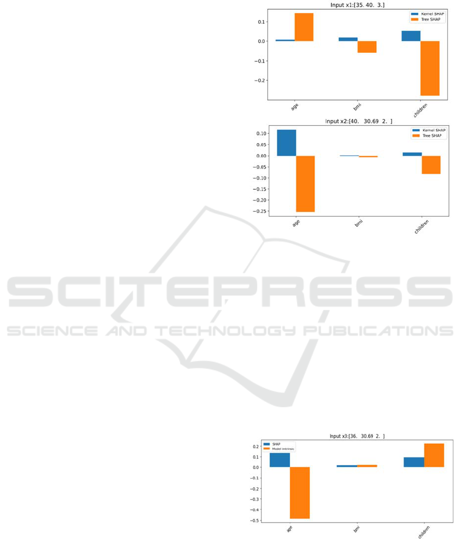
• Feature contribution computed from the two
methods, tree- and kernel-SHAP are compared
for two instances from group northwest [age =
35, BMI = 40, children = 3] and [age = 35, BMI
= 40, children = 2] in Figure 1. It is observed that
these two methods are not aligned in magnitude,
order, and sign.
MLogRM: The model intrinsic feature importance
method of MLogRM is instance-based (local).
Therefore, explanations generated by this method can
be compared to kernel-SHAP explanations per data
instance. To this end, the means of 𝜌

, 𝑃𝑈𝑋, and
𝑃𝑂𝐼𝐹𝑆 over 50 randomly sampled instances from the
training dataset is computed and the process is
repeated 10 times to estimate the KPIs for each
MLM-group. The KPIs for the four MLM-groups are:
•
𝜌

: (0.86  0.07),(0.80  0.05),(0.80  0.09 ),
and
(
0.82  0.06
)
. SHAP feature contribution
ranks are not fully correlated with model intrinsic
ones across the MLM-groups, implying that
SHAP occasionally produces incorrect feature
contribution magnitudes.
Figure 1: Comparison of feature contribution (y-axis) using
tree-SHAP and kernel-SHAP methods for two data
instances in the region northwest.
• 𝑃𝑈𝑋 : (0.1 0.01),(0.09  0.005),(0.07 
0.003), and (0.09  0.01) . There exists
probability gap between model intrinsic and
SHAP of ~
0.1 of an insured being in class 1 for
all MLM-groups. This is moderately significant
in this use-case.
• 𝑃𝑂𝐼𝐹𝑆: (9.2 1.7)%,(3.1  1.04)%,(7.2 
2.06)%, and (2.6  1.36)%. SHAP and model
intrinsic feature contribution signs do not
completely match, implying that there are
instances where SHAP estimates the sign of
feature contributions incorrectly.
Figure 2: Comparison of feature contribution (y-axis) using
kernel-SHAP and Model intrinsic methods for one data
instance in the region northwest.
As demonstrated in Figure 2, kernel-SHAP fails
to accurately detect the sign, magnitude and order of
An Audit Framework for Technical Assessment of Binary Classifiers
321

feature contributions for the given data instance. It is
important to detect such exceptions during audit.
Such examples elucidate that approximate feature
attribution methods such as SHAP can produce
unreliable feature explanations which are not suitable
for many customer facing applications of binary
classifiers.
4.6 Results for Counterfactual
Explanations
For each data point in the test dataset for which the
predicted class is 0, counterfactuals were generated.
The counterfactuals were taken to be the mesh-grid of
values around the data points in the test dataset such
that the range of values for the feature variables are
[𝑥
𝑎𝑔𝑒
− (25+𝑟𝑎𝑛𝑑{0,2}), 𝑥
𝑎𝑔𝑒
+ (25+𝑟𝑎𝑛𝑑{0,2})],
[𝑥
bmi
− (25+𝑟𝑎𝑛𝑑{0,2}), 𝑥
bmi
+ (25+𝑟𝑎𝑛𝑑{0,2})],
[𝑥
child
− (5+𝑟𝑎𝑛𝑑{0,2}), 𝑥
child
+ (5+𝑟𝑎𝑛𝑑{0,2})],
where r𝑎𝑛𝑑{0,2} is a random integer between (0,2).
Note that generating counterfactuals this way is not
optimal, but it is used for demonstration purposes.
RFM: The values computed for PVCF, PCF,
SCF, and DCF are 50.28%, 0.48, 0.04, and 0.52
respectively.
MLogRM: The values computed for PVCF,
PCF, SCF, and DCF are 33.26%, 0.53, 0.04, and 0.47
respectively.
For both RFM and MLogRM, the four KPIs,
PVCF, PCF, SCF, and DCF have a Red RAG score,
implying, the quality of the counterfactuals generated
by the method described above is not adequate and
requires improvements.
5 CONCLUSIONS
In this paper an audit framework for technical
assessment of binary classifiers is proposed along
with KPIs and corresponding RAG scores. The
framework is based on three aspects: model,
discrimination, transparency & explainability. The
framework is demonstrated through its computed
KPIs using an open-source dataset and building two
commonly used binary classifiers, random forests and
multilevel logistic regression. The framework suits
generalized linear models more than tree-based ones.
In the absence of a model intrinsic method to generate
feature importance, no one feature attribution
explainability method, such as SHAP is sufficient.
Also, multiple KPIs are required to assess each
aspect, e.g., if the KPI for Proximity of
counterfactuals declines, the KPI for Diversity
increases. Another example is the discrepancy in the
KPIs for group fairness, Disparate Impact and Equal
Odds.
Future work includes extending the framework to
other classification models and launching pilots in
industry. The latter is expected to provide insights,
which are essential to extend the current scope of the
audit framework beyond technical aspects to include
organizational and process related aspects. Also, it is
worthwhile investigating how an ensemble of
different explainability methods can generate
trustable explanations for model auditability.
REFERENCES
Adedokun, S. T., Uthman, O. A., Adekanmbi, V. T., &
Wiysonge, C. S. (2017). Incomplete childhood
immunization in Nigeria: a multilevel analysis of
individual and contextual factors. BMC public health,
17(1), 1-10.
Angwin, J., Larson, J., Mattu S., & Kirchner, L. (2016).
Machine Bias. Retrieved August 24, 2022 from
https://www.propublica.org/article/machine-bias-risk-
assessments-in-criminal-sentencing
Baldwin, R., Cave, M., & Lodge, M. (2011).
Understanding regulation: theory, strategy, and
practice. Oxford university press.
Beğenilmiş, E., & Uskudarli, S. (2018, June). Organized
behavior classification of tweet sets using supervised
learning methods. In Proceedings of the 8th
International Conference on Web Intelligence, Mining
and Semantics (pp. 1-9).
Bhaumik, D., Dey, D., & Kayal, S. (2022, November). A
Framework for Auditing Multilevel Models using
Explainability Methods. In ECIAIR 2022 4th European
Conference on the Impact of Artificial Intelligence and
Robotics (p. 12). Academic Conferences and
publishing limited.
Biran, O., & Cotton, C. (2017, August). Explanation and
justification in machine learning: A survey. In IJCAI-
17 workshop on explainable AI (XAI) (Vol. 8, No. 1, pp.
8-13).
Breiman, L. (2001). Random forests. Machine learning,
45(1), 5-32.
Chen, V., Li, J., Kim, J. S., Plumb, G., & Talwalkar, A.
(2022). Interpretable machine learning: Moving from
mythos to diagnostics. Queue, 19(6), 28-56.
Commissie, E. (2021). Proposal for a Regulation of the
European Parliament and of the Council laying down
harmonised rules on Artificial Intelligence (Artificial
Intelligence Act) and amending certain Union
legislative acts. Retrieved 01.06.2022: https://eur-
lex.europa.eu/legal-content/EN/TXT/?uri=
CELEX%3A52021PC0206.
Daghistani, T., & Alshammari, R. (2020). Comparison of
statistical logistic regression and random forest
machine learning techniques in predicting diabetes.
ICAART 2023 - 15th International Conference on Agents and Artificial Intelligence
322

Journal of Advances in Information Technology Vol,
11(2), 78-83.
Dumitrescu, E., Hué, S., Hurlin, C., & Tokpavi, S. (2022).
Machine learning for credit scoring: Improving logistic
regression with non-linear decision-tree effects.
European Journal of Operational Research, 297(3),
1178-1192.
Dwivedi, R., Dave, D., Naik, H., Singhal, S., Rana, O.,
Patel, P., ... & Ranjan, R. (2022). Explainable AI (XAI):
core ideas, techniques and solutions. ACM Computing
Surveys (CSUR).
EBA. (2020). Report on big data and advanced analytics.
European Banking Authority.
Esteva, A., Kuprel, B., Novoa, R. A., Ko, J., Swetter, S. M.,
Blau, H. M., & Thrun, S. (2017). Dermatologist-level
classification of skin cancer with deep neural networks.
Nature, 542(7639), 115-118.
Gelman, A., & Hill, J. (2006). Data analysis using
regression and multilevel/hierarchical models.
Cambridge university press.
Ghosh, A., & Maiti, R. (2021). Soil erosion susceptibility
assessment using logistic regression, decision tree and
random forest: study on the Mayurakshi river basin of
Eastern India. Environmental Earth Sciences, 80(8), 1-
16..
Giannakis, E., & Bruggeman, A. (2018). Exploring the
labour productivity of agricultural systems across
European regions: A multilevel approach. Land use
policy, 77, 94-106.
Gunning, D., Stefik, M., Choi, J., Miller, T., Stumpf, S., &
Yang, G. Z. (2019). XAI—Explainable artificial
intelligence. Science robotics, 4(37), eaay7120.
Gupta, G. P., & Kulariya, M. (2016). A framework for fast
and efficient cyber security network intrusion detection
using apache spark. Procedia Computer Science, 93,
824-831.
Hardt, M., Price, E., & Srebro, N. (2016). Equality of
opportunity in supervised learning. Advances in neural
information processing systems, 29.
Kaggle. (2018). US Health Insurance Dataset. [Online].
Retrieved 01.03.2022: https://www.kaggle.com/
datasets/teertha/ushealthinsurancedataset
Kazim, E., Denny, D. M. T., & Koshiyama, A. (2021). AI
auditing and impact assessment: according to the UK
information commissioner’s office. AI and Ethics, 1(3),
301-310.
Kim, H., Cho, H., & Ryu, D. (2020). Corporate default
predictions using machine learning: Literature review.
Sustainability, 12(16), 6325.
Kordzadeh, N., & Ghasemaghaei, M. (2022). Algorithmic
bias: review, synthesis, and future research directions.
European Journal of Information Systems, 31(3), 388-
409.
Loh, H. W., Ooi, C. P., Seoni, S., Barua, P. D., Molinari, F.,
& Acharya, U. R. (2022). Application of Explainable
Artificial Intelligence for Healthcare: A Systematic
Review of the Last Decade (2011–2022). Computer
Methods and Programs in Biomedicine, 107161.
Loyal, J. D., Zhu, R., Cui, Y., & Zhang, X. (2022).
Dimension Reduction Forests: Local Variable
Importance using Structured Random Forests. Journal
of Computational and Graphical Statistics, 1-10..
Lundberg, S. M., & Lee, S. I. (2017). A unified approach to
interpreting model predictions. Advances in neural
information processing systems, 30.
Ma, C., Baker, A. C., & Smith, T. E. (2021). How income
inequality influenced personal decisions on disaster
preparedness: A multilevel analysis of homeowners
insurance among Hurricane Maria victims in Puerto
Rico. International Journal of Disaster Risk Reduction,
53, 101953.
Mehrabi, N., Morstatter, F., Saxena, N., Lerman, K., &
Galstyan, A. (2021). A survey on bias and fairness in
machine learning. ACM Computing Surveys (CSUR),
54(6), 1-35.
Mikians, J., Gyarmati, L., Erramilli, V., & Laoutaris, N.
(2012, October). Detecting price and search
discrimination on the internet. In Proceedings of the
11th ACM workshop on hot topics in networks
(pp. 79-84).
Milanović, S., Marković, N., Pamučar, D., Gigović, L.,
Kostić, P., & Milanović, S. D. (2020). Forest fire
probability mapping in eastern Serbia: Logistic
regression versus random forest method. Forests,
12(1), 5.
Miller, T. (2019). Explanation in artificial intelligence:
Insights from the social sciences. Artificial intelligence,
267, 1-38.
Mohseni, S., Zarei, N., & Ragan, E. D. (2021). A
multidisciplinary survey and framework for design and
evaluation of explainable AI systems. ACM
Transactions on Interactive Intelligent Systems (TiiS),
11(3-4), 1-45.
Molnar, C. (2020). Interpretable machine learning. Lulu.
com.
Mothilal, R. K., Sharma, A., & Tan, C. (2020, January).
Explaining machine learning classifiers through diverse
counterfactual explanations. In Proceedings of the 2020
conference on fairness, accountability, and
transparency (pp. 607-617).
Nawrotzki, R. J., & Bakhtsiyarava, M. (2017). International
climate migration: Evidence for the climate inhibitor
mechanism and the agricultural pathway. Population,
space and place, 23(4), e2033.
Pessach, D., & Shmueli, E. (2022). A Review on Fairness
in Machine Learning. ACM Computing Surveys
(CSUR), 55(3), 1-44.
Rai, N. (2022). Why ethical audit matters in artificial
intelligence? AI and Ethics, 2(1), 209-218.
Raji, I. D., & Buolamwini, J. (2019, January). Actionable
auditing: Investigating the impact of publicly naming
biased performance results of commercial ai products.
In Proceedings of the 2019 AAAI/ACM Conference on
AI, Ethics, and Society (pp. 429-435).
Sarker, I. H. (2021). Machine learning: Algorithms, real-
world applications and research directions. SN
Computer Science, 2(3), 1-21.
Schroepfer, M. (2021, March 11). Teaching fairness to
machines. Facebook Technology. https://tech.fb.com/
teaching-fairness-to-machines/
An Audit Framework for Technical Assessment of Binary Classifiers
323

Stephanopoulos, N. O. (2018). Disparate Impact, Unified
Law. Yale LJ, 128, 1566.
Strobl, C., Boulesteix, A. L., Kneib, T., Augustin, T., &
Zeileis, A. (2008). Conditional variable importance for
random forests. BMC bioinformatics, 9(1), 1-11.
Tosin, M., Côrtes, A., & Cunha, A. (2020). A Tutorial on
Sobol’Global Sensitivity Analysis Applied to Biological
Models. Networks in Systems Biology, 93-118.
van der Rest, J. P., Sears, A. M., Kuokkanen, H., & Heidary,
K. (2022). Algorithmic pricing in hospitality and
tourism: call for research on ethics, consumer backlash
and CSR. Journal of Hospitality and Tourism Insights,
(ahead-of-print).
Wang, L., Abdel-Aty, M., Shi, Q., & Park, J. (2015). Real-
time crash prediction for expressway weaving
segments. Transportation Research Part C: Emerging
Technologies, 61, 1-10.
Xu, Y., Liu, X., Cao, X., Huang, C., Liu, E., Qian, S., ... &
Zhang, J. (2021). Artificial intelligence: A powerful
paradigm for scientific research. The Innovation, 2(4),
100179.
ICAART 2023 - 15th International Conference on Agents and Artificial Intelligence
324